Solving the Potential Field Local Minimum Problem Using Internal Agent States
MH Mabrouk and CR McInnes
Department of Mechanical Engineering, University of Strathclyde, Glasgow, G1 1XJ
{mohamed.mabrouk, colin.mcinnes}@strath.ac.uk
Abstract
We propose a new, extended artificial potential field method, which uses dynamic internal agent states. The internal states are modeled as a dynamical system of coupled first order differential equations that manipulate the potential field in which the agent
is situated. The internal state dynamics are forced by the interaction of the agent with the external environment. Local equilibria in the potential field are then manipulated by the internal states and transformed from stable equilibria to unstable equilibria, allowing escape from local minima in the potential field. This new methodology successfully solves reactive path planning problems, such as a complex maze with multiple local minima, which cannot be solved using conventional static potential fields.
1 Introduction
principles of natural swarms has proven to be a useful tool for the intelligent design and control of artificial robotic agents [3,4].
Swarming robotic systems are often modelled as a two-dimensional collection of point agents in which members may interact with one another through attractive-repulsive pair-wise interactions. Specific choices of potential field can lead agents to self-organize into coherent patterns [5,6]. Recently, swarm stabilization or collapse with increasing constituent number has been predicted along with complex behaviour such as phase transitions and emergent patterns [7,8]. Virtual leaders [9] and structural potential functions [10] have also been introduced to provide provable group behaviour to ensure agents can avoid obstacles and form desired patterns. The actual realization of self-propelled agents interacting according to virtual potentials has also been investigated [11].
These prior studies assume that the free parameters, which define the potential field, are fixed. However, in [12] these parameters were assumed to be internal states for each agent, through which the agent can manipulate the potential field in which it is situated. The dynamics of these internal states are defined through sets of coupled first order differential equations. Then, as an escape path is found, those agents with the greatest speed acquire a stronger attractive potential, thus forming temporary leaders to displace the remainder of the swarm from the local minimum. Here, the internal state concept is extended and applied to problems with multiple local minima. In particular, goal-seeking behaviour in a maze is used to demonstrate that internal states can be used effectively to escape from local minima. As a swarm of agents becomes trapped in a local minimum, the repulsive interaction between agents grows, forcing the agents from the local minimum. We substitute the temporary leader concept with another concept that is found in real biological systems, which is the concept of aggregation of the swarm’s individuals to face a problem [13]. As the agents escape, damping terms in the internal state dynamics then allows relaxation of the potential field.
the agents translate to the goal along the gradient of the potential field. However, in order to prevent collision with a static obstacle, an additional repulsive potential field is required. These two potential fields are then superimposed to form a global potential field, which describes the workspace of the problem. In general however, a local minimum may form due to the superposition of the goal potential and that of the obstacles, resulting in the agent, or swarm of agents, becoming trapped in a state other than the goal G.
1.2 The Local Minimum Problem
The local minima problem has been a serious issue for potential field methods. Early attempts were made to overcome this problem in a variety of ways [14 – 16], none of which provides as a truly efficient solution, and then several attempts have been made
ever since. These attempts can be categorized into two approaches: local minima avoidance (LMA) and local minima escape (LME).
In LMA, local minima are produced in the workspace only at the goal position by modifying the potential field. Navigation functions, harmonic functions, and solenoidal field methods are good examples of such an approach. The navigation function method does not pose local minima, however significant calculations are required [17]. Therefore, this approach may not be practical for real-time motion planning in dynamic or partially known environments. In the harmonic function method, Laplace’s equation is applied to the path planning problem [18]. Although the resulting potential field again does not have local minima, off-line computation is required to provide a solution to the Laplace equation. The solenoidal field method [19] replaces repulsive forces by magnetic-type forces that lead the agent to a path along which it can follow the obstacle boundaries.
In the multi-potential field method, different resolution potential maps are produced. If a local minimum is visible in one potential field map, it can be invisible in another potential map with different resolution. The main drawback of the method is that the agent can come back again to a previously visited local minimum configuration after several circular moves [20]. The random walk method probabilistically enables the agent to escape the local minima region. However, the less informed the potential in use, the larger the random walks in the final path, which is considered the main drawback to the approach [21]. The Straight Line Select (SLS) method, which is a combination of random walks and a straight-line method, finds a new direction for a robot that meets a local minimum by drawing a straight line randomly. If the end point of the line has a lower potential than the local minimum position the agent selects that direction to move. Although combining it with random walks increases the method’s success rate, this
approach is considered unsuitable for real-time motion planning [21]. In the virtual obstacle method [22] when the agent faces a concave shaped obstacle, a virtual obstacle is added and a virtual polygon is made inside the concavity, filling it up. This makes the agent to move toward a calculated point out of the polygon. The main drawback of the method is the heuristic selection of the polygons line lengths, which consequently causes the performance to fall if a poor choice of polygon length has been made.
Another recent example of LME is forward chaining, which is a technique whose target is to provide smooth adaptation of the robot’s path while maintaining persistence towards a goal using intermediate sub-goal attractors. These sub-goals dynamically reshape the potential field to form temporary stepping-stones connecting to the goal, and then other attempts emerge from this technique [23 – 26]. The main drawback is when dealing with deep concave obstacles, where a considerable number of sub goals are to be assigned producing a relatively expensive way of solving the problem.
1.3 Swarm Model
a swarm for simplicity. The swarm model is an extension of that of [7] and consists of Np agents with mass mi, position ri and relative distance rijbetween the ith and jth agents. The agents interact by means of a cohesive two-body generalized Morse potential Vcohesion(ri) with weak long range attraction and strong short range repulsion. For simplicity, we will consider agents of unit mass. To provide dissipation, and so convergence to a static goal, a dissipative term with a positive nonzero coefficient β is added [7]. The total potential field, which affects the ith agent, is then characterized by other agent’s attractive and repulsive potential fields of strength Ca and Cr with ranges la and lr respectively along with obstacle and goal potentials of strength Cio and Cig with ranges lio and lig respectively. In general, the equations of motion for Np agents moving in a workspace that contains No obstacle points at locations rio and Ng goal points at locations rig are then defined by: i i dt d v r = (1)
( )
i total i i i i V dt dm v =−βv −∇ r (2)
( )
i cohesion( )
i goal( )
ig obstacles( )
iototal V V V
V r = r + r + r (3)
Using the generalized Morse potential to define Vcohesion(ri), the cohesion potential among the swarm individuals, Vgoal(rig) the attraction potential of the Ng goals and Vobstacles(rio), the repulsive potential of the No obstacles, will be defined as:
( )
∑
≠ − − − − − = p j a j i j j r j i j N i j l a l r icohesion C e C e
V r r r r r (4)
( )
∑
= − − − = g k ig k g i k N k l ig iggoal C e
V
1
r r
( )
∑
= − − = o n io n o i n N n l io ioobstacles C e
V
1
r r
r (6)
From Eq. (4-6), Eq. (3) will be defined as:
( )
∑
∑
∑
= − − = − − ≠ − − − − + − − = o n io n o i n g k ig k g i k p j a j i j j r j i j N n l io N k l ig N i j l a l r i total e C e C e C e C V 1 1 r r r r r r r r r (7)For a complex potential field such as that represented by Eq. (7), the potential can posses multiple local minima. A key issue is to identify how the agent will realize that it is trapped in a local minimum so that it can then attempt escape. In this case, the agent must be endowed with higher level perception concerning its environment to realize that it is trapped (located in proximity to a local minimum). Then, in order to escape it must learn to discount its immediate sensory information (attraction of the goal), and take action to solve the problem (in our method, manipulate the potential field).
Learning algorithms that incorporate some behaviour from animal development are numerous. For example, Q-learning which is a popular technique for solving a broad class of tasks known as reinforcement learning problems. Using this algorithm, the agent's goal is to modify its own behavior so as to maximize some measure of reward that it receives over time. Q-learning is a powerful algorithm, however it suffers a number of drawbacks among which are that state and action spaces can grow very large such that the processing time and memory requirements for the algorithm are increased [27]. In this
2. Agent Internal States
Escape from complex workspaces can be seen in many natural systems in which the system consists of a number of agents enclosed in a trap. A simple physical example is an ensemble of gas molecules which are enclosed in a single-exit container, while the molecules experience a change in their state due to a rise in temperature for example. The change of the internal state of the system simply changes the trap region from a local minimum into a region of maximum potential from which all the agents are emitted as if squeezed out. The repulsive interaction potential of each agent increases, leading both to an increase in repulsion between agents and between the walls of the trap and so leads to escape [12].
The use of agent internal states will now be considered as a means of allowing agents to manipulate the potential field in which they are manoeuvring. This concept will
be applied firstly to a swarm of agents manoeuvring towards a goal in a potential field which contains a single local minimum, and later to a swarm negotiating a maze with multiple local minima. The agents’ internal states will now be defined through a set of first order differential equations which will allow the swarm of agents to manipulate the potential field in which they are manoeuvring and so escape from a local minimum. For a fixed set of obstacles, the repulsion potential range affecting the ith agent lio can be represented as a function of an obstacle constant lo, which characterizes the physical size of the obstacle, and the agent repulsion potential range lri which characterizes the agent internal state. The obstacle repulsion potential strength affecting the ith agent Cio will be represented as the obstacle constant Co. The attraction potential range of the goal affecting the ith agent lig will be represented as a function of a goal constant lg, which characterizes the physical nature of the goal. The attraction potential strength of the goal affecting the ith agent Cig will be represented as the goal constant Cg such that:
o
io C
C = (8)
ri o
io l l
l = + (9)
g
ig C
g
ig l
l = (11)
When an agent approaches an obstacle, as shown in Fig. 1, it will experience repulsion that displaces the agent away from the goal. However, the superimposed attraction of the goal can then lead to the formation of a local minimum in the potential field. The agent
will never attempt to manoeuvre around the fixed obstacle simply because it never knows that it is trapped. Both the global and local minima of the potential field satisfy the
equilibrium state ∇iVtotal
( )
ri =0 from Eq. (2). In addition, the speed of the centre-of-mass of a cohesive swarm will increase as the swarm approaches the goal and decreases as it is repelled by an obstacle, while the swarm is trapped if it enters a local minimum of the potential field. The speed of the centre-of-mass of the swarm will now be used as an effective mechanism for the swarm to increase its perception about its progress through the workspace, and so avoid trapping in local minima. The swarm individuals should be guaranteed to maintain a cohesive group for two reasons (1) to magnify the effect of the speed of the centre-of-mass of the swarm on the global perception of the swarm, (2) to ensure the swarm aggregates to face the problem collectively as noted in studies of real biological systems [13].We now introduce a function Qc, inspired from learning by reward or punishment in real biological systems [28,29]. The function is defined by the change of the modulus
of the speed of the centre-of-mass of the swarm measured over some finite time interval. If the swarm is being repelled away from the goal Qc will have a negative value, which is viewed as punishment, indicating that a part of or the entire swarm is moving away from the goal. If Qc ≥ 0, which is the viewed as reward, the swarm senses collectively that it is moving towards the goal.
We now allow the free parameters of the potential field to be dynamic internal states and couple these internal states of the agent’s perception of its progress through the workspace. If the agent is progressing towards the goal, or the position of the
The following set of first order differential equations are now posed to express the internal states of the ith agent:
≤ − ≥ < − = − ε λ λ | Q Q C e A dt dC g c c c ri r Q r
ri q c
r r | or 0 0
0 (12)
≤ − ≥ < − = − ε λ λ | Q Q l e B dt dl g c c c ri r Q r
ri q c
r r | or 0 0
0 (13)
≤ − ≥ < − = ε λ λ | | or 0 0 0 | | g c c c ai a a ai Q Q C e A dt
dC v i
r r v (14) ≤ − ≥ < − = ε λ λ | | or 0 0 0 | | g c c c ai a a ai Q Q l e B dt
dl v i
r r v (15)
(
)
≥ < − − + = 0 0 0 1 c c i i i Q Q | | exp A dtdβ β λββ
v (16)
Equations (12-15) express the repulsion amplitude and range and the attraction amplitude and range of the ithagent, according to the speed of each agent as well as the value of the function Qc which depends on the speed of the centre-of-mass of the swarm. When the agents are repelled from an obstacle, the speed of the centre-of-mass of the swarm decreases, lio then increases due to Eq. (9,13) which turns the workspace in the neighborhood of the obstacles into a zone of maximum potential. This then leads to escape from the local minima, while the potential field relaxes after escape due to the damping terms in the differential equations for the internal states.
The cohesion generated by Eq. (14, 15), ensures aggregation amongst the swarm’s individuals to face the local minimum problem and the net effect is then that the trapped swarm is forced to simultaneously explore escape paths. Moreover, Eq. (16) ensures
to its speed. The damping terms in Eq. (12-16) ensure that the deviation of the agent internal state relaxes and returns to an equilibrium value as soon as the local minimum problem is solved. The coefficients Ar, Br, Aa, Ba, Aβ, λq, λr, λv, λa, λβ are employed to
scale the dynamics of the internal states.
3. Analysis of Agent Internal States
3.1 Analysis for Qc ≥ 0
In this section, we will investigate the role of the function Qc to solve the local minimum problem. Using the dynamic internal states defined in Eq. (12-16), the potential field is now a function of five parameters for each agent. According to the equations of motion, Eq. (1, 2), and assuming unit mass, the equation of motion of the ith agent is:
( )
i total i i i V dt d r v r ∇ − − = β 2 2 (17)It will firstly be assumed that agent does not encounter any obstacles so that Qc≥0. From Eq. (7), the generalized Morse potential for an obstacle-free workspace with one goal scenario is defined as:
( )
i g igp j a j i j j r j i j l ig N i j l a l r i
total C e C e C e
V r r r r r −r −r
≠ − − − − − −
=
∑
(18)The effective energy of the swarm will then be defined as follows:
( )
∑
+ = p N i i total i i Vm v 2 r
2 1
φ (19)
(
)
) ( ) ( 2 2 2 ig ig ig ig p j a ij j j j j r ij j j j p j a ij j p j r ij j p l / | | ig ig ig . ig l / | | ig . N i l / | | a ij a . a l / | | r ij r . r N i l / | | a . N i j l / | | r . N i i total i i i i . e l | | l C e C e l | | l C e l | | l C e C e C V m r r r r r r r r r v v v − − − − − ≠ − + − − + − + ∇ + =∑
∑ ∑
∑
φ (20)However, since Qc≥0, substituting from Eq. (8-15), it can be seen that:
∑
− = p N i i i 2 . vβ
φ
(21)Since βi has a positive nonzero value, it can be seen that 0 .
<
φ , and so the swarm will
converge asymptotically to the goal.
3.2 Analysis for Qc < 0
It will now be assumed that that agent does encounter an obstacle so that Qc<0. From Eq. (2-3) it can be seen that:
( )
i i goal( )
ig i obstacles( )
io cohesion i i i i V V V dt d r r r v r ∇ − ∇ − ∇ − − = β 2 2 (22)We note that in general the gradient terms can be replaced with scalar derivatives and unit vectors such that:
( )
io io obstaclesio obstacles
iV (r )=V' r ˆr
∇ (23)
( )
∑
≠ = ∇ p N i j ij ij cohesion i cohesion( )
ig ig goalig goal
iV (r )=V' r ˆr
∇ (25)
where (‘)=∂()/∂ri. Therefore, defining the location of the centre-of-mass of the swarm as
∑
≠ − = p N i j i pc N r
r 1 , Eq. (22), shows that the acceleration of the centre-of-mass of the swarm
will be defined by:
( )
( )
( )
+ + + − =∑
∑
∑
∑
∑
= = ≠ = = io io obstacles N i ig ig goal N i ij ij cohesion N i j N i N i i i p c ˆ ' V ˆ ' V ˆ ' V N d d o p p p p r r r r r r v r 1 1 1 1 2 2 1 t β (26)Since ˆrij =−ˆrji, the internal cohesion forces will cancel over the double summation to yield:
( )
( )
+ + − =∑
∑
∑
= = = io io obstacles N i ig ig goal N i N i i i p c ˆ ' V ˆ ' V N dd p p o
r r r r v r 1 1 1 2 2 1 t β (27)
In order to demonstrate the change in stability properties of the local minimum using the dynamic agent internal states, we now consider a simplified 1-dimensional analysis
where the goal, local minimum and agent are consider to be collinear so that ˆrig =ˆrio. It will be shown that the effect of using function Qc along with the change in internal state of the agents is to convert the potential field local minimum to a local maximum. From Eq. (7), for a single goal and single obstacle, the potential field is then:
( )
i o io ri rg ligig l r r io i
total r C e C e
V = − − − − − (28)
( )
i o io ri rg lig ig ig l r r io io i i total e l C e l C r rV − − − −
+ − = ∂ ∂ (29)
We will assume that rm is the position of a local extremum that forms in the global potential field according to the superposition of the goal and the obstacle potential fields
so that ∂
( )
∂ = =0m i r r i i
total r r
V . Then from Eq. (29), it is then clear that
(
)
(
)
mo l r r mo mo mg l r r mg mg r e l C r e lC − m− g mg − m− o mo
= (30)
which defines the condition for equilibrium at the extremum position rm. From Eq. (29), it can also be seen that
( )
(
)
(
)
+ − ∂ ∂ = ∂∂ − i−o io −ri−rg lig
ig ig l r r io io i i i total e l C e l C r r r V 2 2 (31)
Then, for extremum position rm and substituting from Eq. (30) it can be seen that
( )
(
)
− = ∂ ∂ − −= mo mg
l r r mo mo r r i i total l l e l C r r
V m o mo
m i 1 1 2 2 (32)
We will now consider the behavior of Eq. (32) for different signs of Qc. For a swarm that has a clear path to the goal, Qc≥ 0 and so we conclude that lmo < lmg which, according to
Eq. (32), means that ∂2
( )
∂ 2 >0 = m i r r i itotal r r
V , so that a local minimum forms as
expected. However, for Qc < 0, the internal state dynamics ensure that lmo increases so
that lmo > lmg which, according to Eq. (32), means that ∂2
( )
∂ 2 <0 =m i r r i itotal r r
V and so
states dynamics then ensure that the potential field relaxes after being manipulated by the agent. This behavior will now be demonstrated in simulation.
4. Simulation Results
4.1 Local Minimum Problem Solving
First, the case of a swarm whose agents are using fixed internal states will be considered. Here, the free parameters describing the potential field, and so the potential field itself, are constant. The simulation results in Fig. 2 show a swarm of agents in which part of the swarm becomes trapped in the local minimum of the potential field, which forms behind a C-shape obstacle that is constructed from No obstacle points, while the rest of the swarm reaches the goal according to their initial positions. This situation has the further
disadvantage of increasing the depth of the local minimum, thus increasing the difficultly for the trapped agents to escape. This is typical of conventional implementations of the artificial potential field method to path planning problems.
the goal. The comparison between the results in Fig. 2 and Fig. 3 clearly shows the effect of using the internal state dynamics to solve the problem effectively.
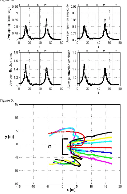
Regions I, II, III, IV and V of Fig. 4 explain the stages of the simulation demonstrated in Fig. 3. First the swarm is moving towards the goal with fixed internal states, as shown in region I. Then, when the lead part of the swarm is repelled, the repulsion potential increases then the velocities of the repelled agents increase and consequently the attraction potential increases amongst agents and they aggregate. After the aggregation process, region II, the potential relaxes and the swarm is attracted to the goal as a coherent flock. Region III in Fig. 4 shows that the interaction parameters remain fixed as Qc > 0 when the flock is moving towards the goal. Region IV of Fig. 4 shows that when the swarm is repelled by the obstacle, the average repulsion potential between the swarm and the obstacle increases (as an effect of using the function Qc). However the repulsion also makes the agent velocities to increase, which increases the inter-agent attraction potential, ensuring that the entire swarm escapes. It should be noted that it is only the increasing agent repulsion which is solving the local minimum problem. The increasing inter-agent attraction merely ensures that the entire swarm remains cohesive and escapes [12]. As soon as the problem is solved a relaxation in the potential takes place and the interaction parameters are fixed again at their final values, as shown in region V of Fig. 4.
We use the internal state model to solve the problem for the swarm of agents starting from different initial positions around the obstacle to show the efficiency and robustness of the model. The path of the swarm’s centre-of-mass for different initial positions is demonstrated in Fig. 5, with the middle starting position representing the path of the swarm in Fig. 3. For the results shown in Fig. 3 and Fig. 5 all control parameters are unity.
4.2 Maze Problem Solving
conventional static potential field. The simulation results, shown in Fig. 6, demonstrate the capability of the swarm using the internal state model to solve the problem and reach the goal, while the other conventional swarm is trapped in the first level of the maze. Fig. 7 shows the path of the centre-of-mass of the swarm through the maze to the goal. The different levels of difficulty for the different parts of the maze require the determination of the control coefficients to cope with the most difficult level. This may cause a relatively higher overshoot in flock behaviour in one of the maze levels. For the maze application in Fig. 7, the control coefficients are all unity except Ar =1.5, Br =1.5, Aβ
=0.7.
Finally, we consider another application of internal states related to crowd dynamics using communication through local interactions between swarm members such that the value of the perception function will be calculated on an individual basis (i.e.
calculating a perception function Qi for each agent based on its behaviour). Here, we use a modified algorithm to ensure that those agents who have a clear path to the goal, emerge as the leaders for the agents trapped in the local minimum of a static potential.
The scenario, shown in Fig. 8, demonstrates a swarm that uses fixed internal states in two groups. The first group has a clear path to the goal while the other group is trapped in a local minimum formed behind a C-shape obstacle. The individuals of the swarm, which are trapped in the local minimum, were clearly not led to the goal by the other agents that successfully reach the goal. We now compare this scenario with part of the swarm using the modified dynamic internal state model, as show in Fig. 9. Group a
We note that although the method is relatively simple computationally, it will have implementation limitations for real-world applications. Clearly, the location of each agent in the group must be known to every other agent in order to update the value of the function Qc for the entire swarm individuals. For agents with only nearest neighbour communication this will be difficult, since global information must then be distributed through the swarm via local communication. However, given the exponential decay of terms in the various potential fields, the algorithm, could be modified to consider only local interactions.
5. Conclusions
This paper presents a new method to escape from the local minima that form during potential field based path planning of robots by using dynamic internal states. Rather than
a static potential field, the agents are able to manipulate the potential field through their internal states according to their estimation of their progress through the workspace. The method allows a swarm of agents to escape from and manoeuvre around a local minimum in the potential field to reach a goal. The method has been demonstrated in problems with a single local minimum and a maze with multiple local minima.
References
[1] P. Maes, Modelling adaptive autonomous agents, Artif. Life1 (1-2) (1994) 135 - 162.
[2] S.Camazine, J. Deneubourg, N. Franks, J. Sneyd, G. Theraulaz, E. Bonabeau, Self organization in biological systems, Princeton University Press, Princeton, NJ, 2003.
[3] E. Bonabeau, M. Dorigo, G.Theraulaz, Swarm intelligence: From natural to artificial systems, Oxford University Press, New York, 1999.
[4] V. Gazi, K. Passino, Stability analysis of swarms, IEEE Transactions in Automatic Control, (48) (2003). 692-697.
[5] H. Levine, W. Rappel, I. Cohen, Self-organization in systems of self-propelled agents, Phys. Rev. E, (63) (2000) 017101.
[6] V. Gazi, K. Passino, A class of attractions/repulsion functions for stable swarm aggregations, in: Proceedings of Conference Decision Control, Las Vegas, NV, USA, (2002) 2842-2847.
[7] M. D’Orsogna, Y.Chuang, A. Bertozzi, L. Chayes, Self-propelled agents with soft-core interactions: Patterns, stability, and collapse. Physical Review Letter (96) (2006) 104302.
(2007) 032904.
[9] Y. Chuang, Y. Huang, M. D’Orsogna, A. Bertozzi, Multi-vehicle flocking: Scalability of cooperative control algorithms using pairwise potential, in: Proceedings of the IEEE International Conference on Robotics and Automation, Roma, Italy, (2007) 2292-2299.
[10] R. Olfati-Saber, Flocking for multi-agent dynamic systems: Algorithms and theory, IEEE Transactions on Automatic Control, Vol. 51, No. 3, (2006) 401-420. [11] B. Nguyen, Y. Chuang, D. Tung, C. Hsieh, Z. Jin, L. Shi, D. Marthaler, A.
Bertozzi, R. Murray, Virtual attractive repulsive potentials for cooperative control of second order dynamic vehicles on the caltech MVWT, in: Proceedings of American Control Conference, Portland, OR,USA, (2005). 1084 -1089.
[12] M. Mabrouk, C. McInnes, Swarm robot social potential fields with internal agent dynamics, in: Proceeding of the Twelfth International Conference on Aerospace Sciences and Aviation Technology (ASAT12), Cairo, Egypt, (ROB-02) (2007)1-14.
[13] M., Lindauer, Communication among social bees, Cambridge, Massachusetts: Harvard University Press 1971.
[14] D. Koditschek, Exact robot navigation by means of potential functions: Some topological consideration, in: proceedings of IEEE Conference on Robotics and Automation, (1987) 1-6.
[15] J. Latombe, Robot motion planning, 101 philip Drive, Assinippi Park, Norwell, MA 02061: Kluwer Academic Publishers, 1991.
[16] N. Franceschini, J. Pichon, C. Blanes, From insect vision to robot vision, Philosophical Transactions of the Royal Society B, (337) (1992) 283-294.
[17] E. Rimon, D. Koditscheck, Exact Robot Navigation Using Artificial Potential Functions. IEEE Transactions on robotics and automation 8 (5) (1992) 501- 518 [18] C. Connolly, J. Burns, R. Weiss, Path planning using laplace's equation, in:
Proceedings of IEEE International Conference on Robotics and Automation 3 (1990) 2102 - 2106
[19] L. Singh, J. Wen, H. Stephanou, Real-time robot motion control with circulatory fields, in: Proceedings of the IEEE International Conference On Robotics and Automation, Minneapolis, Minnesota, (1996) 2737-2742.
[20] H. Chang, A new technique to handle local minimum for imperfect potential field based motion planning, in: Proceedings of the IEEE International Conference on Robotics and Automation Minneapolis, Minnesota, (1996) 108-112.
[21] S.Caselli, M. Reggiani, R. Rocchi, Heuristic methods for randomized path planning in potential fields, in: Proceedings of IEEE International Symposium on Computational intelligence in Robotics and Automation, Banff, Alberta, Canada, (2001) 426- 431.
[22] L. Chengqing, H. Marcelo, H. Krishnan, L. Yong, Virtual obstacle concept for local-minimum-recovery in potential-field based navigation, in: Proceedings of the IEEE International Conference on Robotics & Automation San Fransisco, CA, (2000) 983-988.
[24] J. Lewis, M. Weir, Using sub-goal chaining to address the local minimum problem, in: Proceedings of the International ICSC Symposium on Neural, Computation (2000).
[25] G. Bell, M. Weir, Forward chaining for robot and agent navigation using potential fields, in: Proceedings of Twenty-seventh Australasian Computer Science Conference (ACSC2004), (2004) 265 - 274.
[26] Z. Xi-yong, Z. Jing, Virtual local target method for avoiding local minimum in potential fields based navigation, Journal of Zhejiang University SCIENCE 4 (3) (2003) 264-269.
[27] L. Lin, Reinforcement Learning for robots using neural networks, PhD thesis, Carnegie Mellon University 1993.
[28] N. Mackintosh, Conditioning and associative learning, Oxford: Oxford University Press, 1983.
[29] D. Lieberman, Learning: Behaviour and cognition, Belmont, CA: Wadsworth Publishing Company, 1990.
Figure Captions
Figure 1. Behaviour of an agent with fixed internal states moving to a goal G, (a) t =0 (b)
t =66.
Figure 2. Behaviour of a swarm with fixed internal states. Np =21, No =101, Cg =50, lg =25, Co =4, lo =0.25, (a) t =2 (b) t =73.
Figure 3. Swarm solves a reactive problem using the internal state model. Np =21, No =101, Cg =50, lg =25,Co =4, lo =0.25, (a) t =2 (b) t =12 (c) t =38 (d) t =49 (e) t =56 (f) t =61.
Figure 4. Average interaction parameters of the swarm in Fig. 3, until t =75.
Figure 5. Paths of swarms for different initial positions; middle path is the path of the swarm in Fig. 3.
Figure 6. Maze application for agents using the internal state model; swarm A
symbolized (*), and those with a static potential; swarm B symbolized ( ). Cg =40, lg =15, Co =7, lo =0.1, (a) t =3 (b) t =7 (c) t =9 (d) t =16 (e) t =19 (f) t =25.
Figure 7. Path of swarm A center (with the internal state model) to the goal.
Figure 8. Behaviour of a swarm using fixed internal states. Np =5, Cg =50, lg =25, Co =7,
lo =0.1, (a) t =2 (b) t = 30 (c) t =35 (d) t =70.
Figure 1a.
Figure 1b.
x [m] y [m]
Figure 2a.
Figure 2b.
x [m] y [m]
x [m] y [m]
x [m] y [m]
Figure 3a.
[image:23.612.95.481.86.684.2]x [m] y [m]
y [m]
x [m] Figure 3c.
[image:24.612.93.482.92.709.2]x [m] y [m]
y [m]
x [m] Figure 3e.
[image:25.612.95.480.83.693.2]x [m] y [m]
y [m]
x [m] Figure 3g.
[image:26.612.95.481.84.690.2]x [m] y [m]
x [m] y [m]
[image:27.612.89.481.73.693.2]I II III IV V
I II III IV V
I II III IV V
I II III IV V
[image:28.612.90.498.75.700.2]x [m] y [m]
Figure 4.
Figure 6b.
x [m] y [m]
x [m] y [m]
[image:29.612.92.481.79.699.2]x [m] y [m]
Figure 6c.
Figure 6d.
[image:30.612.95.481.88.697.2]Figure 6e.
Figure 6f.
x [m] y [m]
Figure 6g.
Figure 6h.
x [m] y [m]
Figure 7.
y [m]
x [m] Figure 8a.
x [m] y [m]
x [m] y [m]
Figure 8b.
[image:34.612.88.482.78.689.2]y [m]
x [m]
x [m] y [m]
Figure 8d.
[image:35.612.88.483.78.690.2]x [m] y [m]
x [m] y [m]
Figure 9b.
[image:36.612.88.482.78.694.2]y [m]
y [m]
x [m] Figure 9d.
Figure 9e.
[image:37.612.88.483.79.693.2]
x [m] y [m]
[image:38.612.94.484.78.372.2]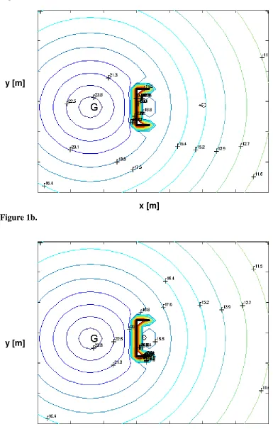
![Figure 2a. y [m]](https://thumb-us.123doks.com/thumbv2/123dok_us/1710630.124462/22.612.95.481.97.689/figure-a-y-m.webp)
![Figure 3a.y [m]](https://thumb-us.123doks.com/thumbv2/123dok_us/1710630.124462/23.612.95.481.86.684/figure-a-y-m.webp)
![Figure 3c.y [m]](https://thumb-us.123doks.com/thumbv2/123dok_us/1710630.124462/24.612.93.482.92.709/figure-c-y-m.webp)
![Figure 3e.y [m]](https://thumb-us.123doks.com/thumbv2/123dok_us/1710630.124462/25.612.95.480.83.693/figure-e-y-m.webp)
![Figure 3g.y [m]](https://thumb-us.123doks.com/thumbv2/123dok_us/1710630.124462/26.612.95.481.84.690/figure-g-y-m.webp)
![Figure 3i.y [m]](https://thumb-us.123doks.com/thumbv2/123dok_us/1710630.124462/27.612.89.481.73.693/figure-i-y-m.webp)
![Figure 6a.y [m]](https://thumb-us.123doks.com/thumbv2/123dok_us/1710630.124462/29.612.92.481.79.699/figure-a-y-m.webp)
![Figure 6d.y [m]](https://thumb-us.123doks.com/thumbv2/123dok_us/1710630.124462/30.612.95.481.88.697/figure-d-y-m.webp)
