Robust multi-objective optimisation of a descent guidance strategy for a TSTO spaceplane

ROBUST MULTI-OBJECTIVE OPTIMISATION OF A DESCENT

GUIDANCE STRATEGY FOR A TSTO SPACEPLANE

Lorenzo A. Ricciardi

_{, Christie Alisa Maddock}

_{, Massimiliano Vasile}

_{, Tristan Stindt}

_{, Jim Merrifield}

Marco Fossati

_{, Michael West}

_{, Konstantinos Kontis}

_{, Bernard Farkin}

_{, Stuart McIntyre}

a

_{University of Strathclyde, Glasgow, UK}

_{Fluid Gravity Engineering, Emsworth, UK}

c

_{BAE Systems, Prestwick, UK}

_{University of Glasgow, Glasgow, UK}

e

_{Orbital Access, Prestwick, UK}

ABSTRACT

This paper presents a novel method for multi-objective op-timisation under uncertainty developed to study a range of mission trade-offs, and the impact of uncertainties on the evaluation of launch system mission designs. A memetic multi-objective optimisation algorithm, MODHOC, which combines the Direct Finite Elements transcription method with Multi Agent Collaborative Search, is extended to ac-count for model uncertainties. An Unscented Transformation is used to capture the first two statistical moments of the quantities of interest. A quantification model of the uncer-tainty was developed for the atmospheric model parameters. An optimisation under uncertainty was run for the design of descent trajectories for the Orbital-500R, a commercial semi-reusable, two-stage launch system under development by Orbital Access Ltd.

Index Terms— Spaceplane, Optimisation under Uncer-tainty,

1. INTRODUCTION

This paper presents a novel method for multi-objective op-timisation under uncertainty, developed to study a range of mission trade-offs and the impact of uncertainties on system models for launch systems. This is applied to the analysis and design of descent trajectories for the Orbital-500R, a commer-cial semi-reusable, two-stage launch system under develop-ment by Orbital Access.

The set of Pareto-optimal solutions show the trade-off be-tween minimising the induced acceleration limits and max-imising the robustness of the solutions by minmax-imising the sen-sitivity to uncertainties.

Uncertainty quantification (UQ), the science of quantify-ing the uncertainty in the desired performance of a system, can be a key step in analysing the robustness of a control solu-tion and of the whole guidance, navigasolu-tion and control (GNC)

chain. Common approaches to UQ use extensive Monte Carlo simulations to account for errors, unmodelled components and disturbances. At system level, UQ analysis can trans-late into the assessment of the whole system reliability or the reliability of one or more components. An uncertainty quan-tification analysis is, therefore, a fundamental step towards de-risking any technological solution as it provides a quan-tification of the variation in performance and probability of recoverable or unrecoverable system failures, given existing information.

Within the current preliminary design phase of the Orbital-500R, one of the areas of study is the uncertainty related to the aerodynamic modelling of the re-usable spaceplane.

The goal is, therefore, to design a robust guidance tra-jectory considering the uncertainty related to the atmospheric model which in turn affects the aero-, aerothermal and flight dynamics. Furthermore, given the early stage of the vehicle design and the wide scope of use required by the commer-cial side, a number of re-entry scenarios are possible, each of which is affected differently by the same sets of uncertainties. This paper presents an extension of the capabilities of MODHOC to account for uncertainties. The extension is based on an Unscented Transformation to capture the first two statistical moments of the quantities of interest. The result is an unscented multi-objective optimal control ap-proach that can efficiently handle the level of uncertainty in model parameters. Using multiple objective functions, trade-off studies on the Orbital-500R design will be presented for the chosen performance and vehicle characteristics of the re-entry trajectory and the robustness of those performances (and the associated guidance laws) against the uncertainty of the atmospheric model.

2. OPTIMAL CONTROL

(DFET), a transcription method for nonlinear multi-phase optimal control problems [3], with MACS, a population based memetic multi-objective optimisation algorithm [4] and mathematical programming solvers. The DFET transcription method allows to treat general optimal control problems, thus it can tackle problems with any kind of dynamic model. The memetic multi-objective optimisation algorithm MACS allows for a global exploration of the search space and is able to treat problems with an arbitrary number of objectives. The mathematical programming solvers are used to refine the solutions obtained and guarantee the local optimality of the solutions found while also satisfying tight constraints.

The software has been successfully used for the trajec-tory and design optimisation of vertical and horizontal launch systems [5, 6], deployment of constellations [7], interplane-tary exploration missions [8] and the design of multi-debris removal missions.

2.1. Unscented optimal control

In order to perform robust optimisation of the re-entry trajec-tory of the Orbital 500R, an Unscented Transformation [9] was included in the formulation of the optimal control prob-lem.

Unscented Transformations capture the first statistical moments, mean and covariance, of the distributions of the states of a system subject to uncertainty and undergoing ar-bitrary non-linear transformations by propagating a small number of sigma points. If the system depends onNuq

un-certain variables, whose mean and covariances are known, the unscented transformation requires the propagation of 2Nuq+ 1samples. The first sigma point takes the mean value

for all the uncertain variables, while the others assume the mean plus (or minus) the square root of the matrix of the covariances of the uncertain variables. All the sigma points are propagated simultaneously with the mean and covariance of the final states computed as a weighted combination of the final states of each sigma point.

The approach employed in this paper follows the one de-scribed by [10]. Let the dynamics of the systems be given by

˙

x=F(x,u,buq, t) (1)

wherex are the states of the system, uare the controls, t is time, and buq are additional static parameters which are

here assumed to be affected by uncertainty. The dynamics of each sigma pointχi, i = 1. . . ,2Nuq+ 1is given byχ˙i =

F(χi,u,bi, t).

This means that each sigma point has a different value for the static variables, its dynamics evolve independently of the other sigma points, but all sigma points are controlled by the same control law. The idea is thus to find a single control law that, when applied to all sigma points, allows the ensemble to reach a desired final condition and to be optimal in some

sense. The particular values for each static variablebiis

de-cided by the application of the Unscented Transformation. A known problem of the Unscented Transformation is that it can generate covariance matrices that are not semidefinite positive. To avoid this problem, a more recent and stable ver-sion of the Uncertain Transformation was employed in this paper, called the Square Root Unscented Transformation [11]. Algorithmically it is very similar to the standard version, but it differs in the way the samples are generated and has the ad-vantage that the resulting covariance matrix is guaranteed to be semidefinite positive (up to machine precision). In prac-tice, the sigma points are thus computed from the Cholesky factorisation of the covariance matrix, and slightly different algebraic manipulations are performed to obtain the covari-ance matrix of the transformed states.

Mathematically, thus, the problem can be described as fol-lows: letXbe a state vector of lengthNσNx,

X:=

χ0_,χ1_{,· · ·,χ}NσT

(2)

whereNσis the number of sigma points andNxis the number

of states of the original system. The dynamics of this system is then given by

˙ X:=     

f(χ0,u,b0, t)

f(χ1,u,b1, t)

.. . f(χNσ_,u,b

Nσ, t)



   

:=F(X,u,B, t) (3)

The multi-objective unscented optimal control problem can thus be formulated as

min

u∈UJ(X,u,B, t)

s.t. ˙

X=F(X,u,B, t) g(X,u,B, t,≥0

ψ(X(t0),X(tf),u(t0),u(tf),B, t0, tf)≥0

t∈[t0, tf]

(4)

In this work, since there is no uncertainty about the ini-tial state of the system, the iniini-tial conditions are expressed as usual. The final conditions, instead, are expressed as differ-ence between the mean and the target value.

ψ(X(tf)) :=µχ−x(tf) = 0 (5)

whereµ_χ is the mean of the final states of the sigma points, andx(tf)is the target value. The first objective

J1:=

Z tf

t0

E(a2)dt (6)

The second objective is meant to reduce the uncertainty of the final state. To this end, the sum of the square of all the en-tries of the covariance matrix of the final states is minimised.

J2=

X

i,j

(Covi,j(X(tf))2 (7)

whereCovi,j is computed using the standard algebraic

ma-nipulations employed for the Square Root Unscented trans-formation, with the additional consideration that no update of the Cholesky factorisation is needed since no measurement is here performed and thus no error is present. This formula-tion has the advantage that the quantity to compute is smooth and differentiable, it involves all components of the covari-ance matrix, and does not require iterative procedures like de-composition in eigenvalues to compute the principal axes of the ellipsoid of the uncertainty. In order to give each element of the covariance matrix the same weight even if the quanti-ties of interest have different scales, the state variables were scaled by the same factors internally employed by MODHOC to ensure that all variables assume values between 0 and 1.

3. VEHICLE SYSTEM MODELS

The Orbital-500R system is composed of a first stage reusable spaceplane, capable of rocket-powered ascent and an unpow-ered, glided descent, and an expendable, rocket-based upper stage. The dry mass of the spaceplane is 20 tonnes.

The flight dynamics are modelled as a variable-mass point with three degrees of freedom in the centered Earth-fixed reference frame, subject to gravitational, aerodynamic lift and drag forces. The state vector contains the transla-tional position and velocity, and time-dependant vehicle mass, x = [h, λ, θ, v, γ, χ, m]wherehis the altitude, (λ, θ)are the geodetic latitude and longitude,vis the magnitude of the relative velocity vector directed by the flight path angleγand the flight heading angle χ [12]. The vehicle is controlled through the angle of attackα, and the bank angle µof the vehicle. The Earth is modelled as a perfect sphere of radius RE.

The aerodynamic coefficients were modelled using an ar-tificial neural network with given an aerodynamic database for the training data coming from CFD simulations [13].

From previous work on the optimisation of the full ascent and reentry trajectory, the vehicle is assumed to begin its re-entry (at timet= 0) with the following initial conditions:

Altitudeh(0) = 90 km

Latitudeλ(0) = 60◦N

Longitudeθ(0) =−12◦E

Velocityv(0) = 3km/s

Flight path angleγ(0) =−5◦

Heading angleχ(0) = 20◦

The only final condition imposed was the expected value of the altitude, with a value of 10 km. In addition, the trajec-tories of all sigma points were required to have a flight path angle greater or equal to−20◦.

4. UNCERTAINTY QUANTIFICATION

Analysis to date on the design of the Orbital 500-R has em-ployed the 76 Standard atmospheric model [14]. The US-76 is a global static standard model, giving the atmospheric pressurep, temperatureT and densityρas function of alti-tude up to 1000 km.

In order to assess the robustness of the design against un-certainties in the atmospheric model, it was necessary to de-velop a model for its uncertainty. To this end the NRLMSISE-00 [15] atmospheric model was employed. It is more recent and sophisticated than the US76 model, and takes into ac-count several factors like daily and seasonal effects, solar and magnetic activity and geographical dependencies. This model thus gives temperature and density as a function of 7 other in-put parameters in addition to altitude.

A statistical analysis of the difference of the models was performed treating those 7 additional input parameters as un-certain.100000samples were taken from the low discrepancy Halton sequence, and the corresponding values forT andρ were computed using the NRLMSISE-00 model for all alti-tudes in the range between 0 and 100 km.

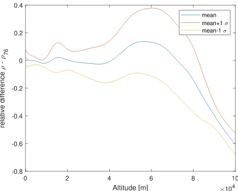
To account for the possible differences between the mod-els, the relative average difference between the values of the two model was computed for all the thermodynamic quanti-ties. These relative errors were then treated as random fluctu-ations, for which averages and covariances were computed as a function of altitude. These relative errors and covariances deviations are plotted in Figures 1, 2 and 3.

Fig. 2. Relative error between models, pressure

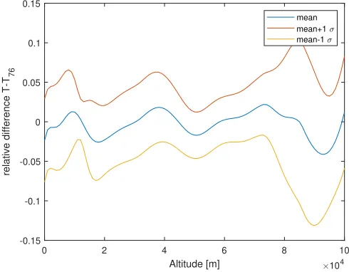
Fig. 3. Relative error between models, temperature

It can be observed that for the temperature the mean rel-ative errors are very low, with a1σrelative error around 5% for altitudes below 80 km. The mean relative errors for pres-sure and density are also low for relatively low altitudes, but they tend to drift systematically at higher altitudes, and the1σ bands are much wider. This happens above 40km where pres-sure and density have a very low absolute value, so a large relative error still means a low absolute error. It is thus ex-pected that the impact of these relatively high differences in density between the two models will not affect significantly the first part of the trajectory.

Since the approach employed is that of the Square Root Unscented Transformation, different models were generated: one employing the mean relative error, and the others adding to the mean the Cholesky factorisation of the covariance

ma-trix of the uncertain quantities at each altitude. Figure 4 shows the five generated temperature profiles, and their comparison with respect to the US76 model. A similar approach was followed for the density. As it can be seen, the model re-ferred to as Sigma point 0 is quite close to the US76 model. Sigma ponts 1 and 2 add the standard deviation to this mean, while Sigma ponts 3 and 4 also include the correlation be-tween variations in temperature and variations in density. The correlation between temperature and density changes sign re-peatedly as the altitude changes, thus the profiles assume val-ues lower than one standard deviation only to cross the mean and assume values higher than one standard deviation else-where. Among the 100000 samples generated by the Halton sequence on the NRLMSISE-00 model, several profiles do in-deed have this kind of shape, which is significantly different to the US76 model. The temperature affects the computation of the Mach number, on which the aerodynamic coefficients depend. The dependence of the aerodynamic coefficients on the Mach number is stronger around Mach 1 and weaker for high Mach numbers, thus it is not easy to foresee the effect of these variations. Including these sigma points in the design of a robust guidance law is thus expected to make it more robust.

Fig. 4. Temperature profiles for the models of each sigma point, and comparison with the US76 model

5. RESULTS

keep-ing 10 solutions in the archive. The computed Pareto front is shown in Fig. 5, which confirms a trade-off between the ex-pected total acceleration load and the total uncertainty of the final state.

Fig. 5. Pareto Front

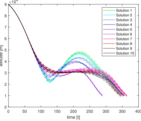
Figure 6 show the time histories of the altitude for all the solutions in the archive, 7 shows the flight path angle and 8 the velocity, with the dashed and dotted lines indicating the 1σuncertainty.

Fig. 6. Altitude vs time

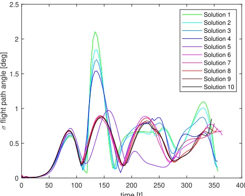
In all these plots it is possible to see that solutions in green, light blue and blue (Solutions 1 to 4) have lower uncer-tainty for the final state. This can also be seen from Figures 9, 10 and 11, which show the standard deviation of altitude,

Fig. 7. Flight path angle vs time

Fig. 8. Velocity vs time

flight path and velocity as a function of time. As previously stated, even if the uncertainty on density is relatively high at high altitudes, its effect is quite limited for the first part of the trajectory. However, it becomes more important as the altitudes get to approximately40 km.

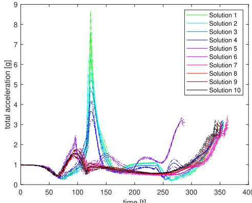
This as the Pareto front was showing, solutions associated with lower uncertainty in final states have higher acceleration loads, as shown in 12.

Fig. 9. Altitude vs time, standard deviations

small negative values, then a sharp increase to values around 10−15 deg, and finally stabilise around0 deglike the other trajectories.

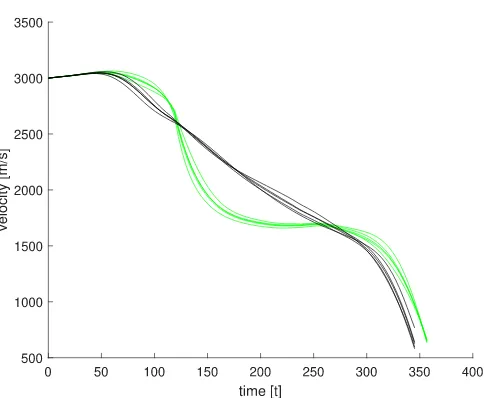
Finally, Figures 14, 15 and 16 show the time history of altitude, flight path angle and velocity of all sigma points for Solution 1 and 10. As it is evident, the green lines have a much lower scattering at the final time than the black lines, indicating that Solution 1 (green) is subject to less uncertainty than solution 10 (black). This figures also give an idea of the complexity of the problem tackled by this approach, where the same control law is applied to multiple independent sigma points (lines with the same colour) and is able to steer the sys-tem to a given expected final state while also reducing the un-certainty associated to the final state, or reducing the expected acceleration load.

6. CONCLUSIONS

This paper presented and extension of MODHOC to perform robust multi-objective optimisation of the reentry trajectories of the Orbital 500R. Employing the Unscented Transforma-tion, a different atmospheric model was developed for each of the sigma points. All the sigma points share the same con-trol law, thus making the trajectory robust against model un-certainty. Albeit only the first two statistical moments of the uncertain values were considered for this work, it is possible to account for higher order moments, making the resulting trajectory even more robust. To this end, however, a larger number of sigma points will be required, and the resulting op-timal control problem becomes progressively larger, requiring the use of large scale optimisation code.

Fig. 10. Flight path angle vs time, standard deviations

7. ACKNOWLEDGEMENTS

This work has been partially funded by the UK Space Agency and European Space Agency (ESA) General Support Tech-nology Programme (GSTP).

8. REFERENCES

[1] Lorenzo A Ricciardi, Massimiliano Vasile, and Christie Maddock, “Global solution of multi-objective optimal control problems with multi agent collaborative search and direct finite elements transcription,” in2016 IEEE Congress on Evolutionary Computation (CEC). IEEE, 2016, pp. 869–876.

[2] Lorenzo A. Ricciardi, Christie A. Maddock, and Massi-miliano Vasile, “Direct solution of multi-objective op-timal control problems applied to spaceplane mission design,” Journal of Guidance, Control and Dynamics, 2018.

[3] Massimiliano Vasile, “Finite elements in time: A direct transcription method for optimal control problems,” in

AIAA/AAS Astrodynamics Specialist Conference, Guid-ance, Navigation, and Control and Co-located Confer-ences, Toronto, Canada, 2-5 Aug 2010.

Fig. 11. Velocity vs time, standard deviations

[5] Lorenzo Angelo Ricciardi, Massimiliano Vasile, Fed-erico Toso, and Christie A Maddock, “Multi-objective optimal control of the ascent trajectories of launch ve-hicles,” inAIAA/AAS Astrodynamics Specialist Confer-ence, 2016, p. 5669.

[6] Massimiliano L Vasile, Christie Maddock, and Lorenzo Ricciardi, “Multi-objective optimal control of re-entry and abort scenarios,” in2018 Space Flight Mechanics Meeting, 2018, p. 0218.

[7] Marilena Di Carlo, Lorenzo Ricciardi, and Massim-iliano Vasile, “Multi-objective optimisation of con-stellation deployment using low-thrust propulsion,” in

AIAA/AAS Astrodynamics Specialist Conference, 2016, p. 5577.

[8] Federico Zuiani, Yasuhiro Kawakatsu, and Massimil-iano Vasile, “Multi-objective optimisation of many-revolution, low-thrust orbit raising for destiny mission,” in23rd AAS/AIAA Space Flight Mechanics Conference, Kauai, Hawaii, 10-14 Feb 2013.

[9] Simon J Julier and Jeffrey K Uhlmann, “A general method for approximating nonlinear transformations of probability distributions,” Tech. Rep., Robotics Re-search Group, Department of Engineering Science, Uni-versity of Oxford, 1996.

[10] I Michael Ross, Ronald J Proulx, Mark Karpenko, and Qi Gong, “Riemann–Stieltjes optimal control problems for uncertain dynamic systems,” Journal of Guidance, Control, and Dynamics, vol. 38, no. 7, pp. 1251–1263, 2015.

Fig. 12. Total acceleration vs time

[11] R. Van der Merwe and E. A. Wan, “The square-root unscented Kalman filter for state and parameter-estimation,” in2001 IEEE International Conference on Acoustics, Speech, and Signal Processing Proceedings (Cat. No.01CH37221). IEEE.

[12] Peter Zipfel,Modeling and Simulation of Aerospace Ve-hicle Dynamics, Second Edition, AIAA Education Se-ries, 2007.

[13] Christie Alisa Maddock, Lorenzo Ricciardi, Michael West, Joanne West, Konstantinos Kontis, Sriram Ren-garajan, David Evans, Andy Milne, and Stuart McIn-tyre, “Conceptual design analysis for a two-stage-to-orbit semi-reusable launch system for small satellites,”

Acta Astronautica, vol. 152, pp. 782–792, 2018.

[14] NASA NOAA and US Air Force, “US Standard At-mospheres,”Washington, DC: US Government Printing Office, pp. 53–63, 1976.

Fig. 13. Angle of attack vs time

Fig. 14. Time history of the altitude for all sigma points of Solutions 1 and 10

Fig. 15. Time history of the flight path angle for all sigma points of Solutions 1 and 10