Effect of anisotropy and destructuration on behavior of Haarajoki test embankment

Effect of Anisotropy and Destructuration on Behavior of

Haarajoki Test Embankment

Abdulazim Yildiz

; Minna Karstunen

; and Harald Krenn

Abstract:This paper investigates the influence of anisotropy and destructuration on the behavior of Haarajoki test embankment, which was built by the Finnish National Road Administration as a noise barrier in 1997 on a soft clay deposit. Half of the embankment is constructed on an area improved with prefabricated vertical drains, while the other half is constructed on the natural deposit without any ground improvement. The construction and consolidation of the embankment is analyzed with the finite-element method using three different constitutive models to represent the soft clay. Two recently proposed constitutive models, namely S-CLAY1 which accounts for initial and plastic strain induced anisotropy, and its extension, called S-CLAY1S which accounts, additionally, for interparticle bonding and degradation of bonds, were used in the analysis. For comparison, the problem is also analyzed with the isotropic modified cam clay model. The results of the numerical analyses are compared with the field measurements. The simulations reveal the influence that anisotropy and destructuration have on the behavior of an embankment on soft clay.

DOI:10.1061/共ASCE兲1532-3641共2009兲9:4共153兲

CE Database subject headings:Embankments; Anisotropy; Destruction; Finite element method; Drainage.

Introduction

In many regions of the world, population growth, economic needs, and environmental constraints necessitate construction of structures on soft clay deposits, which were considered unsuitable for construction just a couple of decades ago. Modeling of soft clays has always been one of the main focuses in geotechnical engineering. The stress-strain behavior of natural soft soils is highly nonlinear and very complex, as different fundamental fea-tures of soil, such as anisotropy, creep, and destructuration, influ-ence its response to foundation loading. Current geotechnical design practice routinely relies on simplified theories, and the methods used are at best very crude and conservative共and hence uneconomical兲, or at worst unsafe.

Advanced geotechnical design on soft clays has often been based on finite-element analyses using isotropic elasto-plastic soil models, such as modified cam clay共Roscoe and Burland 1968兲

and its isotropic extensions. Natural clays, however, are highly anisotropic because of the mode of their sedimentation, the pre-ferred orientation of plate-shaped clay particles during deposition, and the subsequent consolidation under self-weight loading

共Tavenas and Leroueil 1977; Ladd et al. 1977; Diaz-Rodriguez et al. 1992兲. Anisotropy can influence both elastic and plastic

behavior. For normally consolidated or lightly overconsolidated soft clays, plastic deformations are likely to dominate for many problems, such as the embankment loading considered in this paper. Most natural clays are structured 共Leroueil and Vaughan 1990; Burland 1990兲, which reflects the soil composition, history, present state, and environment. The structure is composed of fab-ric共the geometrical arrangement of soil particles and particle con-tacts兲, which is often anisotropic, and some form of apparent interparticle bonding. Interparticle bonding results from the min-eralogy and pore-water composition combined with complex geo-chemical processes, and it gives the soil additional resistance to yielding. Plastic straining modifies the anisotropy, and gradually breaks the apparent bonding, due to slippage at interparticle con-tacts and subsequent rearrangement and realignment of particles. The degradation of bonding due to plastic strains is referred to as destructuration, and it significantly affects the mechanical behav-ior of soft clays 共Rouainia and Muir Wood 2000; Leroueil and Vaughan 1990兲. Indeed, the mechanical behavior of natural soils is controlled by the bond degradation and the intrinsic properties of the soils共Burland 1990兲.

When constructing embankments on soft compressible soils with low bearing capacity and low hydraulic conductivity, the stability and time required for consolidation are the two major considerations in the design 共Li and Rowe 2002兲. Prefabricated vertical drains共PVDs兲are commonly used to shorten the consoli-dation times on thick soft deposits by providing short horizontal drainage paths共Jamiolkowski et al. 1983兲. The PVD is a slender, synthetic drainage element comprised of a drainage core wrapped in a geotextile filter. However, in recent years, the technique of reinforcing the embankment at the base using geosynthetic rein-forcement to improve its short-term stability has become popular

Taechakumthorn 2007兲. PVDs also work together with geosyn-thetic reinforcement to minimize the differential settlement and lateral deformation of the foundation and the combined use of the geosynthetic reinforcement and PVDs enhances embankment per-formance substantially more than the use of either method of soil improvement alone共Rowe and Taechakumthorn 2008兲.

The finite-element method共FEM兲is often used for predicting the performance of embankments constructed on soft soils and extensive research has been carried out in this area for the past several years共Rowe and Soderman 1984; Schaefer and Duncan 1988; Hird and Kwok 1989; Sanchez and Sagaseta 1990; Chai and Bergado 1993; Bergado et al. 1995; Indraratna and Redana 1997, 2000; Borges et al. 2000; Neher et al. 2001; Bergado et al. 2002; Shen et al. 2005; Karstunen et al. 2005; Gnanendran et al. 2006兲. Isotropic elasto-plastic models 共Roscoe and Schofield 1963; Roscoe and Burland 1968; Chen 1982兲 have been com-monly used successfully to predict the behavior of embankment. However, it was concluded that even allowing for consolidation, these models was not adequate for accurately and simultaneously predicting multiple characteristics of the embankment behavior

共e.g., vertical and horizontal deformations, pore pressure兲. Ne-glecting the effects of anisotropy and/or destructuration may lead to inaccurate predictions of soft clay response 共Karstunen et al. 2005兲. Due to the viscous nature of some soft clayey foundations, the time dependency of stress-strain behavior of soft clays also has a significant influence on the behavior of embankments. For example, Rowe et al. 共1996兲 showed that in order to accurately predict the responses of the Sackville test embankment on a rate sensitive soil, it was essential to consider the effect of soil viscos-ity. Rowe and Hinchberger共1998兲proposed an elasto-viscoplastic constitutive model and demonstrated that the proposed model could adequately describe the behavior of the Sackville test em-bankment. Therefore, there is a need for a constitutive model that can adequately account for fundamental features of soil, such as anisotropy, destructuration, and creep in a relatively simple manner.

In recent years there have been considerable developments in understanding the behavior of soft clays and a number of elasto-plastic constitutive models incorporating features such as aniso-tropy and/or destructuration have been published in the literature

共Whittle and Kavvadas 1994; Kavvadas and Amorosi 2000; Rouainia and Muir Wood 2000; Liu and Carter 2002; Nova et al. 2003; Dafalias et al. 2006兲. Most of these models, however, do not take into account the combined effect of anisotropy and de-structuration. Furthermore, the application of these models to practical geotechnical design is not common, because the deter-mination of the model input parameters is often cumbersome, and it may even require nonstandard laboratory tests.

The S-CLAY1 model proposed by Wheeler et al.共2003兲is an elasto-plastic model that attempts to provide a realistic represen-tation of the influence of plastic anisotropy while still keeping the model relatively simple. The model parameters can be determined from the results of standard laboratory tests by using well-defined methodologies. Furthermore, the model has been successfully validated against experimental data on several natural and recon-stituted clays 共Koskinen et al. 2002a, b; Wheeler et al. 2003, Karstunen and Koskinen 2008兲. The extension of the model called S-CLAY1S 共Karstunen et al. 2005兲 incorporates the combined effect of anisotropy, bonding, and destructuration. S-CLAY1S ac-counts for the additional strength given by the apparent bonds with a so-called intrinsic yield curve, a concept originally pro-posed by Gens and Nova 共1993兲. In this study, the S-CLAY1

共Wheeler et al. 2003兲 and S-CLAY1S 共Karstunen et al. 2005兲

models are applied to represent the soft clay under Haarajoki test embankment in Finland. The results of numerical studies are com-pared with field observations. For comparison, the problem is also analyzed with the isotropic modified cam clay model共Roscoe and Burland 1968兲.

The true modeling of an embankment with vertical drains re-quires three-dimensional 共3D兲 analyses. Most analyses however have adopted plane strain conditions. The problem of water flow into a vertical drain under an infinitely wide fill is axisymmetric, and therefore the vertical drain system must be converted into an equivalent plane strain model for numerical simulations. Several authors共Hird et al. 1992, 1995; Chai et al. 1995, 2001; Indraratna and Redana 1997兲have shown that vertical drains can be effec-tively modeled by using appropriate mapping methods to repre-sent the typical arrangement of vertical drains in plane strain finite-element analyses. However, certain simplifying assump-tions are made, as discussed later on. The two most useful map-ping approaches from a computational point of view are those by Chai et al. 共2001兲 and Hird et al.共1992兲, as accounting for the effects of the smear zones around the drains does not require separate discretization. In this paper the combined mapping pur-posed by Hird et al.共1992兲is used in the analysis of the behavior of PVD improved subsoil in combination with complex elasto-plastic models, namely MCC, S-CLAY1, and S-CLAY1S.

First, a brief description of constitutive models is given, fol-lowed by information about the embankment geometry, material parameters, and initial conditions, as necessary for the input of numerical analyses. Finally, the results of numerical analyses of Haarajoki embankment on soft clay deposit with and without PVD improvement are compared with the corresponding field observations.

Constitutive Models

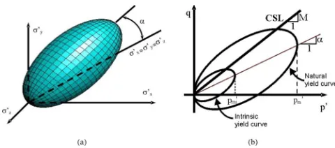
The S-CLAY1S model is a critical state model with anisotropy of plastic behavior represented through an inclined yield surface and a hardening law to model the development or erasure of fabric anisotropy during plastic straining. Additionally, the model ac-counts for destructuration. In three-dimensional stress space the yield surface of the S-CLAY1S model is a sheared ellipsoid

关Fig. 1共a兲兴, given by

f=3₂关兵␴_d−p⬘␣_d其T兵␴_d−p⬘␣_d其兴−

关

兴

= 0 共1兲

where␴_d= deviatoric deviatoric stress tensor;p⬘= mean effective

stress;␣_d= deviatoric fabric tensor共a dimensionless second-order

see Wheeler et al. 2003 for details兲;M= value of the stress ratio at critical state; and p_m⬘ defines the size of the yield surface of the natural clay. Eq. 共1兲 shows that the generalized version of the yield surface cannot be expressed solely in terms of stress invari-ants. Fig. 1共a兲illustrates the shape of the S-CLAY1S yield surface in three-dimensional stress space, for the case where the principal axes of both the stress tensor and the fabric tensor coincide with thex,y, andzdirections.

Within the yield surface there is a notional “intrinsic yield surface” for the equivalent unbonded soil with the same fabric, which is assumed to be of the same shape and orientation as the real yield surface, but smaller in size. The size of the intrinsic yield surface is specified by a parameterp_mi⬘, and this is related to the sizep_m⬘of the yield surface for the natural soil by parameter␹, defining the current degree of bonding

pm⬘=共1 +␹兲pmi⬘ 共2兲

For the simplified conditions of a triaxial test on a previously one-dimensionally consolidated sample, it can be assumed that the horizontal plane in the triaxial sample coincides with the plane of isotropy of the sample. In this special case, the fabric tensor can be replaced by a scalar parameter␣, defined as

␣2₌3

2兵␣d其T兵␣d其 共3兲 which is a measure of the degree of plastic anisotropy of the soil. The yield curves of the S-CLAY1S model can then be visualized by Fig. 1共b兲. For the sake of simplicity, the S-CLAY1S model assumes isotropic elastic behavior, of the same form as in the

modified cam clay model 共Roscoe and Burland 1968兲, and an associated flow rule.

S-CLAY1S incorporates three hardening laws. The first of these relates the change in the size of the intrinsic yield surface to the plastic volumetric strain incrementd␧v

p

dp_mi⬘ = vpmi⬘

␭_i−␬d␧v

p _共4兲

where␭i= gradient of the intrinsic normal compression line共for a reconstituted soil兲 in the lnp_⬘-v plane 共where v= specific

vol-ume兲. Eq.共4兲is of the same form as the equivalent hardening law in MCC and S-CLAY1, but with p_m⬘ replaced by p_mi⬘ and ␭ re-placed by␭_i.

The second hardening law 共the rotational hardening law兲 de-scribes the change of orientation of the yield surface with plastic straining共Wheeler et al. 2003兲

d␣_d=␻

冉

冋

3␩

4 −␣d

册

d

冋

␩

3−␣d

册

p

冊

where␩=␴_d/_p⬘;d␧

d

p_{= increment of plastic deviatoric strain; and}

␻and␻_d= additional soil constants. The soil constant␻_dcontrols the relative effectiveness of plastic shear strains and plastic volu-metric strains in setting the overall instantaneous target values for the components of ␣d, whereas the soil constant␻ controls the absolute rate of rotation of the yield surface toward the current target values of the components of␣_d共see Wheeler et al. 2003 for

details兲. (a)

(b)

2.9 m

2 m

20.2 m

2 - 3 m 2 - 3 m

100 m

Vertical strip drains c/c 1.0 m CLAY

Cu = 14 - 30 kN/m² W = 70 - 110 % Ip = 45 - 75 % DRY CRUST

SILT

TILL SOFT SOIL DEPOSIT

3

584

0

3

588

0

2.9 m 1:2 1:2

8 m

The third hardening law in S-CLAY1S 共the destructuration law兲describes the degradation of bonding with plastic straining. It is similar in form to the rotational hardening law 关Eq. 共5兲兴, except that both plastic volumetric strains and plastic shear strains

共whether positive or negative兲tend to decrease the value of the

bonding parameter␹toward a target value of zero

d␹=␰共关0 −␹兴兩d␧v p_兩+␰

d关0 −␹兴d␧d

p_{兲= −␰␹共兩d␧} v p_兩+␰

dd␧d p_{兲 共6兲}

where ␰ and␰_d= additional soil constants. Parameter ␰ controls the absolute rate of destructuration, and parameter␰_dcontrols the

35840 35880

B1

B3

B4

B5 -4m

-7m

-10m

-15m +/-0m

GWT 100 m

20 m

3m

20

m

2

-3

m

2-3

m

SILT

TILL -2m

-6m

B : Piezometer B2

I1

I2 P20

P19

V

ert

ic

al

drai

ned

area

P10 P8

P11

P12 P9

P16

P17 P18

I3

I4

I:Inclinometers

P:Settlement plates

I5

35840 35880

relative effectiveness of plastic deviatoric strains and plastic volu-metric strains in destroying the bonding 共see Koskinen et al. 2002a for details兲. Theoretically, as pointed out in Zentar et al.

共2002兲, a monotonic reduction in␹implied by the hardening law

关Eq.共6兲兴can sometimes result in reduction ofpm⬘ during harden-ing for certain combinations of parameters ␰, ␰d, and ␹. As a result, the peak undrained shear strength of the natural soil may actually be predicted to decrease during consolidation. There is field evidence for such behavior on a moderately sensitive Finnish clay, as discussed in Karstunen et al.共2005兲.

By setting the initial value of the state parameter␹to zero and using an apparent value of␭共determined from an oedometer test on a natural clay sample兲, instead of the intrinsic value ␭_iof a reconstituted clay, S-CLAY1S reduces to the S-CLAY1 model that accounts for plastic anisotropy only. Furthermore, if in addi-tion the initial value of the state parameter␣共used for calculating the initial values of the components of the fabric tensor兲and the value of the soil constant␻are set to zero, the model ultimately reduces to the isotropic modified cam clay共MCC兲model.

Haarajoki Test Embankment

In 1997 the Finnish National Road Administration organized an international competition to predict the stress-strain behavior of a road embankment in Haarajoki, Finland. The embankment is founded on soft soil deposits which are typical for the region

共FinnRA 1997兲, and can be characterized by a high degree of anisotropy and natural interparticle bonding, which reflect in geo-technical properties, such as the permeability, stress-strain rela-tionship, and shear strength. Half of the embankment is constructed on an area improved with prefabricated vertical

drains and the other half is constructed on natural deposits with-out any additional ground improvement. The data concerning site investigation and results of the associated laboratory tests and field monitoring data provided by FinnRA共1997兲are very useful for the validation of different constitutive models and methods of analyses. Results of finite-element studies of the embankments have been published, by Aalto 共1998兲, Näätänen et al. 共1998兲, Cudny and Neher 共2003兲, and most recently by Zhou and Yin

共2004兲. The results of the competition to calculate the settlement of the embankment have been summarized in Lojander and Ve-psäläinen共2001兲. The analyses by Aalto共1998兲and Näätänen et al.共1998兲were small strain analyses which assumed the soil to be isotropic, similarly to Zhou and Yin共2004兲 who also accounted for creep. Cundy and Neher共2003兲utilized the so-called multil-aminate framework to represent the soft soil. Their model ac-counted for anisotropy and destructuration via directionally distributed overconsolidation. This approach is, however, rather complex and difficult to justify, and furthermore the multilami-nate models are computationally demanding and difficult to vali-date experimentally. In this paper the phenomena of anisotropy and destructuration are represented via the S-CLAY1S model, which is relatively easy to understand and, most importantly, ex-perimentally validated for a number of natural clays 共Koskinen et al. 2002a; Zentar et al. 2002; Karstunen and Koskinen 2004兲.

Geometry and Ground Conditions

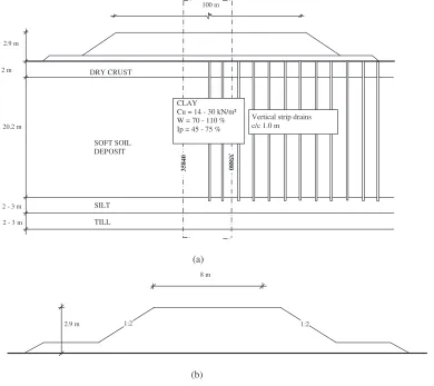
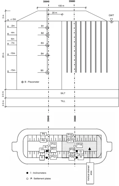
The longitudinal profile and the cross section of Haarajoki test embankment are shown in Fig. 2. The embankment is 2.9 m high and 100 m long, 8 m wide, and the slopes have a gradient of 1:2. The embankment itself was constructed in 0.5 m thick layers and each layer was applied and compacted within 2 days. In the im-proved area the vertical drains were installed in a regular pattern with 1 m spacing before embankment construction. Numerous measuring devices共settlement plates, piezometers, inclinometers, pressure cells兲 were installed under the test embankment for monitoring the vertical and lateral displacements and the pore pressures. The layout of some of these instruments is presented in Fig. 3 and the depths and locations of these instruments are sum-marized in Table 1.

Haarajoki test embankment is founded on a 2 m thick dry crust layer overlying a 22.2 m thick soft clay deposit. The layers below the soft clay consist of silt and till material, based on cone penetration tests 共CPTs兲, and can be considered as permeable

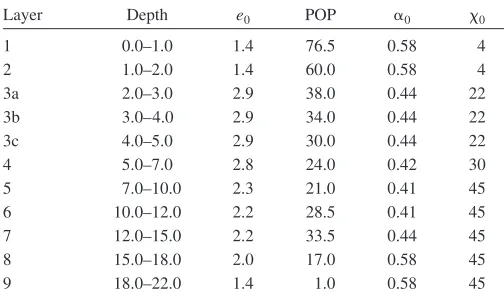
共FinnRA 1997兲. The groundwater table is at the ground surface. The subsoil is divided into nine sublayers with different com-pressibility parameters and overconsolidation ratios. The water

Table 1. Depths and Locations of Instruments under Haarajoki Test Embankment

Instruments Chainage

Location共from centerline兲

Depth 共m兲

Settlement plates

P8 35840 9 m left —

P9 35840 4 m left —

P10 35840 Centerline —

P11 35840 4 m right —

P12 35840 9 m right —

P16 35880 9 m left —

P17 35880 4 m left —

P18 35880 Centerline —

P19 35880 4 m right —

P20 35880 9 m right —

Piezometer tips

B1 35837 Centerline 2

B2 35837 Centerline 4

B3 35837 Centerline 7

B4 35837 Centerline 10

B5 35837 Centerline 15

Inclinometers

I1 35838 4 m right —

I2 35838 9 m right —

I3 35882 4 m right —

I4 35882 9 m right —

I5 35838 4 m right —

Table 2.Haarajoki Test Embankment; Initial Values for State Parameters

Layer Depth e0 POP ␣0 ␹0

1 0.0–1.0 1.4 76.5 0.58 4

2 1.0–2.0 1.4 60.0 0.58 4

3a 2.0–3.0 2.9 38.0 0.44 22

3b 3.0–4.0 2.9 34.0 0.44 22

3c 4.0–5.0 2.9 30.0 0.44 22

4 5.0–7.0 2.8 24.0 0.42 30

5 7.0–10.0 2.3 21.0 0.41 45

6 10.0–12.0 2.2 28.5 0.41 45

7 12.0–15.0 2.2 33.5 0.44 45

8 15.0–18.0 2.0 17.0 0.58 45

content of the soft clay layer varies between 75 and 112% de-pending on the depth, and is almost the same as, or greater than, the liquid limit. The bulk density varies from 14 to 17 kN/_m3_and specific gravity varies from 2.73 to 2.79. The undrained共 undis-turbed兲shear strength was determined by fall cone tests and field vane tests to be between 15 and 42 kN/_m2共FinnRA 1997兲. The Haarajoki deposits can be characterized as a sensitive anisotropic soft soil with sensitivity values共determined with fall cones tests兲

between 20 and 55. The organic content is between 1.4 and 2.2% at a depth of 3 – 13 m. Some typical characteristics of the deposits are shown in Fig. 4.

Input Data for Numerical Analyses

The embankment, which was made of granular fill, was modeled with a simple Mohr–Coulomb model assuming the following ma-terial parameters:E_⬘= 40,000 kN/_m2_{,␯⬘= 0.35,␾⬘= 40°,␺⬘= 0°,}

c_⬘= 2 kN/_m2_{, and} ␥= 21 kN/_m3 共where E_⬘= Young’s modulus;

␯_⬘= Poisson’s ratio; ␾_⬘= friction angle; ␺_⬘= dilatancy angle; and

␥= unit weight of the embankment material兲. The problem is dominated by the soft clay response and is hence rather insensi-tive to the embankment parameters.

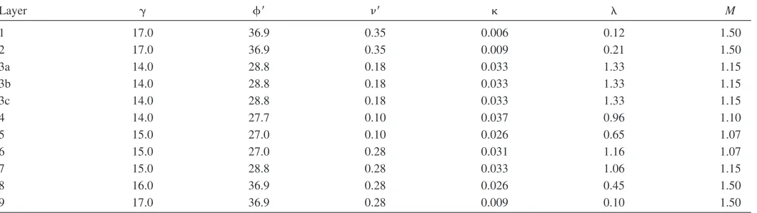
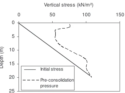
The soft clay deposit was modeled as a lightly overconsoli-dated soft clay with vertical preconsolidation pressures varying with the depth as shown in Fig. 5 and Table 2. In the analyses the preconsolidation is modeled via vertical preoverburden pressure 共POP兲=␴_p⬘−␴v0⬘共where␴v0⬘and␴p⬘are, respectively, the in situ value and maximum past value of the vertical effective stress兲. The in situ stresses were calculated by assuming a horizontal effective stress distribution, using K0 values estimated with the equation K0=共1 − sin␾⬘兲OCRsin␾⬘ 共Mayne and Kulhawy 1982兲, where␾_⬘= critical state friction angle in triaxial compression and OCR= vertical overconsolidation ratio共OCR=␴_p⬘/_␴

v0_⬘兲. The val-ues of the input parameters and state variables for the models are listed in Tables 2–4. The values of soil parameters were estimated for each layer based on laboratory results provided by FinnRA

共1997兲using the best practice for the determination of model and state parameters for the S-CLAY1S model and its simplifications

共i.e., S-CLAY1 and MCC兲. Due to natural variability, there was some scatter in the values and for each layer average values have been chosen. The values of permeability used for calculations were reported by Näätänen et al. 共1998兲 based on vertical and horizontal constant rate of strain 共CRS兲 oedometer tests. In the finite-element analyses, the decrease in the permeability as the void ratio decreases was taken into account using the formula by Taylor共1948兲

log

冉

冊

=⌬e ck

共7兲

where⌬e= change in void ratio;k= soil permeability in the cal-culation step; k0= initial value of the permeability; and ck= permeability change index. It was assumed thatck= 0.5e0in the calculations共Tavenas et al. 1983兲. The use of the S-CLAY1 model requires values of six soil constants 共␭,␬,␯_⬘,M,␻, and

␻d兲and information on initial state共initial values for void ratioe0,

␣0, andpm⬘兲. The values of␬and␭were determined from oedom-eter test results. The values for the initial inclination ␣₀ of the yield surface and parameter ␻_d were determined following the procedure described by Wheeler et al. 共2003兲, usingK₀NCvalues corresponding to Jaky’s simplified formula. The values of␻were estimated based on apparent values of␭, as suggested by Zentar et al.共2002兲. The use of the S-CLAY1S model requires, addition-ally, values for the two destructuration parameters共␰and␰_d兲and information on the initial amount of bonding␹₀. The values of␭_i

need to be measured from oedometer tests on reconstituted samples. In the absence of these tests, ␭ivalues were estimated throughout the deposit assuming similar␭/_␭

iratios to other Finn-ish clays, and similarly, past experience on FinnFinn-ish clays was used in fixing the values for parameters␰and␰_dthat control the rate of degradation of bonding. The initial values of ␹0 were estimated based on sensitivity, as suggested in Koskinen et al.

共2002a兲. Therefore, in the following simulations, it is possible to do quantitative comparisons between the isotropic MCC model and the anisotropic S-CLAY1 model, but the comparisons be-tween these models and the S-CLAY1S model are generally qualitative rather than quantitative, given not enough data were available for determination of the key constants controlling the rate of destructuration.

Numerical Analyses and Comparisons with Observations

In order to investigate the influence of anisotropy and destructu-ration on the behavior of an embankment on Haarajoki deposits, the construction and consolidation of Haarajoki test embankment on soft soils with and without vertical drains were simulated with different constitutive models共MCC, S-CLAY1, and S-CLAY1S兲

using PLAXIS 2D Version 8.2共Brinkgreve 2002兲. These consti-tutive models have been implemented in the finite-element pro-gram as user-defined models by Wiltafsky共2003兲. The results of the numerical analyses were compared with the field

measure-Table 3.Haarajoki Test Embankment; Values for MCC Soil Constants

Layer ␥ ␾_⬘ ␯_⬘ ␬ ␭ M

1 17.0 36.9 0.35 0.006 0.12 1.50

2 17.0 36.9 0.35 0.009 0.21 1.50

3a 14.0 28.8 0.18 0.033 1.33 1.15

3b 14.0 28.8 0.18 0.033 1.33 1.15

3c 14.0 28.8 0.18 0.033 1.33 1.15

4 14.0 27.7 0.10 0.037 0.96 1.10

5 15.0 27.0 0.10 0.026 0.65 1.07

6 15.0 27.0 0.28 0.031 1.16 1.07

7 15.0 28.8 0.28 0.033 1.06 1.15

8 16.0 36.9 0.28 0.026 0.45 1.50

Table 4.Haarajoki Test Embankment; Values for Additional Soil Con-stants for S-CLAY1 and S-CLAY1S

Layer ␻d ␻ ␭i ␰ ␰d

1 1.00 50 0.04 8 0.2

2 1.00 50 0.06 8 0.2

3a 0.70 20 0.38 8 0.2

3b 0.70 20 0.38 8 0.2

3c 0.70 20 0.38 8 0.2

4 0.64 20 0.27 8 0.2

5 0.60 20 0.19 8 0.2

6 0.60 20 0.33 8 0.2

7 0.70 20 0.30 8 0.2

8 1.00 20 0.13 8 0.2

9 1.00 20 0.03 8 0.2

0

5

10

15

20

25

0 1 2 3

Organic matter (%)

De

pt

h

(m

)

0

5

10

15

20

25

10 12 14 16 18 20

Bulk density (kN/m³)

0

5

10

15

20

25

0 25 50 75 100

Undrained shear strength (kPa)

(a)

(b)

(c)

0

5

10

15

20

25

0 25 50 75 100

Sensitivity (-)

0

5

10

15

20

25

0 25 50 75 100 w (%)

D

ep

th(

m

)

wP wL

w

0

5

10

15

20

25

0 25 50 75 100

Clay Content (%)

(d)

(e)

(f)

Fig. 4.Typical soil characteristic of Haarajoki deposit

0

5

10

15

20

25

0 50 100 150

Vertical stress (kN/m²)

D

ept

h

(m

)

Initial stress

Pre-consolidation pressure

ments. A cross section of the embankment built on soft clay with-out vertical drains 共Cross Section 35840兲 was firstly simulated and then a cross section within the vertically drained area共Cross Section 35880兲was simulated.

Cross Section 35840

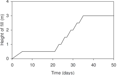
The Cross Section 35840 is situated on the natural deposits with-out any ground improvement. The test embankment was assumed symmetric and only half of the embankment is considered in the finite-element analyses. The plane strain condition and six-noded triangular elements were used and all simulations were done as large strain analyses. A finite-element mesh with 833 elements is used to model the subsoil and the embankment. The groundwater table is located at the ground surface. The lateral boundaries are restrained horizontally, and the bottom boundary is restrained in both directions. Drainage boundaries are assumed to be at the ground surface and at the bottom of the mesh, whereas the lateral boundaries are closed. The embankment construction consists of two phases: first, the embankment loading is applied under und-rained conditions, assuming the embankment to be dund-rained mate-rial and next, a consolidation phase is simulated via fully coupled consolidation analysis. The construction of Haarajoki embank-ment was done in 0.5 m layers, each taking 2 days, while the foundation layer was constructed in 5 days, and the real construc-tion schedule has been simulated in the calculaconstruc-tion共Fig. 6兲. After the construction of each layer a consolidation phase is introduced to allow the excess pore pressures to dissipate. Hence, a total of 12 calculation phases were defined in the analyses. The construc-tion of embankment was completed in 35 days. After construcconstruc-tion of the last layer, the calculations have been taken until the excess pore pressure had dissipated to a residual value of 1 kPa to deter-mine the final consolidation settlement. Mesh sensitivity studies were done to confirm that the mesh was dense enough to give accurate results for all of the constitutive models concerned.

The observed and predicted vertical settlements versus time at a node directly under the centerline and the crest of the embank-ment are presented in Fig. 7. Differences between the three mod-els are relatively minor immediately after construction of the embankment, but become significant during consolidation. The measured settlement underneath the centerline of the embankment is 0.46 m after about 5 years of consolidation. The MCC model predicts a vertical displacement of about 0.33 m after 5 years of consolidation underneath the centerline of the embankment, while the S-CLAY1 and S-CLAY1S models predict vertical displace-ments of about 0.43 and 0.49 m, respectively关Fig. 7共a兲兴. The final value of settlement underneath the crest, corresponding to about

5 years of consolidation, is measured to be 0.39 m. The vertical displacements underneath the crest are predicted by S-CLAY1 and S-CLAY1S models to be 0.36 m and 0.38 m, respectively while the MCC model predicts as about 0.28 m after about 5 years of consolidation关Fig. 7共b兲兴. The predictions of the verti-cal displacements by the two anisotropic models共S-CLAY1 and S-CLAY1S兲are in good agreement with field observations. The isotropic MCC model predicts notably smaller settlements than the observed ones. The S-CLAY1S model predicts marginally larger vertical settlements than the S-CLAY1 model. Both the calculated and observed time-settlement curves suggest that the primary consolidation is still continuing after 2,000 days, which corresponds to the last measurement data available.

The predicted surface settlements corresponding to a time im-mediately after construction and after 5 years of consolidation are shown in Fig. 8. The measurements demonstrate that assuming symmetry was justified. All models predict small amounts of sur-face heave outside the embankment immediately after construc-tion关Fig. 8共a兲兴and a maximum vertical settlement underneath the centerline of the embankment. The maximum vertical settlement measured underneath the centerline of the embankment is about 0.46 m after 5 years of consolidation. The MCC model predicts a vertical displacement of about 0.33 m after 5 years of consolida-tion, while the S-CLAY1 and S-CLAY1S models predict vertical displacements of about 0.43 and 0.49 m, respectively关Fig. 8共b兲兴. Again it can be seen that both anisotropic models are in good agreement with the observed surface settlements.

The vertical displacements at different depths underneath the centerline of the embankment predicted by three constitutive

0 1 2 3 4

0 10 20 30 40 50

Time (days)

H

e

ig

h

to

f

fill

(m

)

Fig. 6.Haarajoki test embankment; construction schedule

0,0

0,1

0,2

0,3

0,4

0,5

0,6

0,7

0 500 1000 1500 2000 2500

Time (days)

S

et

tl

em

en

t

(m

)

Observed MCC S-CLAY1 S-CLAY1S

(a)

0,0

0,1

0,2

0,3

0,4

0,5

0,6

0,7

0 500 1000 1500 2000 2500

Time (days)

S

et

tl

em

en

t

(m

)

Observed (right) Observed (left) MCC S-CLAY1 S-CLAY1S

(b)

models are presented in Fig. 9 against time. Unfortunately, no extensometer results were available for comparison. SCLAY1S predicts larger vertical settlements than the S-CLAY1 and MCC models within the dry crust layer. At a depth of 2 m, the values of settlements obtained from the S-CLAY1 and S-CLAY1S models are very similar. However, the S-CLAY1 model predicts larger settlements than the S-CLAY1S and MCC models from a depth of 2 m downwards. This is due to the predicted rate of destructura-tion, which depends on the values assumed for soil constants␭_i,

␰, and ␰_d 共which were chosen based on experience rather than directly derived from laboratory data兲, the initial amount of bond-ing共␹0兲, as well as the stress ratio. In the normally consolidated range, the predicted stress ratio depends on the input values forM

共or␾_⬘兲for the anisotropic S-CLAY models. For high stress ratio

共lowK0兲, destructuration is rapid, and hence the values of appar-ent ␭ are high and the settlements predicted by S-CLAY1S are large at shallow depths. For nearly isotropic stress paths, the de-structuration would be slow and the apparent values of ␭ are rather low. In the case of Haarajoki embankment, the value of normally consolidatedK0 increases with depth up to a depth of 12 m. With the chosen set of parameters, the effect of anisotropy overall seems to be more dominant than destructuration共see Fig. 7兲, but as demonstrated in Fig. 7, this is not necessarily true with depth. It should be noted again that the results by S-CLAY1S in Fig. 9 are qualitative rather than quantitative but demonstrate the complex effect of destructuration on natural clays. Based on Fig. 9, it would be good practice for any test embankments to have extensometers installed in order to be able to fully validate con-stitutive models.

The horizontal displacements predicted by the MCC, S-CLAY1, and S-CLAY1S models underneath the crest of the embankment 共4 m from the centerline兲 after 1 and 3 years of consolidation are compared with the measured values in Figs. 10共a and b兲. After 1 year of consolidation the predictions by the anisotropic models 共S-CLAY1 and SCLAY1S兲are closer to the

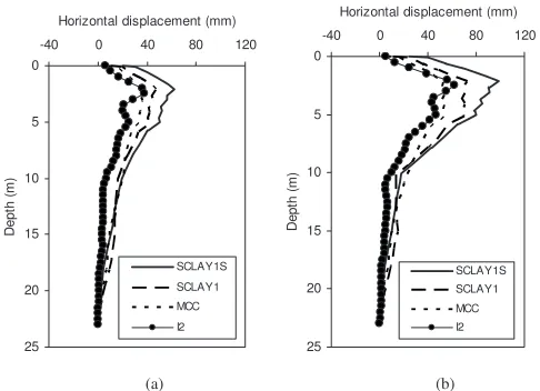
measured results than the prediction by the MCC model. The horizontal displacements after 3 years of consolidation predicted by the SCLAY1 model are again in good agreement with the measured ones关Fig. 10共b兲兴. The MCC model underestimates the horizontal displacements up to a depth of 5 m. The measured maximum horizontal displacement is about 0.076 m and it occurs at a depth of about 2.5 m. The S-CLAY1 model predicts the maximum value as 0.067 m, in contrast to 0.042 m by the MCC model. The scatter in the measurements in Fig. 10 is notable, in particular at great depths, and the reason for this is that the origi-nal inclinometer I1 was destroyed during construction, and I5 was later on added as a replacement. The values in Fig. 10 are the sum of I1 displacements at a particular time with I5 results. One may therefore question the reliability of the field measurements under the crest of the embankment. Fortunately these are not as apparent under the toe of the embankment. Fig. 11 shows a comparison of the measured horizontal displacements with the predicted hori-zontal displacements underneath the toe of the embankment

共about 9 m from the centerline兲. The MCC model gives a margin-ally better prediction of horizontal displacements underneath the toe of the embankment than S-CLAY1, despite of the poor pre-diction of vertical displacements in Fig. 7. Again the measured maximum horizontal displacement occurs at a depth about 2.5 m and is about 0.062 m. As seen from Figs. 10 and 11, the MCC model overall predicts lower values of horizontal displacements than the two anisotropic models and notably smaller vertical de-formations共Fig. 7兲than the anisotropic models. Consequently, the isotropic model predicts a much higher ratio of horizontal to ver-tical displacements than the anisotropic models. The depth of the maximum horizontal displacement was well predicted by all mod-els considered. All modmod-els seem to overpredict the horizontal dis-placements between 5 and 15 m depths, and the measured horizontal displacements are very small, or approximately zero, after 15 m depth.

The predicted and measured excess pore pressure values at different depths under the centerline of the embankment are com-pared in Fig. 12. As expected, the excess pore pressures increase during the embankment construction and then gradually dissipate with time. The predicted excess pore pressures are in general higher than the measured ones. The calculated excess pore pres-sure values correspond quite well with the meapres-surements at depths of 10 and 15 m, while the predicted values at 4 and 7 m depths are greater than the measured values. This can be partly explained by the fact that the excess pore pressures are strongly influenced by the foundation soil permeability. The values of per-meability used in the analyses were calculated directly from CRS oedometer test results. Laboratory tests normally underestimate the field values of permeability. The other reason for the discrep-ancies of predicted and measured excess pore pressures might be due to possible errors in measurements or their interpretation, and/or due to ignoring the effects of creep in the simulations.

Cross Section 35880„PVD Improved Area…

Cross section 35880 is situated in the middle of the part of Haara-joki test embankment constructed on soft clay improved with PVDs共Fig. 2兲. The length of the vertical drains is 15 m and they were installed in a square grid with 1 m spacing underneath the embankment. The drain parameters relevant for the analysis are summarized in Table 5. The prefabricated drains have a typical rectangular cross section and were converted to be equivalent to a circular drain having a diameterdwof 67 mm based on “perimeter equivalence” proposed by Hansbo共1979兲

-0,05

0,00

0,05

0,10

0,15

0,20

0 10 20 30 40

Distance from symmetry axis (m)

S

et

tl

em

ent

(m

)

S-CLAY1S S-CLAY1 MCC Observed (left) Observed (right)

(a)

-0,1

0,0

0,1

0,2

0,3

0,4

0,5

0 10 20 30 40

Distance from symmetry axis (m)

S

e

ttl

e

m

e

n

t

(m

)

S-CLAY1S S-CLAY1 MCC Observed (left) Observed (right)

(b)

0,0 0,1 0,2 0,3 0,4 0,5 0,6 0,7

0 1000 2000 3000 4000 5000

Time (days) S e tt lem ent (m ) MCC S-CLAY1 S-CLAY1S Depth -1m 0,0 0,1 0,2 0,3 0,4 0,5 0,6

0 1000 2000 3000 4000 5000

Time (days) Se tt le m e n t (m ) Depth -2m 0,0 0,1 0,2 0,3 0,4 0,5

0 1000 2000 3000 4000 5000

Time (days) S et tl em en t (m ) Depth -3m 0,0 0,1 0,2 0,3 0,4 0,5

0 1000 2000 3000 4000 5000

Time (days) S e tt le m ent (m ) Depth -4m 0,00 0,10 0,20 0,30 0,40

0 1000 2000 3000 4000 5000

Time (days) S et tl em en t (m

) Depth -5m

0,00 0,05 0,10 0,15 0,20 0,25

0 1000 2000 3000 4000 5000

Time (days) Se tt le m e n t (m

) Depth -7m

0,00 0,02 0,04 0,06 0,08 0,10 0,12

0 1000 2000 3000 4000 5000

Time (days) S e tt le m ent (m

) Depth -10m

0,00 0,02 0,04 0,06 0,08 0,10

0 1000 2000 3000 4000 5000

Time (days) S e tt le m ent (m

) Depth -12m

Fig. 9.Haarajoki test embankment; Cross Section 35840; vertical displacements at different depths underneath center line

0 5 10 15 20 25

-40 0 40 80 120

Horizontal displacement (mm)

De p th (m ) SCLAY1S SCLAY1 MCC I1+I5 (a) 0 5 10 15 20 25

-40 0 40 80 120

Horizontal displacement (mm)

Dep th (m ) SCLAY1S SCLAY1 MCC I1+I5 (b)

Fig. 10.Haarajoki test embankment; Cross Section 35840; horizon-tal displacements underneath crest of embankment:共a兲 after 1 year; 共b兲after 3 years

0 5 10 15 20 25

-40 0 40 80 120

Horizontal displacement (mm)

D ept h( m ) SCLAY1S SCLAY1 MCC I2 (a) 0 5 10 15 20 25

-40 0 40 80 120

Horizontal displacement (mm)

De p th (m ) SCLAY1S SCLAY1 MCC I2 (b)

dw= 2共w+t兲

␲ 共8兲

wheredw= equivalent diameter of a drain; andwandt= width and thickness of the drain, respectively. In the field, the drain is in-stalled by using a mandrel, which is pushed into the ground. Then the mandrel is withdrawn, leaving the drain in subsoil. This pro-cess creates a completely disturbed zone around the drain, called the smear zone. In the smear zone the compressibility, permeabil-ity, and the amount of bonding in structured soils are reduced by an unknown amount. The equivalent diameter of the mandrel共dm兲 is assumed to be 100 mm. These values ofdmanddwcorrespond to a value ofdm/dw⬵1.5. The effective diameter of a drain influ-ence was taken to beDe= 1.13Sfor a square configuration共Rixner et al. 1986兲whereSis the drain spacing.

A 3D multidrain analysis, with modeling drains and the sur-rounding smear zone with for each and every drain, is very so-phisticated and requires large computational effort when applied to a real embankment project with a large number of PVDs. 2D finite-element analyses of embankments have commonly been conducted under plane strain conditions and, therefore, the con-version of axisymmetric vertical drains into an equivalent plane strain model is necessary. Analytical solutions already developed for consolidation of ground improved with vertical drains

invari-ably employ a unit cell model 共Fig. 13兲. The theory for radial drainage consolidation has been considered by many researchers

共Barron 1948; Hansbo 1981; Onoue 1988; Zeng and Xie 1989; Hird et al. 1992兲. Based on Hansbo’s共1981兲solution, Hird et al.

共1992兲showed that the average degree of consolidationU, at any depth and time in the two unit cells 共axisymmetric and plane strain兲 were theoretically identical and the mapping can be achieved by any one of three methods:共1兲geometric mapping— the drain spacing is matched while maintaining the same

perme-Depth: 4 m

0 10 20 30 40 50

0 100 200 300 400 500

Time (days)

E

xc

e

ss

PWP

(k

N

/m²

)

)

Observed

MCC S-CLAY1

S-CLAY1S

Depth: 7 m

0 10 20 30 40 50

0 100 200 300 400 500

Time (days)

E

xce

s

s

P

W

P

(kN

/m

²)

Depth: 15 m

0 10 20 30 40 50

0 100 200 300 400 500

Time (days) Depth: 10 m

0 10 20 30 40 50

0 100 200 300 400 500

Time (days)

Ex

c

e

s

s

PWP

(k

N

/m

²)

1

Fig. 12.Haarajoki test embankment; Cross Section 35840; excess pore pressures at different depths

Table 5.Haarajoki Test Embankment: Drain Properties

Drain pattern Square net

Model SOLPACK C634

Spacing共S兲 1 m

Ave. width of drain共w兲 98.7 mm

Thickness at 20 kPa共t兲 6.83 mm

Discharge capacity,qw 157 m3/year

(a) rs

rw R

S

m

e

a

r

zone

Undis

tur

be

d

zone

H

(b) bs

bw B

S

m

e

a

r

zone

Undis

tur

be

d

zone

H

ability coefficient; 共2兲 permeability mapping—coefficient of permeability is matched while keeping the same drain spacing; and共3兲combination of共1兲and共2兲, with the plane strain perme-ability calculated for a convenient drain spacing. The latter is referred to as combined mapping. In this approach, a value ofB

共half width of unit cell兲is preselected and the equivalent perme-ability kpl is calculated via the following equation 共Hird et al. 1992兲:

kpi kax

= 2B

2

3R2

冋

冉

冊

+

冉

冊

ln

冉

冊

−

冉

冊

册

共9兲

where B= half width of the plane strain unit cell; R,rw, andrs = radius of the axisymmetric unit cell, drain, and smear zone, respectively; andkhandks= horizontal permeability of the undis-turbed and smeared soil, respectively. The excess pore pressures in the equivalent plane strain model are not comparable at corre-sponding points with those by the axisymmetric model since ei-ther the geometry or soil permeabilities are changed in the mapping procedures.

The mapping procedure above applies for a unit cell condition

共i.e., a single drain surrounded by a soil cylinder兲assuming an elastic soil and constant permeability in the absence of lateral movements. Such restrictive conditions do not represent real soft soil behavior, and ignore key phenomena, such as nonlinear stiff-ness, anisotropic behavior and varying permeability. Therefore, the first step was to investigate if the mapping methods by Hird et al.共1992兲can be used with advanced constitutive models, such as MCC, S-CLAY1, and S-CLAY1S. Yildiz et al. 共2006兲 con-ducted numerical simulations on a unit cell model using the soil parameters and layering given in Tables 2–4. Fig. 13 schemati-cally shows an axisymmetric unit cell with the total radius,Rand its equivalent plane strain unit cell with half width,B. In Haara-joki embankment the length of the vertical drains共L兲is 15 m and only a single drain was modeled in the analyses. The equivalent drain radius共rw兲and unit cell radius共R兲were calculated as 0.034 and 0.565 m, respectively. The unit cell analysis based on perfect drain conditions 共no smear effect and well resistance兲 was per-formed first. According to Yildiz et al. 共2006兲, all mapping pro-cedures produced effectively identical settlement response. However, the rate of consolidation in the equivalent plane strain analyses is predicted to be marginally faster than that in the cor-responding axisymmetric analysis. The error was different from model to model, and varied during consolidation from 0.06 to 9%, being the largest after a few months of consolidation. The error was larger with the anisotropic models than the isotropic one.

An uncertainty in the numerical analysis of vertical drains re-lates to the smear zone around vertical drains and the well resis-tance. Well resistance refers to the finite permeability of the vertical drain with respect to the soil. The limited discharge ca-pacity of drains can cause a serious delay in the consolidation process. In general, laboratory and field data indicate that the discharge capacities of most commercial PVDs have little influ-ence on the consolidation rate of clay, especially for drains that are not too long 共Indraratna et al., 1994兲. For values of qw

⬎100– 150 m3_{/year 共in the field兲 and where drains are shorter} than 30 m, there should be no significant increase in the consoli-dation time. According to Hansbo共1997兲, the discharge capacity of modern prefabricated vertical drains is considered to be high enough共qw⬎150 m3/year兲and the effect of well resistance can be ignored in the design. Hence, the effect of well resistance is neglected in the numerical analyses.

In the field, the installation process causes significant distur-bance in the soil surrounding the mandrel. The permeability of soil in the disturbed zone is reduced, because the structure of the soil is destroyed by mechanical disturbance 共Zhou et al. 1999兲

and other properties may also be influenced. Hence, the smear effect must be taken into consideration in the finite-element analyses. Two key parameters are necessary to characterize the smear effect, namely:共1兲the diameter of the smear zone共ds兲; and

共2兲the horizontal permeability in the smear zone共ks兲共Chai and Miura 1999兲. The extent and permeability of the smear zone are difficult to determine from laboratory tests, and so far there is no comprehensive or standard method to measure them. Further-more, none of the laboratory studies has considered structured soils. The effects have been found to vary with the installation procedure, size, and shape of the mandrel and soil microfabric

共Hawlader et al. 2002兲. Several researchers have investigated these factors共Jamiolkowski and Lancellotta 1981; Madhav et al. 1993; Bergado et al. 1993; Indraratna and Redana 1998兲. In-draratna and Redana 共1998兲 estimated that the radius of smear zone to be a factor of 4–5 times the radius of the mandrel共rm兲 based on laboratory model tests on reconstituted soils. Chai and Miura共1999兲suggested a value of ds= 3dm, while the studies of Bo et al.共2000兲and Xiao共2001兲indicate that the smear zone can be as large as four times the size of the mandrel, or 5–8 times the equivalent diameter of drain. For analysis purposes, a constant permeability, which is less than the permeability of the undis-turbed soil, is usually adopted for the smear zone. Tests per-formed on the soil specimens collected from a field located at different distances from the vertical drain have shown that the permeability of the soil near the drain is reduced to about one fifth the permeability of the undisturbed soil 共Madhav et al. 1993兲. According to Bergado et al.共1993兲the ratio ofkh/kswas found to be between 5 and 20 for Bangkok clay based on field full-scale tests. It is seen that there is no general agreement in the literature, and the size of smear zone and its permeability are still not ex-actly known.

Haarajoki deposits can be characterized as a very sensitive anisotropic soft clay. The water content is often higher than the liquid limit. Hence, considerable disturbance is expected in the subsoil during the installation of vertical drains. However, there is no test data available relating to the key parameters and the smear zone 共ds/dm and kh/ks兲for this particular soil. In the following analysis, these parameters were determined from the back-calculations. The ratio ofds/dmorkh/kswere varied to show how well the analysis simulated the field performance. The S-CLAY1S model was used in the back analyses, and half of the whole em-bankment cross section was simulated.

Extent of Smear Zone„Ratio of ds/dm…

The finite-element predictions for variousds/dmratios are com-pared with the measured data in Fig. 14. The ratio ofkh/kswas kept constant as 10. As illustrated in Fig. 14, an increase in the diameter of the smear zone causes a decrease in the settlement rate of the soft subsoil. The results in Fig. 14 demonstrate that when the ratio of ds/dm is greater than five, there is not much effect on the settlement behavior.

Permeability of Smear Zone„Ratio of kh/ks…

embankment on PVD-improved subsoil for variouskh/ksratios is plotted in Fig. 15. The effect of reduced horizontal permeability in the smear zone on settlement behavior of the embankment is clearly significant. The rate of settlement decreases with an in-crease in thek_h/_k

sratio. As shown in Fig. 15, withkh/ks= 20, the numerical results agree reasonably well with the measured values.

Final Simulations

Based on the results above, a combined mapping procedure was adopted to simulate the axisymmetric drainage condition in plane strain analyses of the whole embankment, as it is computationally most convenient. Based on the studies above, the smear effect is taken into consideration by usingkh/ks= 20 andds/dm= 5, which is within the ranges proposed by several investigators共Bergado et al. 1993; Indraratna and Redana 1998; Bo et al. 2000; and Xiao 2001兲and is of the same order of magnitude as the sensitivity of the natural soil. The equivalent plane strain width of the drain was preselected as 1 m and thekplwas calculated as 0.103kax for the full plane strain analysis of the embankment by using Eq.共9兲.

The observed settlements and predicted vertical displacements by the three constitutive models versus time at the ground surface underneath the centerline关Fig. 16共a兲兴and the crest关Fig. 16共b兲兴of Haarajoki test embankment on PVD-improved subsoil are com-pared in Fig. 16 with the field measurements. The settlements predicted by the two anisotropic models 共S-CLAY1 and

S-CLAY1S兲after 3 years of consolidation are in good agreement with the field measurements. However, the calculated time-settlement curve predicts the time-settlements to slow down, whereas the observed settlements suggest that the embankment keeps on settling with a constant rate. This could be due to creep effects, which are not accounted for in the analysis. Rowe and Li共2002兲

pointed out that the critical period with respect to the stability of reinforced embankments on rate-sensitive soils occurs after the end of construction as a result of a buildup in excess pore-water pressure due to creep of the foundation soil. Also, Rowe and Taechakumthorn 共2008兲showed that the presence of PVDs not only accelerated the rate of excess pore-water dissipation but also reduced the amount of overstress in the soil, consequently the effects of viscoplastic response of the soil was minimized. They indicated that PVDs substantially reduce the effect of creep-induced excess pore pressure, and hence not only allow a faster rate of consolidation but also improve the long-term stability of the reinforced embankment. It is seen that the creep effects may be important to the behavior of embankments on PVD improved soft clays. Additionally, the rate of consolidation in the calcula-tions is faster than measured ones. Some of this is due to the mapping effect, given the agreement between axisymmetric and equivalent plane strain analyses is not perfect. Fig. 16 again high-lights the role of anisotropy in the predicted soil response.

Conclusions and Future Work

The influence of anisotropy and destructuration on the behavior of Haarajoki test embankment with sections constructed on both

0,0

0,2

0,4

0,6

0,8

1 10 100 1000

Time (days)

S

e

ttl

e

m

e

n

t

(m

)

1

2

3

5

7

observed The ratios of ds/dm

ks/kh= 10

Fig. 14.Haarajoki test embankment; Cross Section 35880; effect of

d_s/d_mon settlement behavior共with S-CLAY1S model兲

0,0

0,2

0,4

0,6

0,8

1 10 100 1000

Time (days)

S

e

ttl

e

m

e

n

t

(m

)

1 2 3 5 10 20 observed The ratios of kh/ks

ds/dm=5

Fig. 15.Haarajoki test embankment; Cross Section 35880; effect of

k_h/k_son settlement behavior共with S-CLAY1S model兲

0

200

400

600

800

0 400 800 1200

Time (days)

S

e

ttl

em

e

n

t

(m

m)

MCC S-CLAY1 S-CLAY1S observed

(a)

0

200

400

600

800

0 400 800 1200

Time (days)

S

e

ttl

e

m

e

n

t

(m

m

)

MCC S-CLAY1 S-CLAY1S observed (right) observed (left)

(b)

natural and PVD improved soft clay deposit has been studied. With the exception of a 2 m thick dry crust, the soft soil deposit under Haarajoki embankment is normally or lightly overconsoli-dated, and hence very compressible. The soft clay is modeled with three different constitutive models, the isotropic MCC model, the S-CLAY1 model, which accounts for plastic aniso-tropy and its extension, the S-CLAY1S model, that additionally accounts for bonding and destructuration. The results of the finite-element simulations, performed as large strain analyses, were compared with the field monitoring results. Based on comparisons between the field observations and the finite-element results the following main conclusions can be drawn:

The numerical simulations demonstrate that the agreement be-tween the finite-element predictions using the anisotropic consti-tutive models 共S-CLAY1 and S-CLAY1S兲 and the field observations is generally very good. The models seem to be a significant improvement compared with the MCC model. For this particular boundary value problem ignoring the effect of aniso-tropy leads to notable underprediction of vertical displacements. The horizontal displacements were predicted reasonably well by the anisotropic models. The isotropic MCC model predicts nota-bly smaller vertical settlements than the two anisotropic models and a bigger horizontal to vertical displacement ratio. The two anisotropic models 共S-CLAY1, S-CLAY1S兲 gave qualitatively very similar predictions of the long-term settlement behavior. The S-CLAY1 model that accounts for anisotropy does not require any additional laboratory tests and therefore the use of the S-CLAY1 model does not significantly increase the difficulty of performing numerical analyses.

In the second part of the paper, 2D plane strain finite-element analysis of Haarajoki test embankment built on PVD-improved soft soil was carried out. The mapping procedures proposed by Hird et al. 共1992兲 for the equivalent plane strain model were adopted in the study, based on the verification of the mapping procedures with advanced models 共MCC, S-CLAY1, and S-CLAY1S兲 by Yildiz et al. 共2006兲. In this paper, a multidrain analysis of the whole embankment on PVD-improved subsoil was performed using the combined mapping procedure by Hird et al.

共1992兲. The back analyses showed that the settlements calculated with the S-CLAY models agreed with the field measurements whends/dm= 5 共radius of the smear zone over the radius of the mandrel兲andkh/ks= 20共intact permeability over the permeability in the smear zone兲which agree with the values proposed in the literature. Indeed, it was found that onceds/dm⬎5, increasing the ratio has no significant influence on the results, and therefore from practical point of viewkh/ks is the most important design parameter for vertical drains. The final value共kh/ks= 20兲derived via the back analyses done for this paper is of a similar order of magnitude as the sensitivity of the natural clay.

In the analyses presented, each cross section of the embank-ment has been modeled independently as a plane strain problem. The field measurements shown by Lojander and Vepsäläinen

共2001兲, however, suggest some interaction. Therefore in future analyses, it would be advisable to consider the 3D nature of the embankment. Because the vertical drains speed up the consolida-tion in the vertically drained area, the effects of creep become significant. Further investigations should consider the creep ef-fect, using the time dependent extensions of the S-CLAY1 model proposed by Leoni et al.共2008兲and Yin and Karstunen共2008兲.

Acknowledgments

The work presented was carried out as a part of a Research Train-ing Network “Advanced ModellTrain-ing of Ground Improvement on Soft Soils 共AMGISS兲” 共Contract No. MRTN-CT-2004-512120兲

supported by the European Community through the programme “Human Resources and Mobility” and the Academy of Finland

共Grant No. 210744兲. The first writer was supported by the Scien-tific and Technological Research Council of Turkey共TUBITAK兲

and the third writer was sponsored through a scholarship by the Faculty of Engineering, University of Strathclyde, U.K.

References

Aalto, A.共1998兲. “The calculations on Haarajoki test embankment with the finite element program Plaxis 6.1.”Proc., 4th European Conf. on Numerical Methods in Geotechnical Engineering (NUMGE), Udine, Italy, Springer, Wien, 37–46.

Barron, R. A. 共1948兲. “Consolidation of fine-grained soils by drain wells.”Trans. Am. Soc. Civ. Eng., 113, 718–743.

Bergado, D. T., Balasubramaniam, A. S., Fannin, R. J., and Holtz, R. D. 共2002兲. “Prefabricated vertical drains共PVDs兲in soft Bangkok clay: A case study of the new Bangkok International Airport project.”Can. Geotech. J., 39, 304–315.

Bergado, D. T., Chai, J. C., and Miura, N.共1995兲. “FE analysis of grid reinforced embankment system on soft Bangkok clay.”Comput. Geo-tech., 17, 447–471.

Bergado, D. T., Mukherjee, K., Alfaro, M. C., and Balasubramaniam, A. S. 共1993兲. “Prediction of vertical-band-drain performance by the finite-element method.”Geotext. Geomembr., 12, 567–586. Bo, M. W., Bawajee, R., Chu, J., and Choa, V.共2000兲. “Investigation of

smear zone around vertical drain.” Proc., 3rd Int. Conf. on Ground Imp. Techniques, CI-Premier Pte Ltd, Singapore, 109–114.

Borges, J. L., Cardoso, A. S., and Lopes, M. G. 共2000兲. “Numerical simulation of a reinforced embankment on soft ground constructed up to failure.” Proc., GeoEng2000—Int. Conf. on Geotech. and Geo. Eng., Melbourne, Australia, Technomic Publishing, Lancaster, Pa., 19–24.

Brinkgreve, R. B. J.共2002兲.PLAXIS, finite element code for soil and rock analyses, 2D-Version 8, Balkema, Rotterdam, The Netherlands. Burland, J. B.共1990兲. “On the compressibility and shear strength of

natu-ral clays.”Geotechnique, 40, 329–378.

Chai, J. C., and Bergado, D. T.共1993兲. “Some techniques for finite ele-ment analysis of embankele-ments on soft ground.”Can. Geotech. J., 30, 710–719.

Chai, J. C., and Miura, N. 共1999兲. “Investigation of factors affecting vertical drain behaviour.”J. Geotech. Geoenviron. Eng., 125共3兲, 216– 226.

Chai, J. C., Miura, N., Sakajo, S., and Bergado, D. T.共1995兲. “Behavior of vertical drain improved subsoil under embankment loading.”Soils Found., 35共4兲, 49–61.

Chai, J. C., Shen, S. L., Miura, N., and Bergado, D. T.共2001兲. “Simple method of modeling pvd-improved subsoil.”J. Geotech. Geoenviron. Eng., 127共11兲, 965–972.

Chen, W. F.共1982兲.Plasticity in reinforced concrete, McGraw-Hill, New York.

Cundy, M., and Neher, H.共2003兲. “Numerical analysis of a test embank-ment on soft ground using an anisotropic model with destructuration.”

Proc., Int. Workshop on Geotechnics of Soft Soils-Theory and Prac-tice, Noordwijkerhout, The Netherlands, VGE Verlag GmbH, Essen, Germany, 265–270.

Dafalias, Y. F., Manzari, M. T., and Papadimitriou, A. G. 共2006兲. “SANICLAY: Simple anisotropic clay plasticity model.” Int. J. Numer. Analyt. Meth. Geomech., 30, 1231–1257.