City, University of London Institutional Repository
Citation
:
Anglade, A., Benetos, E., Mauch, M. and Dixon, S. (2010). Improving music genre classification using automatically induced harmony rules. Journal of New Music Research, 39(4), pp. 349-361. doi: 10.1080/09298215.2010.525654This is the unspecified version of the paper.
This version of the publication may differ from the final published
version.
Permanent repository link:
http://openaccess.city.ac.uk/2044/Link to published version
:
http://dx.doi.org/10.1080/09298215.2010.525654Copyright and reuse:
City Research Online aims to make research
outputs of City, University of London available to a wider audience.
Copyright and Moral Rights remain with the author(s) and/or copyright
holders. URLs from City Research Online may be freely distributed and
linked to.
Journal of New Music Research
Vol. 00, No. 00, Month 200x, 1–18
RESEARCH ARTICLE
Improving Music Genre Classification Using Automatically Induced
Harmony Rules
Am´elie Anglade1, Emmanouil Benetos1, Matthias Mauch2, and Simon Dixon1 1Queen Mary University of London, Centre for Digital Music, UK 2National Institute of Advanced Industrial Science and Technology (AIST), Japan
(Received 00 Month 200x; final version received 00 Month 200x)
We present a new genre classification framework using both low-level signal-based features and high-level harmony features. A state of-the-art statistical genre classifier based on timbral features is extended using a first-order random forest containing for each genre rules derived from harmony or chord sequences. This random forest has been automatically induced, using the first-order logic induction algorithm TILDE, from a dataset, in which for each chord the degree and chord category are identified, and covering classical, jazz and pop genre classes. The audio descriptor-based genre classifier contains 206 features, covering spectral, temporal, energy, and pitch characteristics of the audio signal. The fusion of the harmony-based classifier with the extracted feature vectors is tested on three-genre subsets of the GTZAN and ISMIR04 datasets, which contain 300 and 448 recordings, respectively. Machine learning classifiers were tested using 5x5-fold cross-validation and feature selection. Results indicate that the proposed harmony-based rules combined with the timbral descriptor-based genre classification system lead to improved genre classification rates.
1. Introduction
Because of the rapidly increasing number of music files one owns or can access online, and given the variably reliable/available metadata associated with these files, the Music Information Retrieval (MIR) community has been working on automating the music data description and retrieval processes for more than a decade (Downie et al. 2009). One of the most widely investigated tasks is automatic genre classification (Lee et al. 2009). Although a majority of genre classification systems are signal-based – cf. (Scaringella et al. 2006) for an overview of these systems – they suffer from several limitations, such as the creation of false positive hubs (Aucouturier and Pachet 2008) and the glass-ceiling reached when using timbre-based features (Aucouturier and Pachet 2004). They also lack high-level and contextual concepts which are as important as low-level content descriptors for the human perception/characterisation of music genres (McKay and Fujinaga 2006). Recently, several attempts have been made to integrate these state-of-the-art low-level audio features with higher-level features, such as long-time audio features (Meng et al. 2005), statistical (Lidy et al. 2007) or distance-based (Cataltepe et al. 2007) symbolic features, text features derived from song lyrics (Neumayer and Rauber 2007), cultural features or contextual features extracted from the web (Whitman and Smaragdis 2002) or social tags (Chen et al. 2009) or combinations of several of these high-level features (McKay and Fujinaga 2008)1.
Another type of high-level feature is concerned with musicological concepts, such as harmony, which is used in this work. Although some harmonic (or chord) sequences are famous for being used by a composer or in a given genre, harmony is scarcely found in the automatic genre recognition literature as a means to that end. Tzanetakis et al. (2003),
1Given the extensive literature on automatic music genre classification only one example for each kind of feature is cited
here.
ISSN: 1741-5977 print/ISSN 1741-5985 online c
°200x Taylor & Francis DOI: 10.1080/1741597YYxxxxxxxx http://www.informaworld.com
introduced pitch histograms as a feature describing the harmonic content of music. Sta-tistical pattern recognition classifiers were trained to extract the genres. Classification of audio data covering 5 genres yielded recognition rates around 70%, and for audio gen-erated from MIDI files rates reached 75%. However this study focuses on low-level har-mony features. Only a few studies have considered using higher-level harmonic structures, such as chord progressions, for automatic genre recognition. In (Shan et al. 2002), a fre-quent pattern technique was used to classify sequences of chords into three categories: Enya, Beatles and Chinese folk songs. The algorithm looked for frequent sets, bi-grams and sequences of chords. A vocabulary of 60 different chords was extracted from MIDI files through heuristic rules: major, minor, diminished and augmented triads as well as dominant, major, minor, half and fully diminished seventh chords. The best two way clas-sifications were obtained when sequences were used with accuracies between 70% and 84%. Lee (2007) considered automatic chord transcription based on chord progression. He used hidden Markov models on audio generated from MIDI and trained by genre to predict the chords. It turned out he could not only improve chord transcription but also es-timate the genre of a song. He generated 6 genre-specific models, and although he tested the transcription only on the Beatles’ songs, frame rate accuracy reached highest level when using blues- and rock-specific models, indicating models can identify genres. Fi-nally, P´erez-Sancho et al. have investigated whether stochastic language models including na¨ıve Bayes classifiers and 2-, 3- and 4-grams could be used for automatic genre classi-fication on both symbolic and audio data. They report better classiclassi-fication results when using a richer vocabulary (i.e. including seventh chords), reaching 3-genre classification accuracies on symbolic data of 86% with na¨ıve Bayes models and 87% using bi-grams (P´erez-Sancho et al. 2009). To deal with audio data generated from MIDI they use a chord transcription algorithm and obtain accuracies of 75% with na¨ıve Bayes (P´erez-Sancho 2009) and 89% when using bi-grams (P´erez-Sancho et al. 2010).
However, none of this research combines high-level harmony descriptors with other features. To our knowledge no attempt to integrate signal-based features with high-level harmony descriptors has been made in the literature. In this work, we propose the combi-nation of low-level audio descriptors with a classifier trained on chord sequences which are induced from automatic chord transcriptions, in an effort to improve on genre classi-fication performance using the chord sequences as an additional insight.
An extensive feature set is employed, covering temporal, spectral, energy, and pitch descriptors. Branch and bound feature selection is applied in order to select the most discriminative feature subset. The output of the harmony-based classifier is integrated as an additional feature into the aforementioned feature set which in turn is tested on two commonly used genre classification datasets, namely the GTZAN and ISMIR04. Ex-periments were performed using 5x5-fold cross-validation on 3-genre taxonomies, using support vector machines and multilayer perceptrons. Results indicate that the inclusion of the harmony-based features in both datasets improves genre classification accuracy in a statistically significant manner, while in most feature subsets a moderate improvement is reported.
2. Learning Harmony Rules
Harmony is a high-level descriptor of music, focusing on the structure, progression, and relation of chords. As described by Piston (1987), in Western tonal music each period had different rules and practices of harmony. Some harmonic patterns forbidden in a pe-riod became common practices afterwards: for instance, the tritone was considered the
diabolus in musica until the early 18th century and later became a key component of the
tension/release mechanism of the tonal system. Modern musical genres are also charac-terised by typical chord sequences (Mauch et al. 2007). Like P´erez-Sancho et al. (2010), we base our harmony approach to music genre classification on the assumption that in Western tonal music (to which we limit our work) each musical period and genre ex-hibits different harmony patterns that can be used to characterise it and distinguish it from others.
2.1 Knowledge Representation
Characteristic harmony patterns or rules often relate to chord progressions, i.e. sequences of chords. However, not all chords in a piece of music are of equal significance in har-monic patterns. For instance, ornamental chords (e.g. passing chords) can appear between more relevant chords. Moreover, not all chord sequences, even when these ornamental chords are removed, can be typical of the genre of the piece of music they are part of: some common chord sequences are found in several genres, such as the perfect cadence (moving from the fifth degree to the first degree) which is present in all tonal classical music periods, jazz, pop music and numerous other genres. Thus, the chord sequences to look for in a piece of music as hints to identify and characterise its genre are sparse, can be punctuated by ornamental chords, might be located anywhere in the piece of music, and additionally, they can be of any length. Our objective is to describe these distinc-tive harmonic sequences of a style. To that end we adopt a context-free definite-clause grammar representation which proved to be useful for solving a structurally similar prob-lem in the domain of biology: the logic-based extraction of patterns which characterise the neuropeptide precursor proteins (NPPs), a particular class of amino acids sequences (Muggleton et al. 2001).
In this formalism we represent each song as the list or sequence of chords it contains and each genre as a set of music pieces. We then look for a set of harmony rules de-scribing characteristic chord sequences present in the songs of each genre. These rules define a Context-Free Grammar (CFG). In the linguistic and logic fields, a CFG can be seen as a finite set of rules which describes a set of sequences. Because we are only in-terested in identifying the harmony sequences characterising a genre, and not in building a comprehensive chord grammar, we use the concept of ‘gap’ (of unspecified length) be-tween sub-sequences of interest to skip ornamental chords and non-characteristic chord sequences in a song, as done by Muggleton et al. (2001) when building their grammar to describe NPPs. Notice that like them, to automate the process of grammar induction we also adopt a Definite Clause Grammar (DCG) formalism to represent our Context-Free Grammars as logic programs, and use Inductive Logic Programming (ILP), which is concerned with the inference of logic programs (Muggleton 1991).
be-... Emin7 Cmaj Fdim ... G7 Cmaj7 ... Dmin7 Faug ...
A
B gap(A,B)
C degreeAndCategory(3,min7,B,C,cmajor)
D
E
F gap(E,F)
G
degreeAndCategory(5,7,F,G,cmajor)
etc.
gap(K,L) degreeAndCategory(1,maj,C,D,cmajor)
[image:5.595.104.443.46.259.2]degreeAndCategory(4,dim,D,E,cmajor)
Figure 1.: A piece of music (i.e. list of chords) assumed to be in C major, and its Definite Clause Grammar (difference-list Prolog clausal) representation.
tween the input list and the output list (which could be one or several elements). For
instance,degree(1,[cmaj7,bm,e7],[bm,e7],cmajor)says that in the key of
C major (last argument, cmajor) the chord Cmaj7 (difference between the input list
[cmaj7,bm,e7] and the output list [bm,e7]) is on the tonic (or first degree, 1). Previous experiments showed that the chord properties leading to the best classification results with our context-free grammar formalism are degree and chord category (Anglade et al. 2009b). So the two predicates that can be used by the system for rule induction are defined in the background knowledge:
• degrees (position of the root note of each chord relative to the key) and chord categories (e.g. min, 7, maj7, dim, etc.) are identified using thedegreeAndCategory/51 pred-icate;
• thegap/2predicate matches any chord sequence of any length, allowing to skip un-interesting subsequences (not characterised by the grammar rules) and to handle large sequences for which otherwise we would need very large grammars.
Figure 1 illustrates how a piece of music, its chords and their properties are represented in our formalism.
2.2 Learning Algorithm
To induce the harmony grammars we apply the ILP decision tree induction algorithm TILDE (Blockeel and De Raedt 1998). Each tree built by TILDE is an ordered set of rules which is a genre classification model (i.e. which can be used to classify any new unseen song represented as a list of chords) and describes the characteristic chord sequences of each genre in the form of a grammar. The system takes as learning data a set of triples
(chord sequence,tonality,genre),chord sequencebeing the full list of chords present in a song,tonalitybeing the global tonality of this song andgenreits genre.
TILDE is a first order logic extension of the C4.5 decision tree induction algorithm (Quinlan 1993). Like C4.5 it is a top-down decision tree induction algorithm. The differ-ence is that at each node of the trees conjunctions of literals are tested instead of attribute-value pairs. At each step the test (i.e. conjunction of literals) resulting in the best split of the classification examples1is kept.
Notice that TILDE does not build sets of grammar rules for each class but first-order logic decision trees, i.e. ordered sets of rules (or Prolog programs). Each tree covers one classification problem (and not one class), so in our case rules describing harmony patterns of a given genre coexist with rules for other genres in the same tree (or set of rules). That is why the ordering of the rules we obtain with TILDE is an essential part of the classification: once a rule describing genregis fired on an exampleetheneis classified as a song of genregand the following rules in the grammar are not tested overe. Thus, the rules of a model can not be used independently from each other.
In the case of genre classification, the target predicate given to TILDE, i.e. the one we want to find rules for, isgenre/4, wheregenre(g,A,B,Key)means the songA (rep-resented as its full list of chords) in the tonalityKeybelongs to genreg. The output listB
(always an empty list), is necessary to comply with the definite-clause grammar
represen-tation. We constrain the system to use at least two consecutivedegreeAndCategory
predicates between any twogappredicates. This guarantees that we are considering local chord sequences of at least length 2 (but also larger) in the songs.
Here is an example in Prolog notation of a grammar rule built by TILDE for classical music (extracted from an ordered set containing rules for several genres):
genre(classical,A,Z,Key)
:-gap(A,B), degreeAndCategory(2,7,B,C,Key), degreeAndCategory(5,maj,C,D,Key),
gap(D,E), degreeAndCategory(1,maj,E,F,Key), degreeAndCategory(5,7,F,G,Key), gap(G,Z).
Which can be translated as : “Some classical music pieces contain a dominant 7th chord
on the supertonic (II) followed by a major chord on the dominant, later (but not necessar-ily directly) followed by a major chord on the tonic followed by a dominant 7th chord on the dominant”.
Or: “Some classical music pieces can be modelled as: ... II7 - V ... I - V7 ...”.
Thus, complex rules combining several local patterns (of any length greater than or equal to 2) separated bygaps can be constructed with this formalism.
Finally, instead of using only one tree to handle each classification problem we construct a random forest, containing several trees. A random forest is an ensemble classifier whose classification output is the mode (or majority vote) of the outputs of the individual trees it contains which often leads to improved classification accuracy (Breiman 2001). Like in propositional learning, the trees of a first-order random forest are built using training sub-datasets randomly selected (with replacement) from the classification training set and no pruning is applied to the trees. However, when building each node of each tree in a first-order random forest, a random subset of the possible query refinements is considered (this is called query sampling), and not a random subset of the attributes as when building propositional random forests (Assche et al. 2006).
1As explained in (Blockeel and De Raedt 1998) “the best split means that the subsets that are obtained are as homogeneous
2.3 Training Data
The dataset used to train our harmony-based genre classifier has been collected, annotated and kindly provided by the Pattern Recognition and Artificial Intelligence Group of the University of Alicante, and has been referred to as the Perez-9-genres Corpus (P´erez-Sancho 2009). It consists of a collection of 856 Band in a Box2 files (i.e. symbolic files containing chords) from which audio files have been synthesised, and covers three genres: popular, jazz, and classical music. The Popular music set contains pop (100 files), blues (84 files), and celtic music (99 files); jazz consists of a pre-bop class (178 files) grouping swing, early, and Broadway tunes, bop standards (94 files), and bossanovas (66 files); and classical music consists of Baroque (56 files), Classical (50 files) and Romantic Period music (129 files). All the categories have been defined by music experts, who have also collaborated in the task of assigning meta-data tags to the files and rejecting outliers.
In the merging experiments, involving both our harmony-based classifier and a timbre-based classifier, we use two datasets containing the following three genres: classical, jazz/blues and rock/pop (cf. Section 4.1). Since these classes differ from the ones present in the Perez-9-genres Corpus, we re-organise the latter into the following three classes, in order to train our harmony-based classifier on classes that match the testing datasets classes: classical (the full classical dataset from the Perez-9-genres Corpus, i.e. all the files from its 3 sub-classes), jazz/blues (a class grouping the blues and the 3 jazz subgen-res from the Perez-9-gensubgen-res Corpus) and pop (containing only the pop sub-class of the popular dataset from the Perez-9-genres Corpus). Thus we do not use the celtic subgenre.
2.4 Chord Transcription Algorithm
To extract the chords from the synthesised audio dataset, but also from the raw audio files on which we want to apply the harmony-based classifier, an automatic chord transcrip-tion algorithm is needed. We use an existing automatic chord labelling method, which can be broken down into two main steps: generation of a beat-synchronous chromagram and an additional beat-synchronous bass chromagram, and an inference step using a mu-sically motivated dynamic Bayesian network (DBN). The following paragraphs provide an outline of these two steps. Please refer to (Mauch 2010, Chapters 4 and 5) for details.
The chroma features are obtained using a prior approximate note transcription based on the non-negative least squares method (NNLS). We first calculate a log-frequency spec-trogram (similar to a constant-Q transform), with a resolution of three bins per semitone. As is frequently done in chord- and key- estimation (e.g. Harte and Sandler), we adjust this spectrogram to compensate for differences in the tuning pitch. The tuning is estimated from the relative magnitude of the three bin classes. Using this estimate, the log-frequency spectrogram is updated by linear interpolation to ensure that the centre bin of every note corresponds to the fundamental frequency of that note in equal temperament. The spec-trogram is then updated again to attenuate broadband noise and timbre. To determine note activation values we assume a linear generative model in which every frameY of the log-frequency spectrogram can be expressed approximately as the linear combination
Y ≈Exof note profiles in the columns of a dictionary matrixE, multiplied by the acti-vation vectorx. Finding the note activation vector that approximatesY best in the least-squares sense subject tox≥0is called the non-negative least squares problem (NNLS). We choose a semitone-spaced note dictionary with exponentially declining partials, and use the NNLS algorithm proposed by Lawson and Hanson (Lawson and Hanson 1974) to solve the problem and obtain a unique activation vector. For treble and bass chroma map-ping we choose different profiles: the bass profile emphasises the low tone range, and the
treble profile encompasses the whole note spectrum, with an emphasis on the mid range. The weighted note activation vector is then mapped to the twelve pitch classes C,...,B by summing the values of the corresponding pitches. In order to obtain beat times we use an existing automatic beat-tracking method (Davies et al. 2009). A beat-synchronous chroma vector can then be calculated for each beat by taking the median (in the time direction) over all the chroma frames whose centres are situated between the same two consecutive beat times.
The two beat-synchronous chromagrams are now used as observations in the DBN, which is a graphical probabilistic model similar to a hierarchical hidden Markov model. Our DBN jointly models metric position, key, chords and bass pitch class, and parameters are set manually according to musical considerations. The most likely sequence of hidden states is inferred from the beat-synchronous chromagrams of the whole song using the BNT1 implementation of the Viterbi algorithm (Rabiner 1989). The method detects the 24 major and minor keys and 121 chords in 11 different chord categories: major, minor, diminished, augmented, dominant 7th, minor 7th, major 7th, major 6th, and major chords in first and second inversion, and a ‘no chord’ type. The chord transcription algorithm correctly identifies 80% (correct overlap, Mauch 2010, Chapter 2) of the chords in the MIREX audio data.
To make sure training and testing datasets would contain the same chord categories we apply the following post-processing treatments to our symbolic, synthesised audio and real audio datasets:
• Since they are not used in the symbolic dataset, after any transcription of synthesised audio or real audio we replace the major chords in first and second inversion with major chords, and the sections with no chords are simply ignored.
• Before classification training on symbolic data, the extensive set of chord categories found in the Band in a Box dataset is reduced to eight categories: major, minor, di-minished, augmented, dominant 7th, minor 7th, major 7th, major 6th. This reduction is done by mapping each category to the closest one in term of both number of intervals shared and musical function.
Note however that the synthesised audio datasets are generated from the original Band in a Box files, so the ones containing the full set of chord categories and not the ones reduced to eight chords.
• Finally, in all datasets, repeated chords are merged to a single instance of the chord.
2.5 Learning Results
The performance of our harmony-based classifier was previously tested on both the full original symbolic Perez-9-genres Corpus, and automatic chord transcriptions of its syn-thesised version when using a single tree model (Anglade et al. 2009a,b), and not random forests as used here. For 3-way classification tasks, we reported a 5-fold cross-validation classification accuracy varying between 74% and 80% on the symbolic data, and between 58% and 72% on the synthesised audio data, when using the best parameters. We adopt the best minimal coverage of a leaf learned from these experiments: we constrain the system so that each leaf in each constructed tree covers at least five training examples. By setting this TILDE parameter to 5 we avoid any overfitting – as a smaller number of examples for each leaf means a larger number of rules and more specific rules – and in the same time it is still reasonable given the size of the dataset – a larger value would have been unrealistically too large for the system to learn any tree, or would have required a long computation time for each tree. We also set the number of trees in each random forest
to thirty, since preliminary experiments showed it was a reasonable compromise between rather short computation time and good classification results. Query sampling rate is set to 0.25.
We evaluate our random forest model using again 5-fold cross-validation and obtain 3-genre classification accuracies of 87.7% on the full symbolic Perez-9-3-genres Corpus, and 75.9 % on the full audio synthesised from MIDI Perez-9-genres Corpus. Notice that these results exceed those obtained with the na¨ıve Bayes classifiers employed by P´erez-Sancho et al. in their experiments on the same dataset, and the symbolic results are comparable to those they obtain with their n-gram models.
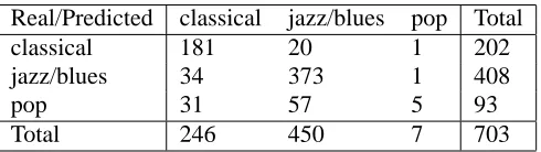
We now simultaneously train our random forest classifier and estimate the best results it could obtain on clean and accurate transcriptions by performing a 5-fold cross-validation on the restricted and re-organised symbolic and synthesised audio dataset we created from the Perez-9-genres Corpus (cf. Section 2.3). The resulting confusion matrices1are given in Table 1 and Table 2. The columns correspond to the predicted music genres and the rows to the actual ones. The average accuracy is 84.8% for symbolic data, and 79.5% for the synthesised audio data, while the baseline classification accuracy is 55.6% and 58%, when attributing the most probable genre to all the songs. The classifiers detects the classical and jazz/blues classes very well but only correctly classifies a small number of pop songs. We believe that this is due to the shortage of pop songs in our training dataset, combined with the unbalanced number of examples in each class: the jazz set is twice as large as the classical set which in turn is twice as large as the pop set. Performance of these classifiers on real audio data will be presented in Section 4.2.
Real/Predicted classical jazz/blues pop Total
classical 218 15 1 234
jazz/blues 9 407 2 418
pop 26 61 13 100
[image:9.595.158.402.343.412.2]Total 253 483 16 752
Table 1.: Confusion matrix (test results of the 5-fold cross-validation) for the harmony-based classifier applied on the classical-jazz/blues-pop restricted and
re-organised version of the Perez-9-genres Corpus (symbolic dataset).
Real/Predicted classical jazz/blues pop Total
classical 181 20 1 202
jazz/blues 34 373 1 408
pop 31 57 5 93
Total 246 450 7 703
Table 2.: Confusion matrix (test results of the 5-fold cross-validation) for the harmony-based classifier applied on the classical-jazz/blues-pop restricted and re-organised version of the Perez-9-genres Corpus (synthesised audio dataset).
1Note that the total numbers of pieces in the tables do not match the total number of pieces in the Perez-9-genres Corpus:
• 5 files in the symbolic dataset have “twins”: i.e. different music pieces with different names which can be represented by the exact same list of chords. These twins are treated as duplicates by TILDE, which automatically removes duplicate files before training, and are thus not counted in the total number of pieces.
• A few files from the Perez-9-genres Corpus were not used in the synthesised audio dataset as they were unusually long
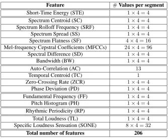
[image:9.595.158.403.492.561.2]Feature #Values per segment
Short-Time Energy (STE) 1×4 = 4
Spectrum Centroid (SC) 1×4 = 4
Spectrum Rolloff Frequency (SRF) 1×4 = 4
Spectrum Spread (SS) 1×4 = 4
Spectrum Flatness (SF) 4×4 = 16
Mel-frequency Cepstral Coefficients (MFCCs) 24×4 = 96
Spectral Difference (SD) 1×4 = 4
Bandwidth (BW) 1×4 = 4
Auto-Correlation (AC) 13
Temporal Centroid (TC) 1
Zero-Crossing Rate (ZCR) 1×4 = 4
Phase Deviation (PD) 1×4 = 4
Fundamental Frequency (FF) 1×4 = 4
Pitch Histogram (PH) 1×4 = 4
Rhythmic Periodicity (RP) 1×4 = 4
Total Loudness (TL) 1×4 = 4
Specific Loudness Sensation (SONE) 8×4 = 32
[image:10.595.112.446.45.323.2]Total number of features 206
Table 3.: Extracted Features
3. Combining Audio and Harmony-based Classifiers
In this section, a standard state-of-the-art classification system employed for genre clas-sification experiments is described. The extracted features are listed in Section 3.1, the feature selection procedure is described in Section 3.2 and finally the fusion procedure is explained and the employed machine learning classifiers are presented in Section 3.3.
3.1 Feature Extraction
In feature extraction, a vector set of numerical representations, that is able to accurately describe aspects of an audio recording, is computed (Tzanetakis and Cook 2002). Ex-tracting features is the first step in pattern recognition systems, since any classifier can be applied afterwards. In most genre classification experiments the extracted features belong to 3 categories: timbre, rhythm, and melody (Scaringella et al. 2006). For our experiments, the feature set proposed in (Benetos and Kotropoulos 2010) was employed, which con-tains timbral descriptors such as energy and spectral features, as well as pitch-based and rhythmic features, thus being able to accurately describe the audio signal. The complete list of extracted features can be found in Table 3.
The feature related to the audio signal energy is the STE. Spectral descriptors of the signal are the SC, SRF, SS, SF, MFCCs, SD (also called spectral flux), and BW. Temporal descriptors include the AC, TC, ZCR, and PD. As far as pitch-based features are con-cerned, the FF feature is computed using maximum likelihood harmonic matching, while the PH describes the amplitude of the maximum peak of the folded histogram (Tzane-takis et al. 2003). The RP feature was proposed in (Pampalk et al. 2004). Finally, the TL feature and the SONE coefficients are perceptual descriptors which are based on auditory modeling.
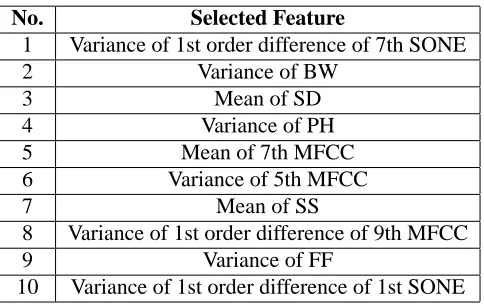
No. Selected Feature
1 Variance of 1st order difference of 7th SONE
2 Variance of BW
3 Mean of SD
4 Variance of PH
5 Mean of 7th MFCC
6 Variance of 5th MFCC
7 Mean of SS
8 Variance of 1st order difference of 9th MFCC
9 Variance of FF
[image:11.595.159.401.46.200.2]10 Variance of 1st order difference of 1st SONE
Table 4.: The subset of 10 selected features.
measures are employed in order to result in a compact representation of the signal char-acteristics. To be specific, their mean and variance are computed along with the mean and variance of the first-order frame-based feature differences over a 1 sec texture window. The same texture window size was used for genre classification experiments in (Tzane-takis and Cook 2002). Afterwards, the computed values are averaged for all the segments of the recording, thus explaining the factor 4 appearing in Table 3. This is applied for all extracted features apart from the AC values and the TC, which are computed for the whole duration of the recording. In addition, it should be noted that for the MFCCs, 24 coefficients are computed over a 10 msec frame (which is a common setting for audio processing applications), while 8 SONE coefficients are computed over the same duration – which is one of the recommended settings in (Pampalk et al. 2004).
3.2 Feature Selection
Although the extracted 206 features are able to capture many aspects of the audio signal, it is advantageous to reduce the number of features through a feature selection procedure in order to remove any feature correlations and to maximize classification accuracy in the presence of relatively few samples (Scaringella et al. 2006). One additional motiva-tion behind feature selecmotiva-tion is the need to avoid the so-called curse of dimensionality phenomenon (Burred and Lerch 2003).
In this work, the selected feature subset is chosen as to maximize the inter/intra class ratio (Fukunaga 1990). The aim of this feature selection mechanism is to select a set of features that maximizes the sample variance between different classes and minimizes the variance for data belonging to the same class, thus leading to classification improvement. The branch-and-bound search strategy is employed for complexity reduction purposes, being also able to provide the optimal feature subset. In the search strategy, a tree-based structure containing the possible feature subsets is traversed using depth-first search with backtracking (van der Hedjen et al. 2004).
For our experiments, several feature subsets were created, containing Θ =
{10,20, . . . ,100}features. In Table 4, the subset for 10 selected features is listed, where
it can be seen that the MFCCs and the SONE coefficients appear to be discriminative features.
3.3 Classification System
Audio files
Chords
Low-level signal-based features Harmony
feature
Genre classification Symbolic
database
[image:12.595.145.414.53.297.2]Harmony rules
Figure 2.: Block diagram of the genre classifier
3.1 and 3.2 with the output of the harmony-based classifier described in Section 2. Con-sidering the extracted feature vector for a single recording asv(with lengthΘ) and the
respective output of the harmony-based classifier asr= 1, . . . , C, whereCis the number of genre classes, a combined feature vector is created in the form ofv′ = [vr]. Thus, the
output of the harmony-based classifier is treated as an additional feature used, along with the extracted and selected audio features, as an input to the learning phase of the overall genre classifier.
Two machine learning classifiers were employed for the genre classification experi-ments, namely multilayer perceptrons (MLPs) and support vector machines (SVMs). For the MLPs, a 3-layered perceptron with the logistic activation function was utilized, while training was performed with the back-propagation algorithm for learning rate equal to 0.3, 500 training epochs, and momentum equal to 0.1. A multi-class SVM classifier with a 2nd order polynomial kernel with unit bias/offset was also used (Sch¨olkopf et al. 1999). The experiments with the aforementioned classifiers were conducted on the training matrix
V′ = [v′
1v′2 · · · vM′ ], whereM is the number of training samples.
4. Experiments
4.1 Datasets
Two commonly used datasets in the literature were employed for genre classification ex-periments. Firstly, the GTZAN database was used, which contains 1000 audio recordings distributed across 10 music genres, with 100 recordings collected for each genre (Tzane-takis and Cook 2002). From the 10 genre classes, 3 were selected for the experiments, namely the classical, jazz, and pop classes. All recordings are mono channel, are sampled at 22.05 kHz rate and have a duration of approximately 30 sec.
26, and the pop/rock class 102. The duration of the recordings is not constant, ranging from 19 seconds to 14 minutes. The recordings were sampled at 22kHz rate and were converted from stereo to mono.
4.2 Results
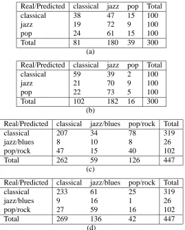
First the harmony-based classifier (trained on both the re-organised symbolic and synthe-sised audio Perez-9-genres datasets) was tested on these two audio datasets. The results are shown in Table 5. For the GTZAN dataset, the classification accuracy using the harmony-based classifier is 41.67% (symbolic training) and 44.67% (synthesised audio training), while for the ISMIR04 dataset it is 57.49% (symbolic training) and 59.28% (synthesised audio training). Even though the classifier trained on synthesised audio data obtained worse results than the one trained on symbolic data when performing cross-validation on the Perez-9-genres datasets, the opposite trend is observed here when tested on the two real audio datasets. We believe the symbolic model does not perform as well on audio data because it assumes that the chord progressions are perfectly transcribed, which is not the case. The synthesised audio model on the other hand does account for this noise in transcription (and includes it in its grammar rules). Given these results we will use the classifier trained on synthesised audio data in the experiments merging the harmony-based and the audio feature based classifiers.
Real/Predicted classical jazz pop Total
classical 38 47 15 100
jazz 19 72 9 100
pop 24 61 15 100
Total 81 180 39 300
(a)
Real/Predicted classical jazz pop Total
classical 59 39 2 100
jazz 21 70 9 100
pop 22 73 5 100
Total 102 182 16 300
(b)
Real/Predicted classical jazz/blues pop/rock Total
classical 207 34 78 319
jazz/blues 8 10 8 26
pop/rock 47 15 40 102
Total 262 59 126 447
(c)
Real/Predicted classical jazz/blues pop/rock Total
classical 233 61 25 319
jazz/blues 9 16 1 26
pop/rock 27 59 16 102
Total 269 136 42 447
[image:13.595.146.415.321.655.2](d)
Table 5.: Confusion matrices for the harmony-based classifier trained on: (a) symbolic data and applied on the GTZAN dataset, (b) synthesised audio data and applied on the GTZAN dataset, (c) symbolic data and applied on the ISMIR04 dataset, (d) synthesised
Feature Subset Size
C
la
ss
ific
at
io
n
A
cc
u
ra
cy
%
MLP-H SVM-H MLP+H SVM+H
10 20 30 40 50 60 70 80 90 100 Full
[image:14.595.109.444.53.313.2]45 50 55 60 65 70 75 80 85 90 95 100
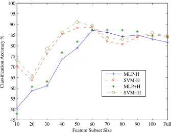
Figure 3.: Classification accuracy for the GTZAN dataset using various feature subsets.
Then experiments using the SVM and MLP classifiers with 5x5-fold cross-validation were performed using the original extracted audio feature vectorv which does not
in-clude the output of the harmony-based classifier. First these classifiers were tested on the synthesised Perez-9-genres Corpus which is described in Section 2.3. The full set of 206 audio features was employed for classification. For the SVM, classification accuracy is 95.56%, while for the MLP classifier, the classification accuracy is 95.67%. While clas-sification performance appears to be very high compared to the harmony-based classifier for the same data, it should be stressed that the Perez-9-genres dataset consists of synthe-sised MIDI files, making the dataset unsuitable for audio processing-based experiments. This happens because these files use different sets of synthesised instruments for each of the 3 genres, which produce unrealistic results when a timbral feature-based classifier is employed.
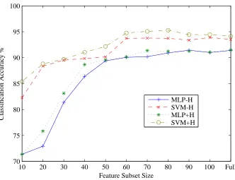
Finally, experiments comparing results of the SVM and MLP classifiers with and with-out the with-output of the harmony-based classifier (trained on synthesised audio data) were performed with the various feature subsets on the SVM and MLP classifiers using 5x5-fold cross-validation. The average accuracy achieved by the classifiers using 5x5-5x5-fold cross-validation for the various feature subset sizes using the GTZAN dataset is shown in Figure 3, while the average accuracy for the ISMIR04 dataset is shown in Figure 4. In Table 6 the best accuracy achieved for the various feature subsets and classifiers is pre-sented. The SVM-H and MLP-H classifiers stand for the standard feature setv(without
harmony), while the SVM+H and MLP+H classifiers stand for the feature setv′ (with harmony).
Feature Subset Size
C
la
ss
ific
at
io
n
A
cc
u
ra
cy
%
MLP-H SVM-H MLP+H SVM+H
10 20 30 40 50 60 70 80 90 100 Full
[image:15.595.111.443.51.306.2]70 75 80 85 90 95 100
Figure 4.: Classification accuracy for the ISMIR04 dataset using various feature subsets.
Classifier GTZAN Dataset ISMIR04 Dataset
SVM-H 88.66% (60 Features) 93.77% (70 Features)
SVM+H 91.13% (50 Features) 95.30% (80 Features)
MLP-H 87.19% (60 Features) 91.45% (90 Features)
MLP+H 87.53% (60 Features) 91.49% (Full Feature Set)
Table 6.: Best mean accuracy achieved by the various classifiers for the GTZAN and ISMIR04 datasets using 5x5-fold cross-validation.
rates over the SVM-H and MLP-H classifiers, respectively. There are however some cases where the classification rate is identical, for example for the MLP classifiers using the 60 features subset for the ISMIR04 dataset. The fact that the ISMIR04 rates are higher than the GTZAN rates can be attributed to the class distribution.
In order to compare the performance of the employed feature set with other feature sets found in the literature, the extracted features from the MARSYAS (Tzanetakis 2007) toolbox were employed, which contain the mean values of the spectral centroid, spectral rolloff, spectral flux, and the mean values of 30 MFCCs for a 1sec texture window. Results on genre classification using the MARSYAS feature set with 5x5-fold cross-validation on both datasets and using the same classifiers (SVM, MLP) and their respective settings can be seen in Table 7, where it can be seen that for the MLP classifier, the classification accuracy between the MARSYAS feature set and the employed feature set is roughly the same for both datasets. However, when the SVM classifier is used, the employed feature set outperforms the MARSYAS features by at least 3% for the GTZAN case and 4% for the ISMIR04 set. It should be noted however that no feature selection took place for the MARSYAS features.
Classifier GTZAN Dataset ISMIR04 Dataset
SVM 85.66% 91.51%
[image:16.595.160.402.48.90.2]MLP 85.00% 91.96%
Table 7.: Mean accuracy achieved by the various classifiers for the GTZAN and ISMIR04 datasets, using the MARSYAS feature set and 5x5-fold cross-validation.
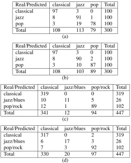
misclassifications occur for the pop class, in both cases. However, the SVM+H algorithm rectifies some misclassifications of the pop class compared to the SVM-H classifier. For the ISMIR04 dataset, most misclassifications occur for the jazz/blues class for both clas-sifiers. Even for the SVM+H classifier, when taking normalized rates, the jazz/blues class suffers the most, having only 63.58% correct classification rate. It should be noted though that the SVM+H classifier has 6 more jazz/blues samples correctly classified compared to the SVM-H one. The classical class on the other hand, seems largely unaffected by misclassifications.
Real/Predicted classical jazz pop Total
classical 97 3 0 100
jazz 8 91 1 100
pop 3 19 78 100
Total 108 113 79 300
(a)
Real/Predicted classical jazz pop Total
classical 97 3 0 100
jazz 8 90 2 100
pop 3 10 87 100
Total 108 103 89 300
(b)
Real/Predicted classical jazz/blues pop/rock Total
classical 319 0 0 319
jazz/blues 10 11 5 26
pop/rock 12 1 89 102
Total 341 12 94 447
(c)
Real/Predicted classical jazz/blues pop/rock Total
classical 317 0 2 319
jazz/blues 6 17 3 26
pop/rock 7 3 92 102
Total 330 20 97 447
(d)
Table 8.: Confusion matrices for one 5-fold cross validation run of: (a) the SVM-H classifier applied on the GTZAN dataset using the 60 selected features set, (b) the SVM+H classifier applied on the GTZAN dataset using the 50 selected features set, (c) the SVM-H classifier applied on the ISMIR04 dataset using the 70 selected features set, (d) the SVM+H classifier applied on the ISMIR04 dataset using the 80 selected features
set.
[image:16.595.144.415.258.595.2]was employed, which is applied to 2x2 contingency tables for a single classifier run. We consider the cases exhibiting the highest classification rates, as shown in Table 6. For the GTZAN dataset, the SVM-H classifier using the 60 features set is compared against the SVM+H classifier using the 50 features set. For the ISMIR04 dataset, the SVM-H classifier using 70 features is compared against the SVM+H classifier using 80 features. The contingency tables for the GTZAN and ISMIR04 datasets are respectively:
· 264 10
2 24 ¸
and ·
416 10 3 18 ¸
(1)
The binomial distribution is used to obtain the McNemar test statistic, where for both cases the null hypothesis (the difference between the two classifiers is insignificant) is rejected with 95% confidence.
4.3 Discussion
This improvement of the classification results might come as a surprise when one consid-ers that the harmony-based classifier by itself does not perform sufficiently well on audio data. Indeed on the ISMIR04 dataset its accuracy is lower than the baseline (59.28% vs. 71.36%). However, harmony is only one dimension of music which despite being rele-vant for genre identification can not capture by itself all genres’ specificities. The authors believe that the classification improvement lies in the fact that it covers an aspect of the audio-signal (or rather of its musical properties) that the other (low-level) features of the classifier do not capture.
In order to justify that the combination of several features improves classification ac-curacy even when they are lower than the baseline, the mean of the 5th MFCC was em-ployed as an example feature. 5-fold cross-validation experiments were performed on the GTZAN and ISMIR04 datasets based on this single feature using SVMs. Results indicated that classification accuracy for the GTZAN dataset was 31.33%, while for the ISMIR04 dataset it was 71.36%, both of which are below the baseline. However the feature, being one of the selected ones, when combined with several other features manages to report a high classification rate as shown in Section 4.2. Thus, the inclusion of the output of the harmony-based classifier, while being lower than the baseline by itself, still manages to provide improved results when combined with several other descriptors. In addition, in order to compare the addition of the harmony-derived classification to the feature set with an additional feature, the Total Loudness (TL) was added into the SVM-H classifier using the 70 features subset (TL is not included in the set). Using the GTZAN dataset for ex-periments, classification accuracy for the 70 features subset is 82%, while adding the TL feature it increased by 0.66%, where the performance improvement is lower compared to the harmony-based classifier addition (which was 1.66%).
5. Conclusions
In the future, the combination of the low-level classifier with the harmony-based classifier can be expanded, where multiple features stemming from chord transitions can be com-bined with the low-level feature set in order to boost performance. In addition, the chord transition rules can be modeled to describe more genres, leading to experiments con-taining more elaborate genre hierarchies. This would allow to test how well our method scales.
and built using the Inductive Logic Programming algorithm TILDE. Three-class genre classification experiments were performed on two commonly used datasets, where an im-provement was reported for both cases when the harmony-based classifier was combined with a low-level feature set using support vector machines and multilayer perceptrons. The combination of these low-level features with the harmony-based classifier produces improved results despite the fact that the classification rate of the harmony-based classi-fier is not sufficiently high by itself. For both datasets when the SVM classiclassi-fier was used, the improvement over the standard classifier was found to be statistically significant when the highest classification rate is considered. All in all, it was shown that the combination of high-level harmony features with low-level features can lead to genre classification accuracy improvements and is a promising direction for genre classification research.
6. Acknowledgements
This work was done while the third author was a Research Student at Queen Mary, Univer-sity of London. This work is supported by the EPSRC project OMRAS2 (EP/E017614/1) and Emmanouil Benetos is supported by a Westfield Trust PhD Studentship (Queen Mary, University of London). The authors would like to thank the Pattern Recognition and Arti-ficial Intelligence Group of the University of Alicante for providing the symbolic training dataset.
References
Anglade, A., Ramirez, R., and Dixon, S. (2009a). First-order logic classification models of musical genres based on harmony. In Proceedings of the 6th Sound and Music Computing Conference (SMC 2009), pages 309–314, Porto, Portugal.
Anglade, A., Ramirez, R., and Dixon, S. (2009b). Genre classification using harmony rules induced from automatic chord transcriptions. In Proceedings of the 10th International Conference on Music Information Retrieval (ISMIR 2009), pages 669–674, Kobe, Japan.
Assche, A. V., Vens, C., Blockeel, H., and Dˇzeroski, S. (2006). First order random forests: Learning relational classifiers with complex aggregates. Machine Learning, 64:149–182.
Aucouturier, J.-J. and Pachet, F. (2004). Improving timbre similarity: How high is the sky? Journal of Negative Results in Speech and Audio Science, 1(1).
Aucouturier, J.-J. and Pachet, F. (2008). A scale-free distribution of false positives for a large class of audio similarity measures. Pattern recognition, 41(1):272–284.
Benetos, E. and Kotropoulos, C. (2010). Non-negative tensor factorization applied to music genre classification. IEEE Trans. Audio, Speech, and Language Processing, 18(8):1955–1967.
Blockeel, H. and De Raedt, L. (1998). Top down induction of first-order logical decision trees. Artificial Intelligence, 101(1-2):285–297.
Breiman, L. (2001). Random forests. Machine Learning, 45:5–32.
Burred, J. J. and Lerch, A. (2003). A hierarchical approach to automatic musical genre classification. In Proceedings of the 6th International Conference on Digital Audio Effects (DAFx 2003), pages 8–11, Kobe, Japan.
Cataltepe, Z., Yaslan, Y., and Sonmez, A. (2007). Music genre classification using MIDI and audio features. EURASIP Journal on Advances in Signal Processing.
Chen, L., Wright, P., and Nejdl, W. (2009). Improving music genre classification using collaborative tagging data. In Proceedings of the 2nd ACM International Conference on Web Search and Data Mining (WSDM ’09), pages 84–93, Barcelona, Spain.
Davies, M. E. P., Plumbley, M. D., and Eck, D. (2009). Towards a musical beat emphasis function. In Proceedings of the IEEE Workshop on Applications of Signal Processing to Audio and Acoustics (WASPAA 2009), pages 61–64, New Paltz, NY.
Downie, J. S., Byrd, D., and Crawford, T. (2009). Ten years of ISMIR: reflections on challenges and opportunities. In Proceedings of the 10th International Conference on Music Information Retrieval (ISMIR 2009), pages 13–18, Kobe, Japan.
Fukunaga, K. (1990). Introduction to Statistical Pattern Recognition. Academic Press Inc., San Diego, CA.
Harte, C. and Sandler, M. Automatic chord identification using a quantised chromagram. In Proceedings of 118th Conven-tion, Barcelona, Spain. Audio Engineering Society.
ISMIR (2004). ISMIR audio description contest. http://ismir2004.ismir.net/ISMIR Contest.html. Lawson, C. L. and Hanson, R. J. (1974). Solving Least Squares Problems, chapter 23. Prentice-Hall.
Lee, J. H., Jones, M. C., and Downie, J. S. (2009). An analysis of ISMIR proceedings: patterns of authorship, topic and citation. In Proceedings of the 10th International Conference on Music Information Retrieval (ISMIR 2009), pages 57–62, Kobe, Japan.
Lidy, T., Rauber, A., Pertusa, A., and I˜nesta, J. M. (2007). Improving genre classification by combination of audio and sym-bolic descriptors using a transcription system. In Proceedings of the 8th International Conference on Music Information Retrieval (ISMIR 2007), pages 61–66, Vienna, Austria.
Mauch, M. (2010). Automatic Chord Transcription from Audio Using Computational Models of Musical Context. PhD thesis, Queen Mary University of London.
Mauch, M., Dixon, S., Harte, C., Casey, M., and Fields, B. (2007). Discovering chord idioms through beatles and real book songs. In Proceedings of the 8th International Conference on Music Information Retrieval (ISMIR 2007), pages 255–258, Vienna, Austria.
McKay, C. and Fujinaga, I. (2006). Musical genre classification: is it worth pursuing and how can it be improved? In Pro-ceedings of the 7th International Conference on Music Information Retrieval (ISMIR 2006), pages 101–106, Victoria, Canada.
McKay, C. and Fujinaga, I. (2008). Combining features extracted from audio, symbolic and cultural sources. In Proceedings of the 9th International Conference on Music Information Retrieval (ISMIR 2008), pages 597–602, Philadelphia, PA. McNemar, Q. (1947). Note on the sampling error of the difference between correlated proportions or percentages.
Psy-chometrika, 12(2):153–157.
Meng, A., Ahrendt, P., and Larsen, J. (2005). Improving music genre classification by short-time feature integration. In Proceedings of the 2005 IEEE International Conference on Acoustics, Speech, and Signal Processing (ICASSP 2005), volume 5, pages v/497 – v/500, Philadelphia, PA.
Muggleton, S. (1991). Inductive logic programming. New Generation Computing, 8(4):295–318.
Muggleton, S. H., Bryant, C. H., Srinivasan, A., Whittaker, A., Topp, S., and Rawlings, C. (2001). Are grammatical representations useful for learning from biological sequence data? - a case study. Journal of Computational Biology, 8(5):493–522.
Neumayer, R. and Rauber, A. (2007). Integration of text and audio features for genre classification in music information retrieval. In Proceedings of the 29th European Conference on Information Retrieval (ECIR 2007), pages 724–727, Rome, Italy.
Pampalk, E., Dixon, S., and Widmer, G. (2004). Exploring music collections by browsing different views. Computer Music Journal, 28(2):49–62.
P´erez-Sancho, C. (2009). Stochastic language models for music information retrieval. PhD thesis, Universidad de Alicante. P´erez-Sancho, C., Rizo, D., I˜nesta, J. M., Ponce de Le´on, P. J., Kersten, S., and Ramirez, R. (2010). Genre classification of
music by tonal harmony. Intelligent Data Analysis. in press.
P´erez-Sancho, C., Rizo, D., and Inesta, J. M. (2009). Genre classification using chords and stochastic language models. Connection Science, 21(2 & 3):145–159.
Piston, W. (1987). Harmony. Norton, W. W. & Company, Inc., 5th edition.
Quinlan, J. R. (1993). C4.5: programs for machine learning. Morgan Kaufmann Publishers Inc.
Rabiner, L. R. (1989). A tutorial on hidden Markov models and selected applications in speech recognition. Proceedings of the IEEE, 77(2):257–286.
Scaringella, N., Zoia, G., and Mlynek, D. (2006). Automatic genre classification of music content. IEEE Signal Processing Magazine, 23(2):133–141.
Sch¨olkopf, B., Burges, C. J. C., and Smola, A. J. (1999). Advances in Kernel Methods: Support Vector Learning. Cambridge MA, USA: MIT Press.
Shan, M.-K., Kuo, F.-F., and Chen, M.-F. (2002). Music style mining and classification by melody. In Proceedings of 2002 IEEE International Conference on Multimedia and Expo (ICME’02), volume 1, pages 97–100.
Tzanetakis, G. (2007). Marsyas: a case study in implementing music information retrieval systems. In Shen, J., Shepherd, J., Cui, B., and Liu, L., editors, Intelligent Music Information Systems: Tools and Methodologies, pages 31–49. Idea Group Reference.
Tzanetakis, G. and Cook, P. (2002). Musical genre classification of audio signals. IEEE Transactions on Audio, Speech, and Language Processing, 10(5):293–302.
Tzanetakis, G., Ermolinskyi, A., and Cook, P. (2003). Pitch histograms in audio and symbolic music information retrieval. Journal of New Music Research, 32(2):143–152.
van der Hedjen, F., Duin, R. P. W., de Ridder, D., and Tax, D. M. J. (2004). Classification, Parameter Estimation and State Estimation. London UK: Wiley.