Delay models for static and adaptive persistent resource allocations in wireless systems

(1)

Delay Models for Static and Adaptive Persistent

Resource Allocations in Wireless Systems

Jason Brown, Nusrat Afrin and Jamil Y Khan

School of Electrical Engineering and Computer Science

The University of Newcastle Callaghan, NSW 2308, AUSTRALIA

Email: [email protected], [email protected], [email protected]

Abstract— A variety of scheduling strategies can be employed

in wireless systems to satisfy different system objectives and to cater for different traffic types. Static persistent resource allocations can be employed to transfer small M2M data packets efficiently compared to dynamic packet-by-packet scheduling, even when the M2M traffic model is non-deterministic. Recently adaptive persistent allocations have been proposed in which the volume of allocated resources can change in sympathy with the instantaneous queue size at the M2M device and without expensive signaling on control channels. This increases the efficiency of resource usage at the expense of a (typically small) increased packet delay. In this paper, we derive a statistical model for the device queue size and packet delay in static and adaptive persistent allocations which can be used for any arrival process (i.e., Poisson or otherwise). The primary motivation is to assist with dimensioning of persistent allocations given a set of QoS requirements (such as a prescribed delay budget). We validate the statistical model via comparison with queue size and delay statistics obtained from a discrete event simulation of a persistent allocation system. The validation is performed for both exponential and gamma distributed packet inter-arrivals to demonstrate the model generality.

Index Terms— M2M, persistent allocation, wireless system,

delay model

I.INTRODUCTION

Machine-to-Machine (M2M) applications are widespread in a wide variety of markets including automotive, healthcare and utilities. For example, a Smart Grid typically supports multiple user and network oriented M2M applications such as Advanced Metering Infrastructure (AMI), automated Demand Response (DR), Fault Detection, Isolation and Restoration (FDIR) and Wide Area Measurement System (WAMS) [1]. These applications can have diverse Quality-of-Service (QoS) requirements; for example, AMI is typically not particularly delay sensitive whereas FDIR and WAMS are. However, there are also some commonalities between many M2M applications [2]: a relatively large number of devices, relatively small packet sizes, uplink biased traffic and low or no mobility compared to Human-to-Human (H2H) and Human-to-Machine (H2M) communication.

There has been considerable interest in employing wide area wireless broadband systems such as 3GPP Long Term Evolution (LTE) and IEEE 802.16/Worldwide Interoperability for Microwave Access (WiMAX) networks for M2M

applications due to their ubiquity, high economies of scale, high spectral efficiency, relatively low latency, robust network security and support for a wide variety of frequency bands and bandwidths compared to previous cellular standards [3-6]. However, these standards were originally designed primarily for H2H and H2M communications (even though they are capable of supporting any IP based application) and the standards bodies have only recently started development of enhancements to efficiently support typical M2M applications [7-8]. One major concern has been the likelihood of an overloaded random access channel caused by a large number of M2M devices located in each cell. Much research has been dedicated to this specific topic and many different solutions proposed [9][10]. This paper addresses a different issue which occurs when M2M devices have successfully completed the random access procedure in order to send uplink data.

(2)

[image:2.595.45.289.120.293.2]

the M2M application is delay sensitive, there is clearly a need to establish the distribution of packet delays using this scheme.

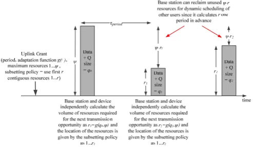
Fig. 1: Comparison of Resource Allocation Schemes (from the Perspective of One Device)

We note that a (static) persistent uplink resource allocation tends to be most appropriate for event driven devices which send a stream of packets with an arbitrary arrival process once some event is detected. For example, a sensor may not send any packets for a considerable duration, but once it detects a specific event, it may send packets to communicate the ongoing situation for an extended duration. Concrete M2M applications listed in [17] that may be suitable for a persistent resource allocation because they involve an ongoing stream of packets include Wide Area Measurement System (WAMS) for the smart grid, oil/gas pipeline monitoring, a healthcare gateway and video surveillance at traffic lights. Some of these applications involve individual devices feeding in to an M2M gateway over a personal or local area network, and the gateway aggregating/relaying traffic over a wide area network. In these scenarios, the M2M gateway is usually a good candidate for a persistent resource allocation because it sends an aggregated stream of packets and the aggregation is performed over a duration that fits well with the concept of a periodic allocation of resources. Dynamic packet-by-packet scheduling may still be more appropriate than the use of a persistent uplink resource allocation for some types of M2M devices, particularly those that send a small amount of data on an infrequent basis.

An extension of static persistent uplink resource allocation scheme is adaptive persistent uplink resource allocation as proposed in [18] for the specific case of an LTE network. In this scheme, the volume of uplink resources assigned to a device can vary from one transmission opportunity to the next as illustrated in Fig. 1(c) based upon common knowledge at the device and base station about the device queue size. Both the device and base station use the most recent queue size data available as input to a pre-agreed adaptation function to calculate the volume of uplink resources required for the next transmission opportunity (up to some maximum negotiated when the persistent allocation is initiated) without any need to signal updated uplink grants on the downlink control channel.

This is clearly more efficient than static persistent uplink resource allocation for non-deterministic traffic sources (provided the adaptation function is chosen rationally) since the device consumes only the necessary uplink resources as dictated by its prevailing queue size. The uplink resources saved using this method can then be used by the base station for dynamic packet-by-packet scheduling of other network users. There does need to be a common understanding between the device and base station about which subset of nominally assigned resources are used when less than the maximum is required, and the details of this subsetting arrangement can either be known implicitly by both parties or communicated explicitly in the initial setup message for the persistent resource allocation sent by the base station. The scheme is illustrated in more detail in Fig. 2 for an example subsetting policy in which assigned resources are always contiguous.

Fig. 2: Adaptive Persistent Uplink Resource Allocation Details

The key aspect of the adaptive persistent resource allocation scheme is that the device and base station are independently calculating the volume (using the adaptation function ∙) and specific subset (in this example 1, 2. . ) of the resources (using the subsetting policy) which are required for each and every transmission opportunity one period in advance based upon the parameters in the initial uplink grant. There are two important implications of this:

i. Since the device and base station independently calculate which specific resources to use for each and every transmission opportunity, there is no need for the base station to explicitly signal the resources to be used on the downlink control channel on an ongoing basis.

[image:2.595.306.553.269.412.2]

(3)

In adaptive persistent uplink resource allocation, the device queue size information is typically communicated from the device to the base station during each transmission opportunity and then used by both entities to calculate the volume of uplink resources required for the next transmission opportunity. For example, in LTE, the Buffer Status Report (BSR) [16] provides this queue size information. The device may of course generate more packets between the two transmission opportunities; although the device clearly knows at all times its instantaneous queue size, the base station only knows the queue size at the previous transmission opportunity. Therefore both entities must use the base station knowledge as input to the adaptation function when calculating the volume of uplink resources required for the next transmission opportunity in order to arrive at a common result. The adaptation function may attempt to predict the number of packets generated between transmission opportunities based upon known or estimated traffic parameters in order to better match the calculated volume of uplink resources with the actual instantaneous queue size at the time of the next transmission opportunity. Even so, in general, there will be occasions when the calculated volume of uplink resources is less than the maximum permissible for the persistent allocation, but insufficient to serve the full device queue. Therefore the adaptation comes at a cost in terms of increased delay relative to a static persistent uplink resource allocation because a static allocation could have served more packets during the transmission opportunity in this scenario. The relative distribution of packet delays for static and adaptive persistent uplink resource allocations is therefore of great interest when the M2M application is delay sensitive.

While one benefit of the adaptive persistent uplink resource allocation scheme is that it can reduce resource utilisation/wastage at the expense of packet delay in a stationary environment, a second and possibly more significant advantage is that it can automatically adjust the resource utilisation within the lifetime of a persistent allocation in sympathy with dynamic changes to the arrival process of packets at the device without additional signalling on the downlink control channel. For example, if there is a temporary cessation to packet generation at the device, the adaptive persistent uplink resource allocation scheme can automatically reduce the assigned resources to the minimal possible to preserve the persistent allocation, and then ramp up again once the device begins to generate more packets. This is not possible with the static persistent uplink resource allocation scheme; first the change in arrival process must be detected at the base station, then a persistent allocation modification or teardown message must be sent on the downlink control channel to the device.

With reference to Fig. 1(a)-(c), if we assume that queue size overhead information is communicated during each transmission opportunity of a persistent allocation, it is possible that the total overhead in doing so may be more or less than the corresponding overhead that would have occurred if dynamic scheduling had been used instead. This depends upon the nature of the dynamic scheduling algorithm in use, and in particular whether the scheduler tends to provide uplink grants

for small amounts of data frequently or large amounts of data infrequently. This is an important topic as it affects the efficiency of the system as a whole; however we do not discuss it further as the objective of this paper is to provide a performance model of individual static and adaptive persistent resource allocations.

In order to quantify the delay in the static persistent uplink resource allocation scheme, we note that from the perspective of the device, the persistent allocation is similar to an assignment in a TDMA system in that a fixed amount of resources are assumed by both ends of the wireless link on a periodic basis. Queuing models for TDMA systems have been studied in depth in different contexts in the literature [19-24]. For example, in [19-20], one timeslot per TDMA frame is allocated to a device and one packet can be transferred per timeslot. In [21-23], multiple contiguous timeslots per TDMA frame can be allocated to a device to allow serial transfer of multiple packets. However, the static persistent uplink resource allocation scheme described in this paper is subtly different because the assumption is that multiple packets can be transmitted simultaneously (i.e., in parallel) during a transmission opportunity. This is sometimes referred to as bulk service [25] in queueing theory and clearly impacts the queue size and delay distributions. The bulk service assumption is consistent with the OFDM/OFDMA multiple access employed in LTE and 802.16 networks in which different packets are assigned to different subcarrier blocks, although we do not assume any specific features of OFDM/OFDMA or LTE/802.16 in our analysis.

In this paper, we derive the device queue size probability mass function (pmf) and delay probability density function (pdf) for the static and adaptive persistent uplink resource allocation schemes for a general/arbitrary packet arrival process. The device is assumed to have a single queue of unlimited capacity in which packets are served with a First Come First Served (FCFS) queue discipline. This is typical of many M2M devices which have a single function and therefore do not need to support internal prioritisation of packets. We assume that the device has a fixed geographical location such that the channel quality is time invariant and therefore link adaptation is unnecessary. In addition we assume a constant packet size which is typical of many M2M applications [26-28], particularly those related to monitoring such as Wireless Sensor Networks (WSNs). This implies that for a given amount of allocated resources, the volume of data that can be served in terms of the number of packets is time invariant. The primary motivation in deriving the queue size and delay distributions is to allow the parameters of a persistent resource allocation, in particular the transmission opportunity period and the (maximum) amount of allocated resources per transmission opportunity, to be easily and accurately determined to allow a delay sensitive M2M application to satisfy a specific packet delay budget criterion.

(4)

requirements, source traffic characteristics, charging policies and instantaneous carried traffic volume. It may involve online or offline input from the end user particularly if the different schemes are charged differently. We do not address policy or system related issues in this paper, but instead concentrate on objective performance characterisation of static and adaptive persistent resource allocations.

The paper is organised as follows. In Section II, we present the system model for the static and adaptive persistent uplink resource allocation schemes. We use this model in Section III to derive the queue size and delay distributions. We also derive the expected service capacity for the adaptive case. In Section IV, we validate the mathematical models by comparison with the queue size and delay statistics generated by a discrete event simulation model of the persistent uplink resource allocation schemes. The validation involves consideration of packet inter-arrivals which are distributed according to an exponential distribution and a gamma distribution in order to demonstrate the generic nature of the models. Finally, in Section V, we draw conclusions.

II.SYSTEM MODEL

A.Static Allocation

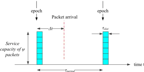
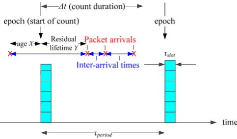
Fig. 3 illustrates the system model and parameters for static persistent uplink resource allocations as discussed in Section I. A device is provided with persistent allocation epochs with service time and period such that up to packets pending in the device queue can be sent each epoch. We consider the packets which are to be sent as being removed from the queue at a single point in time (i.e., the epoch) which corresponds to the start of the service time. will usually be an integer multiple of in practice, although we do not make this assumption in any of the following analysis. , and are parameters of the system and/or the specific persistent allocation and are assumed fixed for the duration of the allocation.

When a new packet is generated by the device at a time Δ

after the previous persistent allocation epoch, there is a random duration Δ until the next epoch, which is the earliest point in time that the packet can be sent or served. is a continuous uniform random variable such that

[image:4.595.44.287.582.704.2]

~ 0, .

Fig. 3: System Model for Static Persistent Allocations

Let the queue size at the time the packet is generated be . The packet is then the 1 packet in the queue and must wait 1 ⁄ persistent allocation epochs to be sent. The duration between the next persistent allocation epoch and the epoch in which the packet is sent is 1 ⁄

1 ⁄ where we use the identity

1 ⁄ 1 / .

The delay for a packet to be sent is therefore:

1 Δ (1)

Since and are random variables, so is . In order to derive the probability distribution of , the distribution of first needs to be determined. We note that is a function of time; as we move from one persistent allocation epoch (Δ=0) to the next (Δ = ), the expected queue size increases linearly (assuming the rate parameter is constant) because new packets are being generated, but existing packets at the head of the queue are not being serviced. Then as we reach the next persistent allocation epoch, up to packets can be serviced in bulk simultaneously such that drops.

A stable system for which the number of packets in the queue does not increase in an unbounded manner requires the expected number of packet arrivals during , , to be less than the maximum number of packet departures during the same period. Alternatively, we may say that the load

⁄ 1 for a stable system. B.Adaptive Allocation

The same system model applies for the adaptive persistent uplink resource allocations discussed in Section I with the exception that the number of packets that can be sent during each epoch can vary from one epoch to the next. We represent the instantaneous service capacity at an epoch as a random variable . We let , where , is a generic adaptation function of the size of the remaining queue immediately after the previous epoch and the maximum service capacity . The only assumption we make about , is that it provides a rational mapping in the sense that:

, ∈

1 ,

, ,

(2)

This means that the instantaneous service capacity is greater than or equal to the size of the remaining queue immediately after the previous epoch unless the maximum service capacity would be exceeded as a result, in which case the maximum service capacity is employed. These

τperiod

τslot Δt

Packet arrival

time t

epoch epoch

Service capacity of ψ

(5)

conditions minimize the possibility that the queue grows without bound.

, is not allowed to return a zero value when 0

because it must always be possible for a device to communicate its remaining queue size to the base station as part of the next persistent allocation transmission even if there are no application packets pending in the queue at the time of this transmission. We assume that the remaining queue size is not communicated via its own packet; rather it is piggybacked in the header of a packet serviced from the device queue, or else piggybacked in the header of a dummy packet if the device queue is empty.

With regard to the delay for a packet to be sent in the adaptive case, we note here that is a random variable which is a function of the queue size at the time the packet arrives and the adaptation function , . This is discussed in greater detail in Section III.

III.ANALYSIS

A.Queue Size Distribution (Static Allocation)

In this section, we first derive the probability mass function (pmf) of the queue size immediately after packets have been removed or serviced from the queue for a static persistent resource allocation. This can be used as the basis for deriving the pmf of at an arbitrary point in time by considering the statistics of packet arrivals since the last service time.

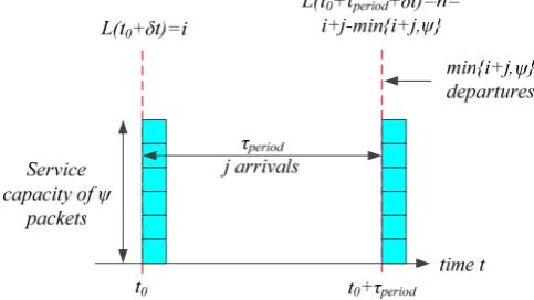
We assume packets are removed from the queue for service at single points in time, the persistent allocation epochs, which occur periodically at times , … etc. as illustrated in Fig. 4. We define a time immediately after the first epoch at which . If the number of packet arrivals between the first and second epochs is , immediately prior to the second epoch. Since a maximum of packets can be removed from the queue and sent at the second epoch, then at time immediately after the second epoch,

0 if and if .

Alternatively, this can be expressed as

[image:5.595.43.285.533.669.2]

, .

Fig. 4: Background to the Analysis of Queue Size L Immediately After a Static Persistent Allocation Epoch

To derive the limiting probability that at time immediately after the second epoch as → 0, which we denote as lim

→ . we consider

the various combinations of events (i.e., packet arrivals and departures) that can occur starting one period earlier at time

when .

There are two individual components of lim →

to consider defined by different relationships between , and :

i. . In this case, 0 and 0 by

definition. The complete queue of size that exists immediately prior to the second epoch can be serviced

such that 0 at time

immediately after the epoch. Therefore lim →

is given by considering all possible values of and that satisfy the above constraints as follows:

lim

→

lim

→ (3)

where:

 Δ is the probability of packets arriving during the interval Δ. For example, for Poisson arrivals with rate parameter , Δ

! .

ii. . In this case, the queue of size that exists immediately prior to the second epoch can only be partially serviced such that 0 at time

immediately after the epoch. Considering the equation leads to the

constraints 0 and . Therefore

→ is given by considering all

possible values of and that satisfy the above constraints as follows:

lim

→

lim

→

∀ 1

(4)

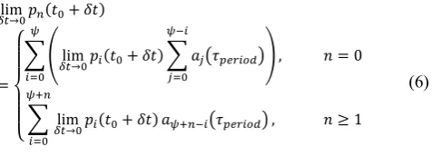
For a stable system as described in Section II such that , or alternatively ⁄ 1:

lim

→ lim→ ∀ ₍₅₎

(6)

lim

→

lim

→ , 0

lim

→ , 1

(6)

Eq. (6) forms a system of homogeneous linear equations in the variables lim

→ which collectively represent

the pmf of the queue size immediately after a persistent allocation epoch. The equation coefficients are derived from the count model which in theory can be calculated according to any appropriate arrival process, whether Poisson or otherwise. Although there is no known general closed form solution for Eq. (6), a solution can be evaluated numerically and efficiently using linear algebra techniques such as Gaussian elimination.

To derive the probability ∆ that the queue size at time ∆ where 0 ∆ , consider that (where 0 ) immediately after the epoch at time . Then there must be exactly packet arrivals in the period ∆ in order for at time ∆ . Summing over all possible values of yields:

∆ lim

→ ∆

0 ∆

(7)

Eq. (7) provides a simple means of calculating ∆

once lim

→ from Eq. (6) is known. When ∆

, we obtain the probability that immediately prior to the persistent allocation epoch. B.Queue Size Distribution (Adaptive Allocation)

The probability mass function (pmf) of the queue size immediately after packets have been removed or serviced from the queue for an adaptive persistent resource allocation can be derived in a similar manner to the static allocation case. Again there are two individual components to consider defined by different relationships between (the queue size at time immediately after the first persistent allocation epoch), (the number of packet arrivals between the first and second persistent allocation epochs) and the adaptation function

, :

i. , . In this case, which results in 0

immediately after the second epoch, given that the maximum value of , is from Eq. (2), 0

and 0 , by definition.

ii. , . In this case, the queue of size

that exists immediately prior to the second epoch can only

be partially serviced such that , 0 immediately after the epoch. Considering the equation

, , and given that the maximum value of

, is from Eq. (2), leads to the constraints 0

and , .

We denote the limiting probability that at time as → 0 as

→ with a superscript ‘ ’ to

distinguish the adaptive case. Then considering all possible values of and that satisfy the above constraints yields:

lim

→

lim

→

,

, 0

lim

→ , , 1

(8)

The probability ∆ that the queue size at

time ∆ where 0 ∆ for the adaptive

allocation case can be derived using the same reasoning as for the static allocation case. Specifically:

∆ lim

→ ∆

0 ∆

(9)

C.Count Models

The queue size probabilities defined by Eq. (6) and Eq. (7) for static allocation, and by Eq. (8) and Eq. (9) for adaptive allocation, depend upon a count model for the probability of a specific number of packet arrivals over a specific duration. In some cases, such a count model may be directly available, but it is more likely that the count model will need to be derived on the basis of an actual or estimated distribution for the packet inter-arrival times. For example, with exponentially distributed packet inter-arrivals, the count model is the familiar Poisson distribution. Count models are available for other inter-arrival distributions, for example the Gamma [29] and Weibull [30] distributions, although they are typically more complex than the simple Poisson distribution.

[image:6.595.52.291.100.186.2]

(7)

[25]; therefore the Poisson count model applies regardless. However, since no other inter-arrival time distribution shares this memoryless property, the initial partial inter-arrival time must be considered in general.

[image:7.595.45.287.146.288.2]

Fig. 5: Background to the Use of Count Models with an Initial

Partial Inter-arrival Time

As illustrated in Fig. 5, the inter-arrival time between the first packet arrival after a persistent allocation epoch and the previous packet arrival can be broken down into two component random variables: the current age of the inter-arrival at the time of the epoch and the residual lifetime . depends upon for all inter-arrival distributions apart from the exponential distribution. Therefore, in general, we must consider both and when developing a model for the count of packet arrivals over the the duration ∆ . There is a theorem in renewal theory [31] which states that the pdf of , , is given by:

(10) where:

 ∙ is the survival function (i.e., the complement of the cumulative distribution function) of the inter-arrival time

 is the expected inter-arrival time .

If the residual lifetime is greater than the count duration

Δ , there are no packet arrivals during Δ . However, if Δ , there is exactly one packet arrival after a duration and there may or may not be further packet arrivals during the remaining period of Δ . The duration Δ starts immediately after a packet arrival, therefore a traditional count model can be applied for this period. For 1 packet arrivals during the complete count duration Δ , one packet arrives after a duration and 1 packets arrive during Δ . Therefore the effective count model is as follows:

Δ

Δ , 0

Δ , 1

(11)

where:

 Δ is the probability of 1 packets arriving during the interval Δ assuming that a packet arrives immediately before the start of this interval.

D.Expected Service Capacity (Adaptive Allocation) The expectation of the instantaneous service capacity

, can be calculated as follows:

lim

→ ,

lim

→ , lim→ ,

lim

→ , lim→

lim

→ , 1 lim→

(12)

where we have used the property that , for from Eq. (2) and is the cumulative distribution function of the queue size for adaptive allocations representing the probability that at time .

E.Delay Distribution (Static Allocation)

We now consider the conditional delay | Δ

for a packet which arrives at time Δ that is an interval Δ after the persistent allocation epoch at time , where 0 ∆ . Eq. (1) illustrates that |

Δ is a discrete random variable which is quantised into the sum of a fixed offset (the interval to the next epoch of

∆ plus the service time ) and an integer multiple of that depends upon the instantaneous queue size at the time of packet arrival.

Therefore we can represent | Δ in terms of another discrete random variable ∈ 0,1,2, … where

⁄ as follows:

| Δ 1 Δ (13)

Clearly the delay | Δ takes the same value

for any queue size such that 1 1.

(8)

1 Δ Δ

| Δ Δ (14)

In practice, this conditional pmf based upon the time of packet arrival is not very useful because packets arrive randomly in the interval between two adjacent persistent allocation epochs. The marginal probability density function

for averaged over all time of arrivals is given by:

1 Δ Δ Δ dt 1

1 Δ Δ dt

(15)

where we use the result that the pdf ) of the time of packet arrival over the period is uniform and

therefore 1⁄ .

F.Delay Distribution (Adaptive Allocation)

The derivation of the distribution of the conditional delay

| Δ for a packet arrival at time Δ (0 ∆ ) in the adaptive case is considerably more complex than in the static case because the delay depends not only upon the prevailing queue size at this time, but also on the instantaneous queue size immediately after the preceding epoch at time which determines the instantaneous service capacity

at the following epoch at time .

Assume the queue size immediately after the epoch at time and there are packet arrivals in the period from time to time Δ before the packet in question arrives, so it sits behind a pre-existing queue of size and the total queue size immediately after the packet arrival is 1. The instantaneous service capacity at the following epoch at

time is , . If , , there is

capacity at the epoch at time to serve the packet under consideration and the delay is ∆ . If

, , there is not capacity at the epoch at time to serve the packet under consideration. Instead the packet now sits behind a queue of size , so the total queue size is at least , 1 immediately after the epoch at time . According to Eq. (2), the instantaneous service capacity at the next epoch at time

2 must be greater than or equal to , 1 if

, 1 , otherwise it is equal to , so either the packet under consideration is served at this epoch with delay 2 ∆ or packets ahead of it in the queue are served such that after the epoch, it sits behind a queue of size , . This process continues such that at each subsequent epoch, either the packet under consideration is served or packets ahead of it in the queue are served. The number of epochs required to serve the packet under consideration can be derived by considering that this packet has position 1 in the queue, up to ,

packets can be served at the first epoch following packet arrival

and up to packets can be served at each subsequent epoch.

1 , ⁄ 1 1 , ⁄

epochs are therefore required and the delay is given by

∆ 1 , ⁄ 1 .

Using the identity 1 ⁄ 1 / , the delay

| Δ can be written as :

| Δ 1 Δ (16)

where , ∈ 0,1,2, … .

Clearly the delay | Δ takes the same value

when , 1 1. For an

arbitrary value , can therefore vary in the range 0 1 1 and can independently vary in the range

1 , , 1

provided the lower limit is non-negative. Therefore the conditional pmf for or for a packet arrival at time

Δ is given by:

1 Δ Δ

| Δ

lim

→ ∆

,

, ,

(17)

With reference to Eq. (15), the marginal probability density function for averaged over all time of arrivals is given by:

1

1 Δ Δ dt ₍₁₈₎

IV.VALIDATION

A.Introduction

In this section, we validate the statistical models for queue size and delay developed in Section III for static and adaptive persistent uplink resource allocations. This involves comparing the predicted results from the statistical models (evaluated numerically) for various scenarios against those arising from a discrete event simulation of a custom OPNET model. In the simulation, the device queue is physically modelled and its size can be inspected at arbitrary times relative to the persistent allocation epochs; likewise the delay between a packet being generated by the device and it being sent at a persistent allocation can be measured on a per packet basis. Therefore we can compare the predicted distributions of queue size and delay from the theoretical models against those arising from the simulations.

(9)

; ,

Γ (19)

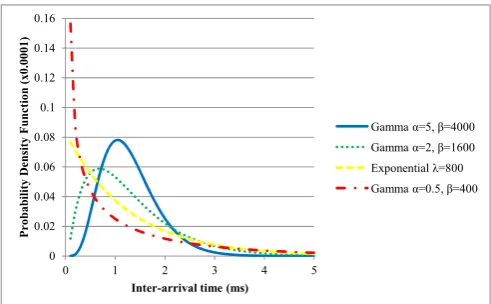
where 0 is the shape parameter, 0 is the rate parameter and Γ ∙ is the gamma function. The gamma distribution was chosen primarily because the exponential distribution is a special case (when 1) and it facilitates understanding of the effect of overdispersion (i.e., larger variance than the exponential distribution with the same mean) when 0 1 and underdispersion (i.e., lower variance than the exponential distribution with the same mean) when 1. Although real M2M applications are characterised by a variety of inter-arrival distribution models, validating the theoretical models for a single exponential (and therefore non-memoryless) distribution such as the gamma distribution provides confidence in their generic nature.

The probability density functions for three different parameterizations of the gamma inter-arrival distribution all having the same mean value ⁄ 1/800 seconds are compared in Fig. 6, along with that of the exponential inter-arrival distribution with an identical mean value 1⁄ 1/800

seconds. Alternatively, we can say the long term arrival rate of all four distributions is 800 packets/second. We employ these specific distributions in a part of the validation along with a maximum service capacity of 10 packets and a persistent allocation period 10 which equates to a load of ⁄ 0.8. Another part of the validation involves examining the effect of changing the load ; for the exponential distribution, we facilitate this by changing the rate parameter appropriately, whereas for the gamma distribution, we maintain the set values of the shape parameter and vary the rate parameter to realise a required rate / .

Fig. 6: Comparison of the Pdf of the Gamma and Exponential

Distributions with the Same Mean

The count model for the gamma distribution assuming the stochastic process begins at the same time as the counting process is given in [28]. With reference to Eq. (11), the count model can be specified as:

Δ , Δ , Δ ₍₂₀₎

, Δ 1

Γ

, Δ Γ

where γ ∙ is the lower incomplete gamma function.

We employ the following predictive adaptation function

, to validate the adaptive persistent uplink resource allocation model:

, min , (21)

is the expected number of packet arrivals during , therefore is the expected queue size at the next persistent allocation epoch given that the queue size immediately after the previous persistent allocation epoch was . The predictive adaptation function , represented by Eq. (21) therefore attempts to reserve just enough resources at the next persistent allocation epoch to serve the conditional expected queue size at that epoch, subject to the constraint that a maximum of packets can be served at any one epoch.

The use of Eq. (21) assumes both the device and base station know the true value of the packet inter-arrival rate . In a real deployment, such a priori knowledge is unlikely, therefore an estimate of is more likely to be employed. This estimate may or may not be updated dynamically based upon real time measurements of packet transfer rate, but clearly both the device and base station must use the same estimated value at any arbitrary point in time.

[image:9.595.43.289.463.615.2]

B.Queue size L

Fig. 7 illustrates the probability mass function (pmf) of queue size for different values of Δ , the time since the previous persistent allocation epoch. Five values of Δ are employed for static persistent allocation, but for display clarity, only the minimum and maximum of these values are used for adaptive persistent allocation. These plots are for =10,

10 , Poisson arrivals (i.e., exponentially distributed packet inter-arrivals) and ⁄ 0.8.

The developed statistical models for the pmf of the queue size exhibit excellent agreement with the results of the simulation. As Δ increases, the expected value of the queue size increases and its distribution becomes more normal in shape. As expected, the queue size for adaptive allocation is on average larger than for static allocation. This is because, with adaptive allocation, there are instances when the calculated instantaneous service capacity is less than the maximum , but, due to a relatively large number of packet arrivals after the service capacity is calculated, the complete device queue cannot be served at the next persistent allocation epoch. In the same scenario with static allocation, it may be possible to serve the complete device queue with a fixed service capacity of . 0

0.02 0.04 0.06 0.08 0.1 0.12 0.14 0.16

0 1 2 3 4 5

Probab

ility

D

ens

ity Function (x

0.0001)

Inter-arrival time (ms)

Gamma α=5, β=4000

Gamma α=2, β=1600

Exponential λ=800

(10)

[image:10.595.43.289.87.235.2]

Fig. 7: Pmf of Queue Size for Different Values of Δt

[image:10.595.308.553.245.392.2]

10, 10 , Poisson arrivals and 0.8

Fig. 8 illustrates the pmf of queue size for different values of and Δ 10 , 10 and Poisson arrivals. We focus on Δ because it corresponds to the instant before the persistent allocation epoch and therefore the queue size is at its maximum; this is the most interesting case from a queue dimensioning perspective. Four values of are employed for static persistent allocation, but for display clarity, only two of these values are used for adaptive persistent allocation. Again the developed statistical models for the pmf of the queue size exhibit excellent agreement with the results of the simulation. As approaches unity, the pmf of becomes increasingly skewed to the right which is to be expected as the system is approaching instability and unbounded growth in the queue size. For 0.95, the graphs for static and adaptive allocation schemes are identical (even though this is not explicitly shown) because the predictive adaptation function employed for this validation always returns a value of under these circumstances.

Fig. 8: Pmf of Queue Size for Different Values of

10, 10 , Poisson arrivals and Δ

Fig. 9 illustrates the probability mass function (pmf) of queue size for different packet inter-arrival distributions and

Δ 10 , 10 and 0.8. Four packet inter-arrival distributions are employed for static persistent allocation, but for display clarity, only two of these, the most

extreme under dispersed and over dispersed parameterizations of the gamma distribution, are used for adaptive persistent allocation. The developed statistical models for the pmf of the queue size exhibit excellent agreement with the results of the simulation for all studied parameterizations of the gamma distribution. Unsurprisingly, for over dispersed parameterizations of the gamma distribution (i.e., 0 1), the distribution of the queue size is also over dispersed with respect to the case of exponentially distributed packet inter-arrival times. Similarly, for under dispersed parameterizations of the gamma distribution (i.e., 1), the distribution of the queue size is also under dispersed with respect to the case of exponentially distributed packet inter-arrival times.

Fig. 9: Pmf of Queue Size for Different Packet Inter-Arrival Distributions 10, 10 , 0.8 and Δ )

C.Delay

Fig. 10 illustrates the marginal pdf of delay for different values of . These plots are for 10, 10 ,

/10 1 and Poisson arrivals. Four values of are employed for static persistent allocation, but for display clarity, only two of these values are used for adaptive persistent allocation. The developed statistical models for the pdf of the marginal delay clearly exhibit excellent agreement with the results of the simulation.

For the static allocation scheme, we see that for a relatively small load (e.g. 0.5), the delay pdf appears to be almost

uniform i.e., ~ , . This is

expected because with a small load, almost all packet arrivals can be served at the very next persistent allocation epoch, and the delay is then only determined by the waiting time

to that next epoch which is itself uniformly distributed for Poisson arrivals. As the load increases, the queue size increases and there is a greater probability that packets cannot be served at the very next persistent allocation epoch after they arrive. Consequently the pdf decreases for and increases for . In general, the pdf exhibits a significant sharp reduction as the delay surpasses , such that the shape of the pdf as a whole resembles a “shark fin”. This suggest that it might be possible to model the pdf as two piecewise functions, one either side of the discontinuity, although we do not consider this further in 0

0.1 0.2 0.3 0.4 0.5 0.6 0.7 0.8

0 5 10 15 20

pr

obab

ilit

y

Queue size L in packets

Static simulation Δt=0 Static theory Δt=0 Static simulation Δt=0.25*τperiod Static theory Δt=0.25*τperiod Static simulation Δt=0.5*τperiod Static theory Δt=0.5*τperiod Static simulation Δt=0.75*τperiod Static theory Δt=0.75*τperiod Static simulation Δt=τperiod Static theory Δt=τperiod Adaptive simulation Δt=0 Adaptive theory Δt=0 Adaptive simulation Δt=τperiod Adaptive theory Δt=τperiod

0 0.02 0.04 0.06 0.08 0.1 0.12 0.14 0.16 0.18

0 5 10 15 20 25 30

p

rob

ab

il

it

y

Static simulation ρ=0.5 Static theory ρ=0.5 Static simulation ρ=0.8 Static theory ρ=0.8 Static simulation ρ=0.9 Static theory ρ=0.9 Static simulation ρ=0.95 Static theory ρ=0.95 Adaptive simulation ρ=0.5 Adaptive theory ρ=0.5 Adaptive simulation ρ=0.9 Adaptive theory ρ=0.9

0 0.05 0.1 0.15 0.2 0.25 0.3

0 5 10 15 20 25 30

pr

ob

abil

it

y

Static simulation (Gamma α=5, β=4000)

Static theory (Gamma α=5, β=4000)

Static simulation (Gamma α=2 β=1600)

Static theory (Gamma α=2, β=1600)

Static simulation (Exponential λ=800)

Static theory (Exponential λ=800)

Static simulation (Gamma α=0.5, β=400)

Static theory (Gamma α=0.5, β=400)

Adaptive simulation (Gamma α=5, β=4000)

Adaptive theory (Gamma α=5, β=4000)

Adaptive simulation (Gamma α=0.5, β=400)

[image:10.595.43.291.486.634.2]

(11)

this paper. It also demonstrates the complexity of the delay pdf even when the simple Poisson arrival process is considered.

For the adaptive allocation scheme, the shape of the delay pdf resembles a shark fin for both small and high loads. This is a consequence of attempting to use the minimum amount of allocated resources to serve the expected queue size at the next persistent allocation epoch. This also explains why the expected delay is larger for the adaptive allocation scheme than the static allocation scheme.

[image:11.595.306.553.122.268.2]

Note also that for 0.95, as with the queue size , the graphs for static and adaptive allocation schemes are identical (even though this is not explicitly shown) because the predictive adaptation function employed for this validation always returns a value of under these circumstances.

Fig. 10: Marginal Pdf of Delay for Different Values of

10, 10 , /10 and Poisson arrivals

[image:11.595.42.290.258.403.2]

For completeness, Fig. 11 illustrates the marginal cumulative distribution function (cdf) of delay for different values of that corresponds to the pdf plots in Fig. 10.

Fig. 11: Marginal Cdf of Delay for Different Values of

10, 10 , /10 and Poisson arrivals

Fig. 12 illustrates the marginal pdf of delay for different packet inter-arrival distributions and 10 ,

10 and 0.8. Four packet inter-arrival distributions are employed for static persistent allocation, but for display clarity, only two of these, the most extreme under dispersed and over

dispersed parameterizations of the gamma distribution, are used for adaptive persistent allocation.

Fig. 12: Marginal Pdf of Delay for Different Packet Inter-Arrival

Distributions 10, 10 , /10 and

0.8)

The developed statistical models for the pdf of the marginal delay clearly exhibit excellent agreement with the results of the simulation for all studied parameterizations of the gamma distribution. Similarly to the discussion on queue size , for over dispersed parameterizations of the gamma distribution (i.e., 0 1), the marginal pdf of delay is also over dispersed with respect to the case of exponentially distributed packet inter-arrival times. Similarly, for under dispersed parameterizations of the gamma distribution (i.e., 1), the marginal pdf of delay is also under dispersed with respect to the case of exponentially distributed packet inter-arrival times and in fact tends towards a uniform distribution. This is because there is less chance of relatively short inter-arrivals time with an under dispersed distribution and therefore almost all packet arrivals can be served at the very next persistent allocation epoch, so the delay is then only determined by the waiting time to that next epoch.

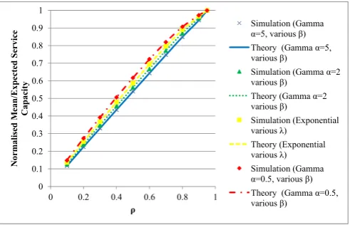
D.Expected Service Capacity E{G} for Adaptive Allocations Recall from Section II.B that the instantaneous service capacity is a random variable that represents the volume of resources on the uplink data channel dedicated to an adaptive persistent resource at an arbitrary persistent allocation epoch. Fig. 13 illustrates the normalized expected service capacity

/ as a function of for different packet inter-arrival distributions when using adaptive persistent uplink resource allocation. This plot is for 10, 10 and

/10 1 . There is close agreement between the theoretical statistical model and the simulation results.

As expected, for small values of , the instantaneous service capacity calculated by the adaptation function is in general less than since fewer resources are required to serve the offered traffic, therefore / is correspondingly smaller. As increases, / also increases in sympathy although the relationship is not strictly linear. This plot demonstrates an advantage of the adaptive scheme over the static scheme in that resources can be allocated more efficiently

0 0.01 0.02 0.03 0.04 0.05 0.06 0.07 0.08 0.09 0.1 0.11

0 5 10 15 20 25 30

pdf

Delay in number of slots

Static simulation ρ=0.5

Static theory ρ=0.5

Adaptive simulation ρ=0.5

Adaptive theory ρ=0.5

0 0.1 0.2 0.3 0.4 0.5 0.6 0.7 0.8 0.9 1

0 5 10 15 20 25 30

cdf

0 0.01 0.02 0.03 0.04 0.05 0.06 0.07 0.08 0.09 0.1 0.11

0 5 10 15 20 25 30

pd

f

Static simulation (Gamma

α=5, β=4000) Static theory (Gamma α=5,

β=4000)

α=2 β=1600)

Static theory (Gamma α=2,

β=1600) Static simulation (Exponential λ=800) Static theory (Exponential

λ=800)

α=0.5, β=400) Static theory (Gamma

α=0.5, β=400) Adaptive simulation (Gamma α=5, β=4000) Adaptive theory (Gamma

α=5, β=4000) Adaptive simulation (Gamma α=0.5, β=400) Adaptive theory (Gamma

[image:11.595.43.290.485.640.2]

(12)

[image:12.595.44.290.167.325.2]

as the expected service capacity for an adaptive allocation is always less than required by a static allocation for 1. Furthermore, the adaptive scheme can automatically adapt to changes in the packet inter-arrival distribution or the load without expensive signalling on the downlink control channels.

Fig. 13: Normalized Expected Service Capacity / for Different Values of and Adaptive Allocation

=10, 10 and /10

For over dispersed parameterizations of the gamma distribution (i.e., 0 1), the normalized expected service capacity / for an arbitrary value of is larger than for exponentially distributed packet inter-arrival times. This is to be expected because there is a greater chance of larger queue sizes in such cases (see Section IV. B). For under dispersed parameterizations of the gamma distribution (i.e., 1), the the normalized expected service capacity / for an arbitrary value of is smaller than the case of exponentially distributed packet inter-arrival times. Again this is to be expected because there is a lower chance of larger queue sizes in such cases.

For completeness, we note that, in terms of the downlink assignment control channel, there is no difference in resource savings between static and adaptive persistent resource allocations since only a single assignment message is required for both when they are first established.

E.Additional Results

When dimensioning a persistent resource allocation for a given source with a given packet inter-arrival distribution, there are two parameters of the allocation which can be assigned independently: the transmission opportunity period and the (maximum) amount of allocated resources per transmission opportunity. Therefore it is possible to maintain a certain desired load ⁄ with different pairs of and values which have a constant ratio. The choice of values to employ depends upon such factors as the delay budget, jitter tolerance and desired duty cycle of the source. In this section, we demonstrate that the theoretical models predict the correct queue size and delay distributions for different pairs of and values for a target desired load .

[image:12.595.304.555.193.342.2]

Fig. 14 illustrates the probability mass function (pmf) of queue size for different pairs of and values such that ⁄ 0.8 for a constant packet inter-arrival rate of 800 packets/second. Fig. 15 illustrates the marginal pdf of delay under the same conditions. Four pairs of and values are employed for static persistent allocation, but for display clarity, only two of these, the smallest and largest pairs, are used for adaptive persistent allocation.

[image:12.595.305.551.372.522.2]

Fig. 14: Pmf of Queue Size for Different Values of and Poisson arrivals, 0.8 and Δ )

Fig. 15: Marginal Pdf of Delay for Different Values of and Poisson arrivals, 0. 8 and 1 )

Unsurprisingly, as (and ) increase, the expected queue size and delay also increase on account of the fact that generated packets must wait longer on average until the next persistent allocation epoch. For the static allocation scheme, the delay pdf tends to a uniform distribution i.e.,

~ , as increases. This

is expected because almost all packet arrivals can be served at the very next persistent allocation epoch, and the delay is then only determined by the waiting time to that next epoch which is itself uniformly distributed for Poisson arrivals. For the adaptive allocation scheme, the shape of the delay pdf becomes more uniform in shape as increases but still resembles a shark fin. This is a consequence of attempting to use the minimum amount of allocated resources to serve the expected queue size at the next persistent allocation epoch.

0 0.1 0.2 0.3 0.4 0.5 0.6 0.7 0.8 0.9 1

0 0.2 0.4 0.6 0.8 1

No rmal is ed M ean /E xp ec te d S er vi ce Ca pac it y ρ Simulation (Gamma

α=5, various β)

Theory (Gamma α=5,

various β)

Simulation (Gamma α=2

various β)

Theory (Gamma α=2

various β)

Simulation (Exponential

various λ)

Theory (Exponential

various λ)

Simulation (Gamma

α=0.5, various β)

Theory (Gamma α=0.5,

various β)

0 0.02 0.04 0.06 0.08 0.1 0.12 0.14 0.16 0.18

0 10 20 30 40

pr

ob

abi

li

ty

Static simulation ψ=5

τperiod=5ms Static theory ψ=5

τperiod=5ms Static simulation ψ=10

τperiod=30ms Adaptive simulation ψ=5

τperiod=5ms Adaptive theory ψ=5

τperiod=30ms 0 0.02 0.04 0.06 0.08 0.1 0.12 0.14 0.16 0.18 0.2

0 10 20 30 40

pdf

Static simulation ψ=5

(13)

This also again explains why the expected delay is larger for the adaptive allocation scheme than the static allocation scheme.

V.CONCLUSIONS

In this paper, we have derived theoretical statistical models to represent the queue size and packet delay for static and adaptive persistent uplink resource allocations provided to M2M applications with an arbitrary non-deterministic packet arrival process sending small packets over wireless systems. These theoretical models were shown to exhibit very close agreement with the queue size and packet delay statistics obtained from a custom discrete event simulation model, both when using exponential and gamma distributed packet inter-arrivals. The packet delay distribution is quite complex in general even when a simple packet arrival process such as the Poisson arrival process is considered. An adaptive persistent uplink resource allocation scheme utilises resources more efficiently than a static persistent uplink resource allocation scheme at the expense of increased expected queue size and increased expected packet delay. The performance difference depends upon the exact adaptation function in use at the device and base station to calculate the instantaneous service capacity at the next transmission opportunity based upon the remaining queue size at the previous transmission opportunity. An additional advantage of the adaptive allocation scheme is that it automatically adapts to changes in the nature of the packet arrival process (e.g. start/stop transmission) without requiring expensive signalling on control channels.

The primary motivation of this work has been to facilitate dimensioning of persistent resource allocations given a set of QoS requirements, in particular those related to delay. By employing the statistical models developed in this paper, the base station can determine the period and (maximum) volume of persistent resources required to meet a given delay budget a certain percentage of the time.

One item of future work will be to characterize the tradeoff between delay and resource allocation efficiency in using different adaptation functions for adaptive persistent uplink resource allocations. The predictive adaptation function employed for model validation in this paper attempts to match the instantaneous volume of resources with the conditional expected queue size at each transmission opportunity, however this does result in some resource wastage when fewer packets are generated between transmission opportunities than expected. A less aggressive predictive adaptation function or non-predictive adaptation function will result in less resource wastage at the expense of higher expected delay.

ACKNOWLEDGMENT

This work has been supported by Ausgrid and the Australian Research Council (ARC). Jason Brown would like to thank Joanne Simpson for providing inspiration during the writing of this paper.

REFERENCES

[1] Patel, A.; Aparicio, J.; Tas, N.; Loiacono, M.; Rosca, J., "Assessing communications technology options for smart grid

applications," Smart Grid Communications (SmartGridComm), 2011 IEEE International Conference on, pp.126,131, 17-20 Oct. 2011, doi: 10.1109/SmartGridComm.2011.6102303

[2] Shafiq, M.Z.; Lusheng Ji; Liu, A.X.; Pang, J.; Jia Wang, "Large-Scale Measurement and Characterization of Cellular Machine-to-Machine Traffic," Networking, IEEE/ACM Transactions on, vol. 21, no. 6, pp. 1960-1973, Dec. 2013, doi: 10.1109/TNET.2013.225643

[3] Kuzlu, M.; Pipattanasomporn, M., "Assessment of

communication technologies and network requirements for different smart grid applications," Innovative Smart Grid Technologies (ISGT), 2013 IEEE PES, pp.1,6, 24-27 Feb. 2013, doi: 10.1109/ISGT.2013.6497873

[4] Potsch, T.; Khan Marwat, S.N.; Zaki, Y.; Gorg, C., "Influence of future M2M communication on the LTE system," Wireless and Mobile Networking Conference (WMNC), 2013 6th Joint IFIP pp.1-4, 23-25 April 2013, doi: 10.1109/WMNC.2013.6549000 [5] Ghavimi, F.; Chen, Hsiao-Hwa, "M2M Communications in

3GPP LTE/LTE-A Networks: Architectures, Service Requirements, Challenges and Applications," Communications Surveys & Tutorials, IEEE , October 2014, doi: 10.1109/COMST.2014.2361626

[6] Khan, R.H.; Mahata, K.; Brown, J., "An adaptive RRM scheme for smart grid M2M applications over a WiMAX network," Communication Systems, Networks & Digital Signal Processing (CSNDSP), 2014 9th International Symposium on, pp.820-825, 23-25 July 2014, doi: 10.1109/CSNDSP.2014.6923940

[7] 3GPP TS 22.368 V12.4.0 (2014-06), “Service requirements for Machine-Type Communications (MTC), Stage 1”, Release 12 [8] IEEE 802.16p-2012, “IEEE Standard for Air Interface for

Broadband Wireless Access Systems-Amendment 1: Enhancements to Support Machine-to-Machine Applications” [9] Laya, A.; Alonso, L.; Alonso-Zarate, J., "Is the Random Access

Channel of LTE and LTE-A Suitable for M2M Communications? A Survey of Alternatives," Communications Surveys & Tutorials, IEEE, vol.16, no.1, pp.4-16, 1Q 2014, doi: 10.1109/SURV.2013.111313.00244

[10]Hasan, M.; Hossain, E.; Niyato, D., "Random access for machine-to-machine communication in LTE-advanced networks: issues and approaches," Communications Magazine, IEEE, vol.51, no.6, pp.86-93, June 2013, doi: 10.1109/MCOM.2013.6525600

[11]Jason Brown, Jamil Y. Khan, “Key performance aspects of an LTE FDD based Smart Grid communications network”, Computer Communications, Volume 36, Issue 5, 1 March 2013, Pages 551-561, ISSN 0140-3664, doi: 10.1016/j.comcom.2012.12.007.

[12]Shao-Yu Lien; Kwang-Cheng Chen, "Massive Access

Management for QoS Guarantees in 3GPP Machine-to-Machine Communications," Communications Letters, IEEE, vol. 15, no. 3, pp. 311-313, March 2011, doi: 10.1109/LCOMM.2011.011811.101798

[13]You, Chunhua; Zhang, Yuan, "A radio resource scheduling scheme for periodic M2M communications in cellular networks," Wireless Communications and Signal Processing (WCSP), 2014 Sixth International Conference on, pp.1-5, 23-25 Oct. 2014, doi: 10.1109/WCSP.2014.6992085

[14]Gotsis, Antonis G.; Athanasios S. Lioumpas; Angeliki Alexiou.; "Analytical modelling and performance evaluation of realistic time‐controlled M2M scheduling over LTE cellular networks." Transactions on Emerging Telecommunications Technologies 24, no. 4 (2013): pp. 378-388, doi: 10.1002/ett.2629

(14)

802.16e system," Personal Indoor and Mobile Radio Communications (PIMRC), 2010 IEEE 21st International Symposium on, pp.1481,1486, 26-30 Sept. 2010, doi: 10.1109/PIMRC.2010.5671974

[16]3GPP TS 36.321 V8.10.0 (2011-09), “Evolved Universal

Terrestrial Radio Access (E-UTRA); Medium Access Control (MAC) protocol specification”, Release 10

[17]oneM2M, oneM2M-TR-0001-UseCase, “oneM2M Use cases

collection”, v0.0.5, 23 September 2013

[18]Afrin, Nusrat; Brown, Jason; Khan, Jamil Y., "An Adaptive Buffer Based Semi-persistent Scheduling Scheme for Machine-to-Machine Communications over LTE," Next Generation Mobile Apps, Services and Technologies (NGMAST), 2014 Eighth International Conference on, pp.260-265, 10-12 Sept. 2014, doi: 10.1109/NGMAST.2014.48

[19]Lam, S., "Delay Analysis of a Time Division Multiple Access (TDMA) Channel," Communications, IEEE Transactions on, vol.25, no.12, pp.1489-1494, Dec 1977, doi: 10.1109/TCOM.1977.1093784

[20]Rubin, I., "Message Delays in FDMA and TDMA

Communication Channels," Communications, IEEE Transactions on, vol.27, no.5, pp.769-777, May 1979, doi: 10.1109/TCOM.1979.1094462

[21]King-Tim Ko; Davis, B.R., "Delay Analysis for a TDMA Channel with Contiguous Output and Poisson Message Arrival," Communications, IEEE Transactions on, vol.32, no.6, pp.707-709, Jun 1984, doi: 10.1109/TCOM.1984.1096126

[22]Bruneel, H., "Message Delay in TDMA Channels with

Contiguous Output," Communications, IEEE Transactions on , vol.34, no.7, pp.681,684, Jul 1986, doi: 10.1109/TCOM.1986.1096608

[23]Rubin, I.; Zhang, Z., "Message delay analysis for TDMA schemes using contiguous-slot assignments," Communications, IEEE Transactions on, vol.40, no.4, pp.730-737, Apr 1992, doi: 10.1109/26.141428

[24]Khan, K.; Peyravi, H., "Delay and queue size analysis of TDMA with general traffic," Modeling, Analysis and Simulation of Computer and Telecommunication Systems, 1998. Proceedings. Sixth International Symposium on, pp.217-225, 19-24 Jul 1998, doi: 10.1109/MASCOT.1998.693698

[25]Sheldon M. Ross, “Introduction to Probability Models”, 10th edition, Academic Press, 2009

[26]Drajic, D.; Krco, S.; Tomic, I.; Svoboda, P.; Popovic, M.; Nikaein, N.; Zeljkovic, N., "Traffic generation application for simulating online games and M2M applications via wireless networks," Wireless On-demand Network Systems and Services (WONS), 9th_{Annual Conference on, pp.167-174, 9-11 Jan.}

2012, doi: 10.1109/WONS.2012.6152224

[27]Ilker Demirkol, Cem Ersoy, Fatih Alagöz, Hakan Deliç, “The impact of a realistic packet traffic model on the performance of surveillance wireless sensor networks”, Computer Networks, Volume 53, Issue 3, 27 February 2009, Pages 382-399, ISSN 1389-1286, doi: 10.1016/j.comnet.2008.10.021.

[28]Ploennigs, J.; Neugebauer, M.; Kabitzsch, K., "A traffic model for networked devices in the building automation," Factory Communication Systems, 2004. Proceedings. 2004 IEEE International Workshop on, pp.137-145, 2004, doi: 10.1109/WFCS.2004.1377694

[29]Winkelmann, Rainer. "Duration dependence and dispersion in count-data models." Journal of Business & Economic Statistics 13, no. 4 (1995): 467-474.

[30]McShane, Blake, Moshe Adrian, Eric T. Bradlow, and Peter S. Fader. "Count models based on weibull interarrival times." Journal of Business & Economic Statistics 26, no. 3 (2008).

[31]DR Cox, “Renewal Theory”, Methuen’s Monographs on

Applied Probability and Statistics, 1962

Jason Brown received his BEng and Ph.D. from the University of Manchester Institute of Science and Technology (UMIST) in 1990 and 1994 respectively. He has worked in R&D and operational roles for Vodafone, AT&T and LG Electronics. In 2011, he joined the University of Newcastle in Australia researching smart grid and M2M communications technologies. His main research interest areas are 4G and 5G wireless networks, smart grid communications, M2M communications and wireless sensor networks.

Nusrat Afrin is a PhD student in the University of Newcastle, Australia. She completed her Bachelors of Science in Electrical and Electronic Engineering in 2009 from Bangladesh University of Engineering and Technology. After that she worked for two and a half years in the telecommunication industries of Bangladesh. Since 2012, she has been pursuing her PhD studies in Electrical Engineering in the University of Newcastle, Australia. Her research interests include LTE, machine-to-machine communications, packet scheduling and MAC and cross layer designs.