Estimating models for panel survey data under complex sampling

E

STIMATING

M

ODELS FOR

P

ANEL

S

URVEY

D

ATA UNDER

C

OMPLEX

S

AMPLING

M

ARCEL

D.

T.

V

IEIRA

,

C

HRIS

J.

S

KINNER

A

BSTRACT

Complex designs are often used to select the sample which is followed over time in a

panel survey. We consider some parametric models for panel data and discuss methods

of estimating the model parameters which allow for complex schemes. We incorporate

survey weights into alternative point estimation procedures. We also consider variance

estimation using linearization methods to allow for complex sampling, and indicate

connections with established asymptotically distribution free (ADF) methods. The

behaviour of the proposed inference procedures are assessed in a simulation study, based

upon data from the British Household Panel Survey. There appear to be some

advantages of using the weighted maximum likelihood (ML) point estimation method

compared to the weighted ADF method. Variance estimation methods that allow for

clustering tend to lead to improvements in terms of bias. However, the variance

estimator for the weighted ML estimator performs better than the ADF variance

estimators.

Southampton Statistical Sciences Research Institute

Estimating Models for Panel Survey Data under Complex

Sampling

Marcel D. T. Vieira

Universidade Federal de Juiz de Fora

Departamento de Estatística, Juiz de Fora, 36036-330, MG, Brazil

and

Chris J. Skinner

University of Southampton

Division of Social Statistics, Southampton, SO17 1BJ, United Kingdom

Abstract. Complex designs are often used to select the sample which is followed over time in a panel survey. We consider some parametric models for panel data and discuss methods of estimating the model parameters which allow for complex schemes. We incorporate survey weights into alternative point estimation procedures. We also consider variance estimation using linearization methods to allow for complex sampling, and indicate connections with established asymptotically distribution free (ADF) methods. The behaviour of the proposed inference procedures are assessed in a simulation study, based upon data from the British Household Panel Survey. There appear to be some advantages of using the weighted maximum likelihood (ML) point estimation method compared to the weighted ADF method. Variance estimation methods that allow for clustering tend to lead to improvements in terms of bias. However, the variance estimator for the weighted ML estimator performs better than the ADF variance estimators.

Acknowledgment: This work was partially supported by the Brazilian National Council for Scientific and Technological Development (CNPq) grant 200286/01.3.

1. Introduction

A broad class of ‘regression-type’ models has found a wide range of useful applications with panel survey data (Baltagi, 2001; Wooldridge, 2001; Diggle et al., 2002; Hsiao, 2003). Such data often consist of repeated observations on the same variables for the same individuals across equally spaced waves of data collection. The ‘regression-type’ models considered here are broadly concerned with representing the relationship between one of the variables, treated as dependent, and a number of the other variables, treated as covariates. A typical example of the kind of panel survey considered here is the British Household Panel Survey (BHPS), in which a sample of households was selected at wave one and then individuals in this sample were followed up repeatedly at annual intervals.

It is common for the selection of the initial panel sample at wave one to involve a complex sampling scheme. For example, stratification and multistage sampling were employed in the selection of the initial BHPS sample. In addition, sample individuals are often selected with unequal probabilities and weights are constructed to compensate for these unequal probabilities as well as for different forms of wave nonresponse and other complexities (Kalton and Brick, 2000). There is a limited consideration of the treatment of such sampling schemes in the panel data model literature, especially in relation to the clustering of individuals (Wooldridge, 2001).

have therefore been developed in the cross section data model context, and include for example a pseudo maximum likelihood approach for point estimation, and linearization methods for variance estimation.

In this paper we shall extend these methods to consider estimation of panel data models parameters, allowing for complex sampling designs. We shall discuss methods of statistical inference for models with parametric assumptions about the covariance structure of errors over time. We shall incorporate survey weights into alternative point estimation procedures, including maximum likelihood, generalized least squares and asymptotically distribution free (ADF) approaches. We shall also consider standard error estimation approaches using Taylor series linearization methods to allow for complex sampling, and indicate connections with some established ADF methods. We shall adopt an aggregate modelling strategy (Skinner, Holt and Smith, 1989) rather than a multilevel covariance modelling approach. For developments of the latter approach see Müthén and Satorra (1995, Section 5).

Some previous work on estimation for panel data models under complex designs has been undertaken by Feder, Nathan and Pfeffermann (2000), who propose combining multilevel modelling, time series modelling and survey sampling methods; Sutradhar and Kovacevic (2000), where a generalised estimating equations approach is developed by considering an autocorrelation structure in a multivariate polytomous longitudinal survey data context; Skinner and Holmes (2003), who study two approaches for dealing with sampling effects, either considering the repeated observations as multivariate outcomes and adopting weighted estimators that account for the correlation structure, or considering a two-level longitudinal model and to modify weighting strategy proposed by Pfeffermann et al. (1998); and Skinner and Vieira (2005), who presented some empirical evidence that the variance-inflating impacts of complex sampling schemes can be higher for longitudinal analyses than for corresponding cross-sectional analyses.

estimation of covariance matrices are reviewed in Section 4. Estimation of model parameters using least squares methods and pseudo maximum likelihood estimation are also considered. The paper proceeds in Section 5 to consider variance estimation methods, by adopting Taylor series linearization methods to allow for complex sampling and also considering ADF variance estimation techniques. Two simulation studies, based upon data from the British Household Panel Survey, will be presented in Section 6 to assess the behaviour of the different estimation procedures. We make brief remarks in the concluding discussion in Section 7.

2. Sampling and Data

We suppose that the data consist of the values y_itof an outcome variable and 1×q vectors of values

it

x of covariates for each individual i in a sample, denoted s, and each wave of data collection

1, ,

t= T. The sample is assumed to be selected from a specified finite population at wave 1

according to a probability design for which the inclusion probability π_i of each individual i in s is

known and the sample and the population are fixed thereafter. We suppose that sampling

weights,w_i, are available for estimation and that, by default, these are the reciprocals of the sample

inclusion probablities πi. We shall sometimes write s={1,..., }n , without loss of generality, where n

is the sample size. For simplicity, we shall not refer to nonresponse, treating the data as complete. In practice, this will not be the case and s may be interpreted as the set of individuals providing

values y_it and x_it at each occasion, where the w_i include some adjustment for nonresponse.

3. Models

We consider standard kinds of models for the repeated measurements (Ware, 1985; Diggle et al.,

2002, Chapters 4 and 5; among others) in which the y_it obey the linear model:

( )

yit xit

where x_it is treated as fixed (or conditioned upon), is a q×1 vector of unknown parameters (and

we make no distinction between the realised y_it and the underlying random variables). We allow

for serial correlation in the measurements by writing the repeated measurements for individual i as

the T×1 vector y_i =

(

y_i1,,y_iT

)

′ and allowing for non-zero off-diagonal elements of the

covariance matrix Σ of this vector:

Σ=cov

( )

yi = E{[yi −Xi ][yi −Xi ]′}, (2)

where Xi=

(

xi1´,,xiT´

)

´ is the T×q matrix of covariate values.

We consider two possible structures for the matrix Σ. The first is referred to as the uniform

correlation model (UCM), where all the off-diagonal elements of Σ are 2 u

σ and all the diagonal

elements are 2 2 u v

σ +σ . This corresponds to the multilevel model:

it i it

it u v

y =x + + (3)

where u_i and v_it are random effects with zero means and variances 2 u

σ and 2 v

σ respectively, which

are uncorrelated over time. In this case the correlation between y_it and y_it’ for any two occasions t

and ’t for t t≠ ’ is given by 2_/( 2 2₎ u u v

ρ σ σ= +σ .

In our second structure, referred to as the AR1 model, the correlation is allowed to decay over

time. We again assume that all diagonal elements are 2 2 u v

σ +σ but now suppose that the covariance

between y_it and y_it’ for occasions t and ’t takes the form _{cov(y , )} 2 t t 2 it yit σu γ σv

′ −

′ = + , where γ is an

additional parameter (| | 1γ < ). This model corresponds to the following first-order autoregressive

process for the v_it:

it it it v

v =γ −1+ε , (4)

where the εit are mutually independent residuals with zero mean and variance σε2 = −(1 γ σ)2 v2

To emphasise the fact that the covariance matrix Σ takes a particular parametric structure for

each model, we write Σ=Σ

( )

, where is a b×1 parameter vector. In particular, =

(

σ2,σ2,γ

)

′

v u

for the AR1 model and =

(

2_, 2

)

′ v u σ

σ for the UCM model. Note that the UCM model is a special

case of the AR1 model where γ =0.

We have so far only made assumptions about the correlation of the yit between different time

points t but not between different individuals i. We shall, indeed, assume that the parameter vector

governing the inter-temporal covariance matrix Σ

( )

is of scientific interest, but that any

correlation between values of y_it for different individuals is a ‘nuisance’ . In the UCM and AR1

models we shall assume that the correlation between y_it and y_{i t’ ’} is zero for any two distinct

individuals i and ’i and any two occasions t and ’t . We shall also consider a UCM(C) model,

where C denotes cluster, for which this correlation is given by a fixed quantity, τ , for any distinct individuals i and ’i in the same cluster and any two occasions t and ’t and zero otherwise, where

the inter-temporal covariance structure Σ

( )

is the same as for the UCM model.

4. Point Estimation

We shall suppose that is estimated following an established approach for repeated survey

observations, as implemented for example in the software SUDAAN (Shah et al. 1997), by:

∑

∑

∈

− −

∈

− _{ ′}

  



 _′ =

s

i i i i s

i i i i

V X w X

V X

w 1y

1 1

ˆ ₍₅₎

where V is a specified ‘working’ covariance matrix of y_i (Diggle et al. 2002, p.70) and the w_i are

the survey weights introduced in section 2. Provided the linear model in (1) holds and V is

constant, ˆ will be consistent for with respect to the joint model and sampling design if the

In the simulation study we shall suppose that V is estimated using the UCM model as the

working model. This just requires estimating the intra-individual correlation ρ since 2 2 2

u v

σ

=

σ σ

+

cancels out of the two places V appears in (5). We shall estimate the correlation _ρ by iterating

between GLS estimation of and survey-weighted moment-based estimation of the

intra-individual correlation (Liang and Zeger, 1986; Shah et al., 1997). Following standard large sample

arguments (Liang and Zeger, 1986) ˆ will remain consistent for even though V is subject to

sampling variation.

As in section 3, let denote the b×1 vector of parameters of interest which determine the covariance structure Σ=Σ

( )

of yi, as given in (2). In order to define a class of estimators , we

first define the weighted residual covariance matrix:

(

)(

)

∑

∈

− _{− −} ′

=

s

i i i i i i

w N w X X

S ˆ 1 y ˆ y ˆ ₍₆₎

where

∑

=

= n

i i

w N

1

ˆ _{estimates the population size, N. The matrix Sw is a consistent estimator of Σ with}

respect to the joint model and sampling design, provided that the model assumptions in (1) and (2)

hold (Skinner, Holt and Smith, 1989). Having defined S_w, we now define the class of estimators ˆ

of to be considered, as those that minimise different measures of ‘distance’ between S_w and Σ

( )

ˆ

(Jöreskog and Goldberger, 1972; Browne, 1984; Bollen, 1989). More precisely, if F

(

Sw,Σ

)

denotes

the fitting function, which measures the distance between S_w and Σ, then ˆ is defined as the value

of which minimises F

(

S_w,Σ

( )

)

across values of in a specified b-dimensional parameter

space.

The simplest example of a fitting function is the unweighted least squares (ULS) function:

( )

{[ ] }

2 1

,_{Σ = ⋅tr S−Σ} 2

S

The resulting ULS estimator ˆ is uniquely defined and is consistent for , given that _ULS S_w is

consistent for Σ (Browne, 1982; Browne, 1984). However, ˆ is not in general an asymptotically ULS

efficient estimator of . Moreover, it is not scale invariant (Jöreskog and Goldberger, 1972)

although this does not seem a serious problem when the elements of y_i are repeated measurements

of the same variable. With the aim of improving efficiency, we consider also a class of generalised least squares fitting functions:

{

}

1

{

}

( , ) ( ) ( ) U ( ) ( )

GLS

F S _{Σ =} vech S ₋vech _Σ ′ − vech S ₋vech _{Σ , (8)}

where vech is the vector of distinct elements of a symmetric matrix (Fuller, 1987). For the T T×

matrices considered here, vech is of dimension k×1, where k T T= ( +1) / 2. The ‘weight’ matrix U

remains to be specified. For efficient estimation, we should like U to correspond to (approximately)

to the covariance matrix of vech S( ), for the relevant matrix S, which is S_w in our setting. A

traditional approach to the specification of U, which ignores the complex sampling scheme and is motivated by a working assumption of normality and independent and identically distributed observations, is (McDonald, 1980):

(

W W

)

K K

U =2⋅ ′ ⊗ , (9)

where K is the so-called transition matrix, W is any consistent estimator of Σ (Bentler and Weeks, 1980; Swain, 1975), and ⊗ is the right Kronecker product operator. Expression (9) may alternatively be written elementwise as (Joreskog and Goldberger, 1972; Swain, 1975):

t t tt t t tt t t

tt W W W W

U ′,′′′′′ = ′′ ′ ′′′+ ′′′ ′′′, (10)

where U_{tt′,t′′t′′′} and W_tt′ represent typical elements respectively of U and W.

Expressions (8) and (9) imply (Browne, 1977) that F_GLS( , )S Σ takes the form:

( )

{[

(

)

] }

2 1

, −1 2

− ⋅ −Σ

     =

Σ tr S W S

where GLS-NORM indicates that this choice of fitting function is based upon an underlying

normality assumption. There are two natural choices of W. The first is given by S, since this (S_w in

our setting) is assumed consistent for Σ. In this case we may write:

( )

(

)

{[ ] } 2 1 } ] {[ 2 1

, 1 2 1 2

1 − −

− ⋅ −Σ

     = Σ − ⋅       =

Σ tr S S tr I S S

FGLS NORM . (12)

An alternative choice is to set W equal to Σ, leading to:

( )

{[ ] }

2 1

, 1 2

2 S tr S I

FGLS NORM ⋅ Σ −

     = Σ −

− . (13)

We denote the resulting estimators of as ˆ_GLS−NORM1 and ˆ_GLS−NORM2. An alternative approach,

not based on the working assumption of normality, is to set U equal to an estimator of the

asymptotic covariance matrix of vech S( ), making no assumption about the underlying distribution.

Such an approach is often called asymptotically distribution free (ADF). See e.g. Browne (1982, 1984). We shall consider the use of linearization methods of variance estimation for this purpose in the next section, following some earlier applications of this idea in Skinner (1989), Satorra (1992), and Müthén and Satorra (1995).

Another approach to estimation is achieved by adopting the pseudo-maximum likelihood (PML) approach (Skinner, Holt and Smith, 1989) in which a census log-likelihood (assuming independent and identically distributed observations) is replaced by a weighted log-likelihood given by (ignoring constants):

( )

_∑

( )

∈ − ₋ Σ ′ − − Σ − s

i i i i i i

X X

w

Nlog [ ] 1[ ]

y

y (14)

If this weighted likelihood is first ‘concentrated’ by replacing by ˆ, maximising expression (14)

becomes equivalent to minimising the value of the following fitting function (Jöreskog,1970) :

[ ]

S S T tr

S

with S evaluated at S_w to take account of the complex design. Alternatively, if this initial

concentration does not take place, could be estimated simultaneously with by maximising

expression (14). If N is unknown, it might be replaced in (14) by

∑

=

= n

i i

w N

1

ˆ _.

The properties of the GLS-NORM1 and PML approaches may be compared by noting first that (12) may be alternatively expressed as (see Fuller, 1987, p. 334)

2 1

1 1

( , ) ( 1) ( 1) 2

T

GLS NORM w t

t

F − S n λ

=

Σ = − ∑ − ,

where λ1,,λt are the eigenvalues of Sw−1/2ΣSw−1/2. Similarly, (15)mayalternativelybeexpressedas

1 1

( , ) T (log )

PML w t t

t

F S λ λ−

=

Σ =∑ + .

Moreover if the model holds, i.e. if Σ=Σ

( )

, both GLS-NORM1 and PML estimators are obtained

by minimizing (see Fuller, 1987, p. 335)

∑

=

−

T

t1 t 2 ) 1

(λ . Thus the GLS-NORM1 and PML estimators

may be considered asymptotic equivalent.

Note that the computation of estimators which minimise fitting functions or maximise a pseudo likelihood generally involves numerical solution of equations, obtained by differentiating the fitting functions. Several alternative methods for performing the numerical solution are possible. In the simulation study in section 5, we adopted an iterative Newton type algorithm, similar to that suggested by Pourahmadi (1999). Alternative methods include: (i) a Nelder and Mead (1965) method; (ii) a quasi-Newton method or variable metric algorithm, proposed simultaneously by

5. Variance estimation

In this section, we consider variance estimation for two purposes: first, to determine possible matrices U to use in the generalised least squares fitting function in (8) and, secondly, for the

purpose of estimating standard errors of the estimators of considered in the previous section. As a preliminary step, we consider estimation of the variances and covariances of the elements

of S_w, i.e. we seek to estimate the asymptotic covariance matrix of the vector vech S( )w . To

establish the asymptotic covariance matrix with respect to both the sampling design and the underlying model requires defining a sequence of populations, sampling designs and samples. We suppose that this sequence is such that there exists a non-negative definite matrix C such that the

limiting distribution of n{vech(Sw)−vech(Σ)} is normal with a mean vector consisting of zeros

and covariance matrix, C (c.f. Isaki and Fuller, 1982), i.e.

) , 0 ( N )} ( ) (

{vech S vech C

n _w − Σ →_{L k} . (16)

We seek an estimator of the asymptotic covariance matrix _{n C}−1 _{. From (6), we may write}

∑

∑

− − −       = n

i i i n

i i

w w w

S vech 1 1 1 ˆ ]

[ c (17)

where cˆi =vech

( )

ˆiˆ′i and ˆi =yi −Xiˆ. In order to employ the linearization method of variance

estimation (Woodruff, 1971; Wolter, 1985), we linearize expression (17) to obtain:

( )

_∑

= − + = n i i w z w n S vech 1 1 _u µ

, (18)

where ui =µw−1wi

(

ci− z/µw

)

, ci =vech

( )

i ′i , y ~ i i

i = −X , ( ) 1 1

∑

= −

= n

i i i

z E n wc , 1 1 ( n )

w i

i

E n w

µ − =

= ∑

A linearization variance estimator of the asymptotic covariance matrix of vech S( )_w is then

obtained by estimating the variance of the linear statistic

∑

= − n

i i

n

1

1 _{u , allowing for the complex}

design, and then replacing u_i by ˆ _w 1_w (ˆ /_w) i

i

i c z

u = − − _where 1

1 n

i i

w n− w

=

= ∑ and

∑

= −

= n

i i i

w n

1

1 _c

z .

For example, consider a multistage stratified sampling scheme that involves sampling primary sampling units (PSUs) with replacement at the first stage within H strata independently, and

sampling with or without replacement at subsequent stages. In this case, we rewrite

∑

= − n

i i

n

1 1 _{u as}

∑∑∑

= = = − H h m j n i hji h hj n

1 1 1

1 _{u , where the triple suffix refers to elements within PSUs within strata,} h

m is the

sample number of PSUs in stratum h, nhj is the sample number of elements in PSU j in stratum h,

and u_hji is the k×1 vector for element i in PSU j in stratum h. An estimatorfor thecovariance

matrixof

∑∑∑

= = = − H h m j n i hji h hj n

1 1 1

1 _{u under thissamplingscheme, assuming the} hji

u are observed and ignoring

finite population corrections, isgivenby (Shah et al., 1995)

(

)(

)

(

)

∑

∑

∑∑∑

= = + + − = = = −         −       − ′ − =       H h h m j l h l hj v h v hj h l v H h m j n i hji

L n n m m

h h hj 1 1 , , , , 2 , 1 1 1

1 ₁

v u u u u u ,

(19)

where

∑

= + = hj n i hji hj 1 u

u ,

∑

= + −

= mh

j hj h h m

1 1 _u

u and the subscripts v and l denote respectively v=

( )

t, and t′

(

t t

)

l = ′′, ′′′ . Finally, to obtain a linearization estimator v_L

{

vech

( )

S_w

}

of var{vech[S_w]}, the values

hji

u in (19) need to be replaced by values uˆ , defined in the same way that _hji uˆ was defined above i

in terms of u_i. The asymptotic validity of this variance estimator depends on each m_h being large if

H is regarded as fixed.

(

) (

)

[

( )

1] v 1 , , , 1 1 ₋     ₋ ′ ₋ =    

_∑

_∑

= =

− _{n n}

n n i l l i v v i l v n i i

L u u u u u

where

∑

= − = n i i n 1 1 _u

u . When u_i is replaced by uˆ, we find _i u reduces to zero and the linearization

estimator of var{vech[Sw]} is:

{

}

(

)

( )

(

)(

)

2 L 2 1 1

ˆ ˆ ˆ ˆ

v (S )

1

n

w _n i it it w tt it it w t t i

i i

n

vech w S S

n w

ε ε ′ ′ ε ε′′ ′′′ ′′ ′′′ =

=

= ∑ − −

− ∑

, (20)

corresponding to the estimator proposed by Browne (1984) when the sampling weights are constant.

Replacing U by v_L

{

vech

( )

S_w

}

in (8) gives a fitting function and a point estimator which we

denoteF_{GLS L−} ( , )S Σ and ˆ_GLS−L respectively. In the classical setting of independent and identically

distributed observations the latter estimator is usually referred to as the ADF estimator. The

estimator may allow for the complex design both through weighting in S_w and through the choice

of linearization variance estimator vL

{

vech

( )

Sw

}

.

We now turn to the estimation of the variance of GLS estimators of . Assuming (16) and using linearization again (Skinner and Holmes, 2003), the asymptotic variance of the GLS estimator based upon the fitting function in (8) with a specified matrix U is:

( )

_{ˆ 1}

(

₁

)

1 _{1 1}

(

₁

)

1

var _=n− _∆′U− _∆ − _∆′U−_CU− _∆∆′U− _∆ − _{, (21)}

where

{

[ ]

( )

}

∂ Σ ∂

=

∆ vech .

The linearization estimator of this variance is then obtained by replacing ∆ in (21) by ˆ∆,

defined as ∆ evaluated at =ˆ, and by replacing _{n C}−1 _{by a variance estimator}

{

( )

}

w L vechS

v as

( )

_{ˆ 1}

(

₁

)

1

var _=n− _∆′U− _∆ − _{. (22)}

Let us now consider estimation of the asymptotic covariance matrix of the PML point estimator

PML

ˆ . Following Binder (1983), we may write this asymptotic covariance matrix as:

( )

ˆ

[ ]

( )

1_var

[ ]

( )

[ ]

( )

1

var _PML = I − I − , (23)

where

( )

is the b×1 pseudo-score function with jth _{element given by:}

( )

( )

( ) ( )

[

]

( )

( )

        ∂ Σ ∂ Σ − Σ Σ = ∂ ∂ = − − j 1 1 j

j _{θ θ}

φ PML tr Sw

F

, (24)

using (14), and I

( )

is the b×b pseudo information matrix I

( )

=−∂

( )

∂ . To estimate the asymptotic covariance matrix of ˆ it is therefore necessary to estimate the covariance matrix of _PML

( )

. We may write:

( )

( )

( )

∑

∑

= = − ₊         ∂ Σ ∂ Σ = _n i i n

i i ij

w z w tr 1 1 j 1

j , (25)

where z_{i i}

( )

( ) ( )

1 _i j 1 j − − _Σ ∂ Σ ∂ Σ ′ − =

θ . (26)

Linearizing the ratio in (25) gives:

( )

( )

( )

_∑

= −     − + +         ∂ Σ ∂ Σ = n

i w w

a i w a a n tr 1 j j j j 1 j 1 1 µ µ µ µ µ φ

where a_ji =w_iz_ji, µ_aj=E

( )

a_j and

∑

= − = n i i a n a 1 j 1 j .

The covariance matrix of

( )

may thus be approximated by

( )

      =

∑

= − n i i n 1 1 var }

var{ u ,

  

 − ⋅

w a i w

a

µ µ µ

j j 1

. (27)

This covariance matrix may be estimated for a complex design as above, for example using

(19), where u_i is, as above, replaced by uˆ, which is obtained by replacing by ˆ and _{i i} by ˆ in _i

(26) to give ˆz_ij, setting aˆ_ji =w_izˆ_ji and replacing a_ji, µ_aj and µ_w in (27) by aˆ , _ji

∑

= − n

i i

a n

1 j

1 _{ˆ and w}

respectively. The linearization estimator of the variance of ˆ is then obtained from (23) by _PML

replacing var

[ ]

( )

by this estimator and by replacing by ˆ in I

( )

.

Notice that the evaluation of the information matrix I

( )

requires differentiating F_PML

( )

and

hence Σ

( )

with respect to twice. Some simplification is achieved by assuming that the model is

correct, i.e. that E

[ ]

Sw =Σ

( )

. If we then replace the information matrix in (23) by

( )

_

( )

_

∂ ∂ − =E

I~ ,

which is asymptotically equivalent, we find from (24) that the jkth element of I~

( )

may be

expressed as:

( )

( )

( ) ( ) ( )

    

  

∂ Σ ∂ Σ ∂ Σ ∂ Σ

= − −

k

tr I

θ θ

1

j 1 jk

~ _,

and we only need to differentiate Σ

( )

once.

6. Simulation with BHPS data

In this section we shall assess the properties of the point and variance estimation procedures of sections 3 and 4 using a simulation study. In order to consider realistic values for simulation

parameters, e.g. , 2 u

σ , 2 v

σ , and 2

η

σ , we shall adopt regression analysis of the form discussed in

The data come from waves 1, 3, 5, 7 and 9 (collected biannually between 1991 and 1999) of the

British Household Panel Survey (BHPS) and these waves will be coded t=1,...,T =5 respectively.

Respondents were asked whether they ‘strongly agreed’ , ‘agreed’ , ‘neither agreed nor disagreed’ , ‘disagreed’ or ‘strongly disagreed’ with a series of statements concerning the family, women’ s roles, and work out of the household. Responses were scored from 1 to 5. Factor analysis was used to assess which statements could be combined into a gender role attitude measure. The attitude

score,

y

_it, considered here is the total score for six selected statements for woman i at wave t.

Higher scores signify more egalitarian gender role attitudes. Covariates for the regression analysis were selected on the basis of discussion in Berrington (2002) and include economic activity, which distinguishes in particular between women who are at home looking after children (denoted ‘family care’ ) and women following other forms of activity in relation to the labour market. Variables reflecting age and education are also included since these have often been found to be strongly related to gender role attitudes (e.g. Fan and Marini, 2000). All these covariates may change values between waves. A year variable (scored 1, 3, …, 9) is also included. This may reflect both historical change and the general ageing of the women in the sample.

The BHPS is a household panel survey of individuals in private domiciles in Great Britain (Taylor et al., 2001). Given the interest in whether women’ s primary labour market activity is ‘caring for a family’ , we define our study population as women aged 16-39 in 1991. This results in a subset of data on n = 1340 women. This subset consists of the longitudinal sample of women in the eligible age range for whom full interview outcomes were obtained in all five waves.

The simulation study involves simulating D replicate samples. Each replicate is thus based upon

that BHPS subset, and drawn according to a specified sampling scheme, where the values x_it are

held fixed at their values in the underlying dataset, but where the values yit are simulated from

fitting these models to the BHPS subset and errors following either the normal distribution or a t distribution.

6.1 Point estimators

We first suppose the replicate samples are obtained by srs without replacement with size _nsim_, which are 1340, 500, 200 and 100. For simplicity, we shall not attempt to allow for the impact of either stratification or unequal probability sampling. Clustering is thus the only complex sampling feature considered here via the UCM(C) model. In this subsection, we aim to present results based

on D=1000 replicates.

Five point estimators were considered: ULS, GLS-NORM1, GLS-NORM2 and PML, defined in (7), (12), (13) and (15) respectively, and GLS-L, defined by (8) with U given by the estimator in (20). It was in fact found that the ULS and PML estimation methods produced virtually identical results for the UCM model and similar results for other models, a finding corresponding to that of Bollen (1989, p. 112). We therefore do not present the ULS results and focus instead on the remaining four estimators, assessing their properties in terms of relative bias and coefficient of variation (cv), estimated from the replications of the simulation study.

Table 1 presents results produced when the UCM model with normal errors is used both to

generate the y_it values and as a basis for model fitting. The parameter vector =

(

2_, 2

)

′ v u σ

σ contains

two parameters of interest. In this case, we might expect the estimators ˆ_GLS−NORM1, ˆ_GLS−NORM2 and

PML

ˆ which exploit the normality to outperform the estimator ˆGLS−L which does not. In fact we

observe little difference between the performance of this estimator and that of ˆ_GLS−NORM1. We do

observe that ˆ_GLS−NORM2 performs consistently better than ˆ_GLS−NORM1 (if only slightly) with respect

We repeated the simulation in Table 1 using the AR1 model and found similar results, which are not reported here.

In terms of the asymptotic equivalence between GLS2 and PML methods, we observe that there is not a large difference between the mean square error (mse) results when comparing these two methods, in a situation with sample size 1340. That, of course, is less clear for simulations with smaller samples sizes.

We next consider the impact of clustering, with the data now generated from the UCM-C model. The UCM model continues to be the fitted model. We considered both normal and t-distributed errors and present the results for t-t-distributed errors in Table 2. We expect the main difference between Table 2 and Table 1 to be an increase in cv from the clustering, but we also

notice a modest increase in relative bias. We again find that ˆ_GLS−NORM2 performs consistently better

than ˆGLS−NORM1 with respect to relative bias, but this is now not necessarily the case with respect to

cv. As the sample sizes increase, we note that again ˆGLS−NORM2 and ˆ appear to be the preferred PML

methods with respect to relative bias. There does not appear to be a great difference between all four methods with respect to cv. Simulation results produced for AR1 model fitting in the current situation, which are not presented again, generally agreed with results presented in Table 2.

We focus on the impact of clustering in Table 3, where the inflation of mean squared error (MSE) arising from the incorporation of cluster effects in the data generation process is considered,

in the case when _nsim =100 _{and the errors are t distributed. There are no major differences between} the estimation methods in terms of the MSE inflation, although the impact appears to be least for the GLS-L method.

performance, even though these methods have not shown ‘good’ levels of bias. PML point estimators have in general produced very good performance in terms of bias and variance, even in situations where the normality assumption was violated, as reported for example by Satorra and Bentler (1986).

6.2 Variance estimators

We now consider the properties of the linearization variance estimators denoted vL in section 4. We

restrict attention to their use in the estimation of the variance of the two point estimators: ˆ_GLS−NORM1

and ˆ . To provide benchmarks for comparison, we also consider the variance estimator,_PML var (.) , _n

which is based upon the assumption of both normality and independent and identically distributed

observations, and the estimator var (.) which allows for non-normality but still assumes df

independent and identically distributed observations . The subscript n denotes naïve. In the case of

1 ˆ

NORM

GLS− , var (.) and n var (.) are obtained from (22) and (21) respectively, with df U given by (10) and W S= _w. In the case of ˆ , _PML var (.) is given by _n

[ ]

I

( )

−1.

To evaluate the properties of these variance estimators, we drew a new set of replicate samples in which a two-stage sampling scheme was used, with simple random sampling with replacement at

each stage. The 1340 elements were divided into 47 PSUs. The number of sampled PSUs, _msim_{, was}

varied from _msim =47 _{to m}sim _{=20 and m}sim _{=15. The number of selected secondary sampling units} (SSUs) in the jth selected PSU is denoted sim

j

n .

The UCM-C model was used to generate the values of y_ijt now using D=10,000 replicates.

The parameters of the UCM-C model were the same as in the simulations in section 5.1. , except

that there were some different choices for 2

η

σ : 2 sim,C _≅0.15

η

σ , 2 sim,C _≅0.45

η

σ , and 2 sim,C _≅0.75

η

σ ; to

Table 4 displays results produced when considering _msim =47 _and sim ₌₁₅ j

n . The first three

variance estimators donottakethe clusteringintoaccount and, as anticipated, clearly underestimate

the variance. The degree of underestimation increases with 2

η

σ , i.e. the more clustering the more

downward relative bias.

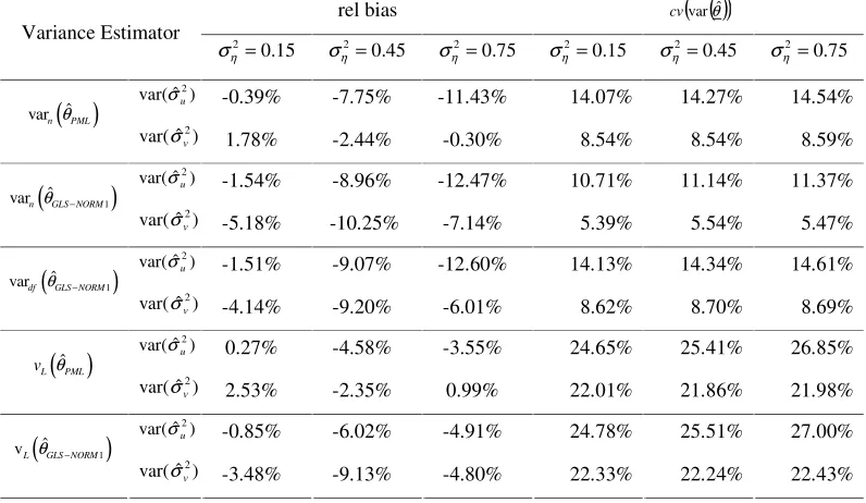
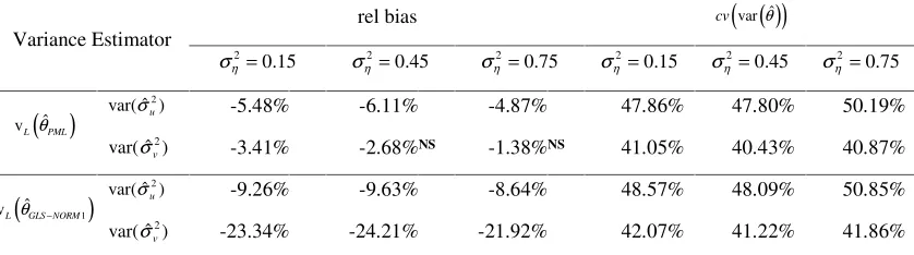
Both methods that allow for clustering have improved properties in terms of relative bias, compared to the first three methods. They are still biased downwards, however, corresponding to other findings for linearization variance estimation (Wolter, 1985, Chapter 8; Kott, 1991). Furthermore, these two methods had larger variances than the first three methods, as expected (Kott, 1991; Korn and Graubard, 1995), as a result of the reduced degrees of freedom for variance

estimation. Moreover, the cvs for both v_L

( )

ˆ_PML and v_L

(

ˆ_GLS−NORM1

)

appear to have a slight

tendency of increasing with larger impacts of clustering. This pattern however is not observed for

the first three methods, which seem to have variances which do not vary greatly with 2

η

σ .

Table 5 includes results that were produced when considering _msim =20 _and sim ₌₁₅ j

n , i.e. 300

cases. Under this situation, the linearization variance estimators which allow for the complex sampling again led to noticeable improvements in terms of relative bias when compared to methods that ignored the sampling scheme. The smaller number of sample clusters does, however, seem to have led to some increases in relative bias, although these are still smaller than the cvs. Neither the

relative bias nor the cv were found to vary greatly with 2

η

σ .

Table 6 includes results that were produced when _msim =15 _and sim ₌₁₀ j

n , i.e the number of

SSUs selected per cluster was further reduced, and the sample size was diminished to 150. further increases in relative bias were observed although again the relative biases were smaller than the cvs.

As in Table 5 there was no strong relationship between either the relative bias or the cv with 2

η

σ .

there is a tendency for the variance to be underestimated if the number of sampled clusters is small, say twenty or below.

7. Conclusion

This paper has proposed some methods of making inference about parameters in panel data models, allowing for complex sampling schemes. Methods have been evaluated using a simulation study based upon data from the BHPS. The study indicated that: (i) overall most of the proposed methods perform satisfactorily under clustered designs; (ii) ADF methods do not always perform as we expected, although often these had the smallest variance, were generally less sensitive to clustering, and had the best performance for stronger departures from normality; and (iii) ML and PML estimators produced satisfactory performance in terms of bias and variance, even when the normality assumption was violated.

Baltagi, B. H. (2001) Econometric Analysis of Panel Data. 2 ed., Chichester, John Wiley & Sons. Belisle, C. J. P. (1992) Convergence theorems for a class of simulated annealing algorithms on Rd.

Journal of Applied Probability, Vol. 29, 885-895.

Bentler, P. M. and Weeks, D. G. (1980) Linear Structural Equations with Latent Variables.

Psychometrika, Vol. 45, N. 3, 289-308.

Berrington, A. (2002) Exploring Relationships Between Entry Into parenthood and Gender Role Attitudes: Evidence from the British Household Panel Study. In Lesthaeghe, R. ed Meaning and Choice: Value Orientations and Life Course Decisions. Brussels, NIDI.

Binder, D. A. (1983) On the Variances of Asymptotically Normal Estimators from Complex Surveys. International Statistical Review, 51, 279-292.

Bollen, K. A. (1989) Structural Equations with Latent Variables. New York, John Wiley & Sons. Brewer, K. R. W. and Mellor, R. W. (1973) The effect of sample structure on analytical surveys.

Australian Journal of Statistics, 15, 145-52.

Browne, M. W. (1977) Generalized Least-Squares Estimators in the Analysis of Covariance Structures. In Aigner, D. J. and Goldberger, A. S. eds. Latent Variables in Socio-Economic Models. Amsterdam, North-Holland.

Browne, M. W. (1982) Covariance Structures. In Hawkins, D. M. eds. Topics in Applied Multivariate Analysis. Cambridge, Cambridge University Press.

Browne, M. W. (1984) Asymptotically distribution-free methods for the analysis of covariance structures. British Journal of Mathematical and Statistical Psychology, 37, 62-83.

Byrd, R. H., Lu, P., Nocedal, J. and Zhu, C. (1995) A limited memory algorithm for bound constrained optimization. Journal of Scientific Computing, Vol. 16, 1190-1208.

Chambers, R. L. and Skinner, C. J. eds. (2003) Analysis of Survey Data. Chichester, John Wiley & Sons.

Diggle, P. J., Heagerty, P., Liang, K. & Zeger, S. L. (2002) Analysis of Longitudinal Data. 2nd _ed. Oxford, Oxford University Press.

DuMouchel, W. H. and Duncan, G. J. (1983) Using survey weights in multiple regression analysis of stratified samples. Journal of the American Statistical Association, 78, 535-43.

Fan, P. -L. and Marini, M. M. (2000) Influences on gender-role attitudes during the transition to adulthood. Social Science Research, Vol. 29, 258-283.

Feder, M., Nathan, G. and Pfeffermann, D. (2000) Multilevel Modelling of Complex Survey Longitudinal Data with Time Varying Random Effects. Survey Methodology, Vol. 26, N. 1, 53-65.

Fletcher, R. and Reeves, C. M. (1964) Function minimization by conjugate gradients. Computer Journal. Vol. 7, 148-154.

Fuller, W. A. (1975) Regression Analysis for Sample Surveys. Sankhya. Vol. 37, Series C, 117-132. Fuller, W. A. (1987) Measurement Error Models. New York, John Wiley & Sons.

Holt, D., Smith, T. M. F. and Winter, P. D. (1980) Regression analysis of data from complex surveys. Journal of the Royal Statistical Society, Series A, 13, 303-20.

Hsiao, C. (2003) Analysis of Panel Data. 2nd ed. Cambridge, Cambridge University Press.

Isaki, C. T. and Fuller, W. A. (1982) Survey Design Under the Regression Superpopulation Model.

Journal of the American Statistical Association. Vol. 77, n. 377, 89-96.

Jones, R. H. (1993) Longitudinal Data with Serial Correlation: A State-space Approach. London, Chapman and Hall.

Jöreskog, K. G. (1970) A General Method for Analysis of Covariance Structures. Biometrika, Vol. 57, N. 2, 239-251.

Jöreskog, K. G. and Goldberger, A. S. (1972) Factor Analysis by Generalized Least Squares.

Kalton, G. and Brick, M. (2000) Weighting in household panel surveys. In Rose, D. ed.

Researching Social and Economic Change: the Uses of Household Panel Studies. London, Routledge.

Kish, L. and Frankel, M. R. (1974) Inference from Complex Samples. Journal of the Royal Statistical Society – Series B, Vol. 36, N. 1, 1-37.

Konijn, H. S. (1962) Regression analysis in sample surveys. Journal of the American Statistical Association, 57, 590-606.

Korn, E. L. and Graubard, B. I. (1995) Analysis of Large Health Surveys: Accounting for the Sampling Design. Journal of the Royal Statistical Society – Series A, Vol. 158, N. 2, 263-295. Kott, P. S. (1991) A Model-Based Look at Linear Regression with Survey Data. The American

Statistician, Vol. 45, N. 2, 107-112.

Liang, K. and Zeger, S. L. (1986) Longitudinal Data Analysis Using Generalised Linear Models.

Biometrika, Vol. 73, n. 1, 13-22.

McDonald, R. P. (1980) A Simple Comprehensive Model for the Analysis of Covariance Structures: Some Remarks on Applications. British Journal of Mathematical and Statistical Psychology, Vol. 33, 161-183.

Müthén, B. O. and Satorra, A. (1995) Complex Sample Data in Structural Equation Modelling.

Sociological Methodology, Vol. 25, 267-316.

Nelder, J. A. and Mead, R. (1965) A simplex algorithm for function minimization. Computer Journal, Vol. 7, 308-313.

Nocedal, J. and Wright, S. J. (1999) Numerical Optimization. New York, Springer.

Pfefferman, D., Skinner, C. J., Holmes, D. J., Goldstein, H., & Rashash, J. (1998). Weighting for unequal selection probabilities in multilevel models. Journal of the Royal Statistical Society,60, 23–40.

Pourahmadi, M. (1999) Joint Mean-covariance with Applications to Longitudinal Data: Unconstrained Parameterisation. Biometrika, Vol. 86, n. 3, 677-690.

Satorra, A. (1992) Asymptotic Robust Inferences in the Analysis of Mean and Covariance Structures. Sociological Methodology, Vol. 22, p. 249-278.

Satorra, A. and Bentler, P. M. (1986) Some Robustness Properties of Goodness of Fit Statistics in Covariance Structure Analysis. Proceedings of the Business and Economics Statistics Section, p. 549-554, Alexandria, VA: American Statistical Association.

Scott, A. J. and Holt, D. (1982) The effect of two-stage sampling on ordinary lest-squares methods.

Journal of the American Statistical Association, Vol. 77, 848-854.

Shah, B. V., Barnwell, B. G., and Bieler, G. S. (1997) SUDAAN User’ Manual, Release 7.5. vol. 1 e 2, Research Triangle Park, NC: Research Triangle Institute.

Shah, B. V., Folsom, R. E., LaVange, L. M., Wheeless, S. C., Boyle, K. E., and Williams, R. L. (1995) Statistical Methods and Mathematical Algorithms Used in SUDAAN. Research Triangle Park, NC: Research Triangle Institute.

Shah,B.V.,Holt,M.M.&Folsom,R.E.(1977)InferenceAboutRegressionModels fromSample SurveyData.Bulletinof the International Statistical Institute, 47(3), p. 43-57.

Skinner, C. J. (1989) Domain Means, Regression and Multivariate Analysis. In Skinner, C. J., Holt, D. and Smith, T. M. F. eds. Analysis of Complex Surveys. Chichester, John Wiley & Sons. Skinner, C. J. and Holmes, D. (2003) Random Effects Models for Longitudinal Survey Data. In

Skinner, C. J. and Vieira, M. D. T. (2005) Design Effects in the Analysis of Longitudinal Survey

Data. S3RI Methodology Working Papers, M05/13, 23pp, Southampton, Southampton

Statistical Sciences Research Institute.

Sutradhar, B. C. and Kovacevic, M. (2000) Analysing ordinal longitudinal survey data: Generalised estimating equations approach. Biometrika, Vol. 87, N. 4, 837-848.

Swain, A. J. (1975) A Class of Factor Analysis Estimation Procedures with Common Asymptotic Sampling Properties. Psychometrika, Vol. 40, N. 3, 315-335.

Taylor, M. F. ed, with Brice J., Buck, N. and Prentice-Lane E. (2001) British Household Panel Survey - User Manual - Volume A: Introduction, Technical Report and Appendices. Colchester, University of Essex.

Ware, J. H. (1985) Linear Models for the Analysis of Longitudinal Studies. The American Statistician, Vol. 39, N. 2, 95-101.

Wolter, K. M. (1985) Introduction to Variance Estimation. New York, Springer.

Woodruff, R. S. (1971) A Simple Method for Approximating the Variance of a Complicated Estimate. Journal of the American Statistical Association, Vol. 66, N. 334, 411-414.

Wooldridge, J. M. (2001) Econometric Analysis of Cross Section and Panel Data. 1st _ed.

Cambridge, MA, MIT Press.

Yuan, K-H. and Bentler, P. M. (1997) Improving Parameter Tests in Covariance Structure Analysis.

100

=

n n=200 n=500 n=1340

Estimator

rel bias cv rel bias cv rel bias cv rel bias cv

2

ˆu

σ -16.76% 17.77% -9.21% 12.14% -3.40% 7.16% -1.42% 4.29%

1

ˆ

GLS NORM

θ − ₂

ˆv

σ -9.70% 8.41% -4.68% 5.56% -1.74% 3.39% -0.74% 1.90%

2

ˆu

σ -6.43% 17.69% -3.77% 11.77% -1.18% 7.12% -0.60% 4.27%

2 ˆ GLS NORM θ ₋ 2 ˆv

σ 6.41% 7.19% 3.51% 5.20% 1.59% 3.27% 0.47% 1.88%

2

ˆ_u

σ -15.79% 19.44% -9.23% 12.76% -3.41% 7.19% -1.46% 4.33% ˆ

GLS L

θ − ₂

ˆv

σ -9.89% 9.04% -4.60% 5.83% -1.72% 3.44% -0.74% 1.93%

2

ˆ_u

σ -9.94% 17.18% -5.61% 11.68% -1.92% 7.08% -0.88% 4.26% ˆ

PML

θ

2

ˆv

[image:28.612.92.538.67.250.2]

σ 0.89% 6.84% 0.74% 5.09% 0.47% 3.25% 0.06% 1.87%

Table 1 – Properties of point estimators when both fitted model and true model are UCM.

100

=

n n=200 n=500 n=1340

Estimator

rel bias cv rel bias cv rel bias cv rel bias cv

2

ˆu

σ -16.73% 29.27% -8.75% 22.07% -4.05% 12.10% -1.63% 7.54%

1

ˆ

GLS NORM

θ − ₂

ˆv

σ -12.30% 10.98% -7.13% 8.08% -2.65% 5.23% -1.02% 3.28%

2

ˆu

σ -7.11% 29.26% -3.32% 22.28% -1.78% 12.17% -0.76% 7.53%

2

ˆ

GLS NORM

θ _{− 2}

ˆv

σ 9.45% 14.00% 4.83% 9.92% 2.18% 6.08% 0.92% 3.66%

2

ˆu

σ -21.82% 29.11% -13.00% 18.55% -6.16% 11.72% -2.56% 7.44% ˆ

GLS L

θ ₋

2

ˆv

σ -17.18% 11.74% -11.54% 8.23% -5.58% 5.16% -2.75% 3.21%

2

ˆu

σ -10.33% 28.91% -5.16% 22.00% -2.54% 12.10% -1.05% 7.53% ˆ_PML

θ

2

ˆv

σ 1.56% 10.84% 0.62% 8.62% 0.51% 5.55% 0.26% 3.47%

Table 2 – Properties of point estimators when fitted model is UCM and true model is UCM-C with t distributed errors

[image:28.612.90.535.322.507.2]

Estimator UCM model AR1 model

2

ˆu

σ 1.44 1.46

2

ˆv

σ _{0.89 0.93}

ˆ_ULS

θ

γˆ - 1.01

2

ˆ_u

σ _{1.27 1.27}

2

ˆv

σ 0.93 0.92

1

ˆ

GLS NORM

θ −

γˆ _{- 1.01}

2

ˆu

σ _{1.52 1.53}

2

ˆv

σ _{0.95 1.06}

2

ˆ

GLS NORM

θ −

γˆ - 1.10

2

ˆu

σ 1.22 1.23

2

ˆv

σ 0.86 0.89

ˆ

GLS L

θ −

γˆ _{- 0.82}

2

ˆ_u

σ _{1.44 1.45}

2

ˆ_v

σ 0.89 0.99

ˆ PML

θ

γˆ _{- 1.04}

Table 3 – Ratios of MSEs of estimators with data generated from UCM-C model (numerator) and from UCM model (denominator) (n=100 and t-distributed errors).

rel bias _cv

( )

_var

( )

θˆ

Variance Estimator 15 . 0 2₌ η

σ 2₌0.45

η

σ 2₌0.75

η

σ 2₌0.15

η

σ 2₌0.45

η

σ 2₌0.75

η σ ) ˆ var( 2 u

σ _{-0.39% -7.75% -11.43% 14.07% 14.27% 14.54%}

( )

ˆ varn θPML

) ˆ var( 2

v

σ 1.78% -2.44% -0.30% 8.54% 8.54% 8.59%

) ˆ var( 2

u

σ -1.54% -8.96% -12.47% 10.71% 11.14% 11.37%

(

ˆ 1

)

varn θGLS NORM−

) ˆ var( 2

v

σ _{-5.18% -10.25% -7.14% 5.39% 5.54% 5.47%}

) ˆ var( 2

u

σ _{-1.51% -9.07% -12.60% 14.13% 14.34% 14.61%}

(

ˆ 1

)

vardf θGLS NORM−

) ˆ var( 2

v

σ -4.14% -9.20% -6.01% 8.62% 8.70% 8.69%

) ˆ var( 2

u

σ _0.27% -4.58% -3.55% 24.65% 25.41% 26.85%

( )

ˆ

L PML v θ ) ˆ var( 2 v

σ _{2.53% -2.35% 0.99% 22.01% 21.86% 21.98%}

) ˆ var( 2

u

σ -0.85% -6.02% -4.91% 24.78% 25.51% 27.00%

(

ˆ 1

)

vL θGLS NORM−

) ˆ var( 2

v

[image:29.612.88.486.445.676.2]

σ _{-3.48% -9.13% -4.80% 22.33% 22.24% 22.43%}

rel bias _cv

(

_var

( )

_θˆ

)

Variance Estimator 15 . 0 2₌ η

σ 2₌0.45

η

σ 2₌0.75

η

σ 2₌0.15

η

σ 2₌0.45

η

σ 2₌0.75

η σ ) ˆ var( 2 u

σ -5.17% -5.25% -4.69% 38.07% 39.03% 40.75%

( )

ˆ

vL θPML

) ˆ var( 2

v

σ -1.54% -0.69% -0.49% 33.55% 33.79% 34.44%

) ˆ var( 2

u

σ -7.31% -7.60% -6.55% 38.42% 39.17% 40.83%

(

ˆ 1

)

vLθGLS NORM−

) ˆ var( 2

v

σ -14.17% -12.87% -12.23% 34.26% 34.39% 35.00%

Table 5 – Properties of variance estimators, when UCM is fitted model, UCM-C is true model, 20

=

sim

m and sim =15

j

n .

rel bias _cv

(

_var

( )

_θˆ

)

Variance Estimator 15 . 0 2₌ η

σ 2₌0.45

η

σ 2₌0.75

η

σ 2₌0.15

η

σ 2₌0.45

η

σ 2₌0.75

η σ ) ˆ var( 2 u

σ -5.48% -6.11% -4.87% 47.86% 47.80% 50.19%

( )

ˆ vL θPML

) ˆ var( 2

v

σ -3.41% -2.68%NS _-1.38%NS _{41.05% 40.43% 40.87%}

) ˆ var( 2

u

σ -9.26% -9.63% -8.64% 48.57% 48.09% 50.85%

(

ˆ 1

)

vLθGLS NORM−

) ˆ var( 2

v

[image:30.612.82.501.267.384.2]

σ -23.34% -24.21% -21.92% 42.07% 41.22% 41.86%

Table 6 – Properties of variance estimators, when UCM is fitted model, UCM-C is true model, _msim =15 _and 10

=

sim j