PhD Dissertation
International Doctorate School in Information and Communication Technologies
University of Trento
Advanced methods for the analysis of
multispectral and multitemporal remote sensing
images
Massimo Zanetti
Advisor:
Prof. Lorenzo Bruzzone
Universit`a degli Studi di Trento
Abstract
The increasing availability of new generation remote sensing satellite multispectral images provides an unprecedented source of information for Earth observation and monitoring. Multispectral images can be now collected at high resolution covering (almost) all land sur-faces with extremely short revisit time (up to a few days), making it possible the mapping of global changes. Extracting useful information from such huge amount of data requires a systematic use of automatic techiques in almost all applicative contexts. In some cases, the strict application requirements force the pratictioner to develop strongly data-driven approaches in the development of the processing chain. As a consequence, the exact rela-tionship between the theoretical models adopted and the physical meaning of the solutions is sometimes hidden in the data analysis techniques, or not clear at all. Altough this is not a limitation for the success of the application itself, it makes however difficult to trans-fer the knowledge learned from one specific problem to another. In this thesis we mainly focus on this aspect and we propose a general mathematical framework for the represen-tation and analysis of multispectral images. The proposed models are then used in the applicative context of change detection. Here, the generality of the proposed models allows us to both: (1) provide a mathematical explanation of already existing methodologies for change detection, and (2) extend them to more general cases for addressing problems of increasing complexity. Typical spatial/spectral properties of last generation multispectral images emphasize the need of having more flexible models to image representation. In fact, classical methods to change detection that have worked well on previous generations of multispectral images provide sub-optimal results due to their poor capability of modeling all the complex spectral/spatial detail available in last generation products. The theoretical models presented in this thesis are aimed at giving more degrees of freedom in the repre-sentation of the images. The effectiveness of the proposed novel approaches and related techniques is demonstrated on several experiments involving both synthetic datasets and real multispectral images. Here, the improved flexibility of the models adopted allows for a better representation of the data and is always followed by a substantial improvement of the change detection performance.
Contents
1 Introduction 1
1.1 Background on optical imagery in remote sensing . . . 1
1.2 Motivation of the thesis . . . 4
1.3 Objectives of the thesis . . . 6
I Novel techniques for numerical minimization of variational functionals for image approximation 11 2 Background 13 2.1 An optical image model . . . 13
2.2 Mathematical methods to image approximation . . . 14
2.3 Challenges and novel contributions . . . 20
3 Numerical minimization of a variational functional to image approxima-tion 23 3.1 Introduction . . . 23
3.2 Numerical minimization of the Blake-Zisserman functional . . . 29
3.3 Numerical results . . . 37
3.4 Conclusions . . . 54
4 Variational approximation of vector-valued images and curves 59 4.1 Introduction . . . 59
4.2 The Blake-Zisserman model for the approximation of vector-valued images and curves . . . 62
4.3 Experimental results: piecewise linear approximation of vector-valued images 69 4.4 Experimental results: polygonal approximation of planar closed curves . . 80
4.5 Conclusions . . . 83
5 Background 89
5.1 Overview of the change detection problem . . . 89
5.2 Change detection methods for multispectral images . . . 91
5.3 Challenges and novel contributions . . . 94
6 The Rayleigh-Rice mixture model for binary change detection 97 6.1 Introduction . . . 98
6.2 A problem of binary change detection . . . 100
6.3 The EM algorithm for parameter estimation of the Rayleigh-Rice mixture density . . . 103
6.4 Experimental results on multispectral images . . . 110
6.5 Conclusions . . . 118
6.6 Acknowledgments . . . 121
6.A Appendices . . . 121
7 A compound multi-class mixture model for change detection 127 7.1 Introduction . . . 128
7.2 Statistical study of the difference image . . . 130
7.3 Derivation of a method for binary decision based on the difference mixture model . . . 135
7.4 Experimental results . . . 143
7.5 Discussion and conclusion . . . 149
7.A Appendices . . . 152
8 A class-wise spatial-contextual approach based on a free discontinuity model for change detection in multispectral images 155 8.1 Introduction . . . 155
8.2 A spatial-contextual framework for class-wise statistical reduction of mul-tispectral images . . . 156
8.3 Binary change detection based on class-wise statistical reduction . . . 160
8.4 Experimental results . . . 161
8.5 Conclusion . . . 165
9 Conclusions and future developments 169 9.1 Conclusions . . . 169
9.2 Future developments . . . 171
Bibliography 173
List of Tables
1.1 Relevant spaceborne multispectral sensors operating from the early eighties to nowadays. First group decommissioned. Second group ongoing missions. 3
3.1 Outer/inner iterations and execution time (seconds) observed in the run of the proposed algorithms. . . 41
3.2 Accuracy in the approximations given by the GS, BCDA and BCDAc with respect to the ideal solution for the considered datasets. . . 43
4.1 Outer(k)/inner(iter) iterations and execution time observed in the mini-mization of the three functional models. . . 76
4.2 Estimation of additive Gaussian noise variance in color images using the MS and the BZred models. . . 80
6.1 Classification error in a two-class decision problem. ωn unchanged pixels,
ωc changed pixels . . . 103
6.2 Iteration details of the proposed EM algorithm on Rayleigh-Rice mixtures with parameters α= 0.4,b = 1, σ= 1 and for different values of ν. . . 109
6.3 Iterations details of the proposed EM algorithm on Rayleigh-Rice mixtures with parameters α= 0.4,b = 1, σ= 2 and for different values of ν. . . 109
6.4 Parameter estimation via EM algorithm and data fitting evaluation for the three considered mixture densities. . . 116
6.5 Performance of change detection based on the thresholding of the magni-tude image for different values of the threshold. . . 119
7.1 EM algorithm iteration details and parameter estimations for both the cosidered mixtures. . . 148
7.2 Comparison of the change detection performance of the method in [1] and the proposed method with respect to optimal performance. . . 150
difference images using channels 5 and 6. The change class contains the fire, the unchange class all the rest. . . 164 8.2 Change detection performance of the Rayleigh-Rice binary detector (rR)
and optimal (opt) performance in the case of the original difference image d (see [1]) and the statistically reduced difference image d. MA, FA and OE are missed alarms, false alarms and overall errors, respectively. . . 167
List of Figures
1.1 Spectral and spatial properties of Landsat, SPOT and Sentinel-2 multi-spectral imagery, [2]. . . 4
1.2 A fire occurred in Sardinia Island (Italy) between August 7-9, 2013 (the total extention of the event is approximately 2400 hectars): (a) environ-mental image of the event, the village on the left is Laconi; (b) false color image of the area affected by the fire composed by three spectral bands of a Landsat 8 image of the scene, spatial resolution is 30 m. . . 5
2.1 A typical optical imaging system, [3]. . . 14
2.2 An example of scale-space representation via the Mumford-Shah piecewise smooth approximation. (a) The original image g is a portion of QuickBird image representing an urban area in Reggio Emilia, Italy. (b) Piecewise smooth approximation u of the image. Functional parameters are selected to represent the image at scale in which textural details are eliminated but basic shapes of the buildings are preserved. (c) map of the detected edges K. 19
2.3 Example of a cartooned image. (a) is the original image g, (b) is the approximation u (the cartoon) obtained via Mumford-Shah piecewise con-stant approximation. (c) is the set of edges K. . . 20
3.1 Limitation of the MS model of detecting second-order geometrical features. (a,b) Gray-scale image with second-order edges. (c) Edge-detection via Mumford-Shah functional compared to (d) a full theoretical exact detection of 2nd-order features. . . 26
3.2 Slice section of the discontinuity set S and its approximation via the re-covering function σ realizing the Γ-convergence. . . 28
3.3 Datasets of the experiment including three gray-scale images and a digital surface model obtained from airborne LiDAR points acquired over Trento, Italy. . . 39
BCDA and BCDAc. Algorithms are stopped by criterion (3.22) with tol-erance T OLF = 10−3. . . 42
3.5 Results of the BCDA method for the considered datasets. First column is the smooth approximation u, second column is the edge-map s and third column is the edge/crease-map z. . . 44 3.6 Particulars of the segmentation for the dataset pearl. . . 45
3.7 Particulars of the segmentation for the dataset airport. . . 46
3.8 Particulars of the segmentation for the dataset barracks. Above, there are the 3D renderings of the surface modelg and its smooth approximation u. In the bottom, there are the edge map sand the edge+crease map z. . . . 47 3.9 Smoothing on synthetic images with different noise levels, image size is
100×100. Row 1: input noisy images g. Row 2: difference g−u. Row 3: edge-detection functions s. Row 4: edge/crease-detection functionsz. . . . 49 3.10 Performance details of BCDA by varying µ and for different variances of
the noise. Test images are 1000×1000 pixels compositions of the pyramidal elements showed in Figure 3.9. For each value ofµwe plot (a) the execution time, (b) the total number, and (c) the average number of iterations of the PCG solver related to u. . . 50 3.11 Performance of BCDA with Diagonal (D) and Block-Diagonal (BD)
pre-conditioners for the PCG solver related to u, versus the size of g. We plot (a) the execution time, (b) the total number, and (c) the average number of iterations of the PCG solver related to u. . . 51 3.12 Test images. (a) Image with jump of variable height h. (b) Image with
a crease of variable slope θ. The slices of functions s,z plotted in Figures 3.13 and 3.14 are located in correspondence of the red dashed lines. . . 53
3.13 Slices of functions s and z obtained by minimizing F in the case of test
image with a jump (Figure 3.12a) for different values of (a,b) and h (c,d). 55
3.14 Slices of functions s and z obtained by minimizing F in the case of test
image with a gradient discontinuity (Figure 3.12b) for different values of (a,b) and tan(θ) (c,d). . . 56
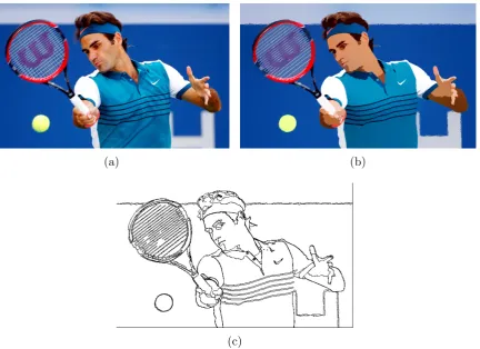
4.1 Craquelure removal via MS and BZ approaches. (a) The input color image represents a portion of the oil painting Girl with a pearl earring. Its ap-proximations are obtained by the three different models: (b) AT-MS, (c)
AFM-BZap, (d) AFM-BZ. . . 72
4.2 Discontinuity functions computed for the three functional models. (a) AT-MS, (b,c)AFM-BZap, (d)AFM-BZ. White corresponds to 1 and black to 0, gray values are in between. . . 73
4.3 Particular of the approximations by zooming the area in the red square in Figure 4.1. (a) Original image, and the results for: (b) AT-MS, (c)
AFM-BZap, (d) AFM-BZ. Notice the over-segmentation effect in (b,c). 74 4.4 Pixel scatterplots of the image portions represented in Figure 4.3. (a)
Original image, (b) AT-MS, (c) AFM-BZap, (d) AFM-BZ. . . 75 4.5 Energy-versus-time at each outer iteration for the three functional
mini-mization cases: (a) AT-MS, (b) AFM-BZap, (c) AFM-BZ. The plots illustrate the descent of each additive term in the functional models. The black dashed line is the total energy. Blue is the Hessian component and Cyan is the AT component associated to the Hessian (present only in
AFM-BZap and AFM-BZ). Red is the gradient component and Ma-genta is the AT component associated to the gradient (present only in
AT-MS and AFM-BZap). Green is the distance term. . . 77 4.6 Estimation of Gaussian additive noise in color image containg challenging
geomteries. (a) Synthetic noise-free generated image, (b) noisy image. Re-constructions of the noisy image are obtained by the (c) AT-MS model, (d) AFM-BZ model. Particulars zoomed at the crack-tip end for the (e)
AT-MS solution (white traits emphasize the main directions of the dis-continuity edges) and the (f) AFM-BZ solution. . . 79 4.7 Extraction of building edges from DSM. (a) 3d rendering of a DSM
rep-resenting an old barrack. (b) Edge map of the main (U-shaped) building obtained by segmenting the DSM using the BZ model for gray-scale im-ages [4]. The points correspond to the pixels where the functions(the edge detection function) is 0. . . 81
4.8 Curve approximation results obtained for different parameter choices of the CSSP model. The range of values used in the experiments allowed us to explore the behaviour of the solution from over- to under- fitting. No gradient discontinuity is allowed by the model. . . 83
4.9 Curve approximation results obtained for different parameter choices of the BZmodel. The range of values used in the experiments allowed us to explore the behaviour of the solution from under- to over- fitting passing also through polygonal solutions. The best polygonal approximation is (i), i.e., for parameters λ= 10−5 and ν = 10−4. . . . 84
change detection procedure. . . 90
6.1 Geometrical interpretation of the posterior probability thatxoriginated in the h-th component given Ψ0, as p (ωh|x,Ψ0) =Ch/(C1+C2) for h= 1,2. . 105 6.2 Histograms of samplesxgenerated from p (ρ|Ψ) withα = 0.4,b = 1,σ = 1
and for different values of ν. . . 110
6.3 Histograms of samplesxgenerated from p (ρ|Ψ) withα = 0.4,b = 1,σ = 2 and for different values of ν. . . 110
6.4 Dataset A. Synthetic two-band difference image. (a) Magnitude of the difference image, (b) map of simulated changed pixels (black). . . 112
6.5 Dataset B: images of Lake Mulargia (Italy) acquired by the Thematic Map-per sensor of the Landsat 5 satellite: (a) channel 4 of the image acquired in September 1995; (b) channel 4 of the image acquired in July 1996; (c) change reference map indicating the enlargement of the lake (black) and an open quarry (red). . . 113
6.6 Dataset C: images of Lake Omodeo and surrounding area (Italy) acquired by the Operational Land Imager sensor of the Landsat 8 satellite: (a) channel 5 of the image acquired in July 2013; (b) channel 5 of the image acquired in August 2013; (c) change reference map indicating the burned area extension (black) and other minor changes related to clouds and water (red). . . 114
6.7 Histograms of the magnitude of the difference image and plot of the esti-mated densities. . . 117
6.8 Change detection maps obtained by thresholding the magnitude image us-ing TRR (a,d,g), TGG (b,e,h) and TM OE (c,f,i). In black are the estimated
changed pixels Wc, in white the estimated unchanged pixels Wn. . . 120
7.1 Example of statistical dependency of the difference image with respect to the input pair when the number of natural classes isC= 2. (a) The natural class φ2 is only observable in image y2, thus the resulting difference image has only one unchange behaviour ω1 and one change behaviour ω12 (from class φ1 to φ2). (b) Both natural classes φ1, φ2 are observable in the two images. Therefore, they have their own unchange statistical behaviours ω1, ω2, and mutual change behaviours ω12 (from class φ1 to φ2), and ω21 (from class φ2 toφ1). . . 134
7.2 Illustration of the datasets analyzed in the experiments. Thep pictures show pre and post images in one band and a reference map of the changes (red pixels are minor changes with respect to the main changes that are respresented by black pixels) for (a,b,c) dataset A, (d,e,f) dataset B, (g,h,i) dataset C, and (j,k,l) dataset D. . . 146 7.3 Fitting capability of the considered methods. Estimated densities are
su-perimposed to the histograms of the magnitude samples. In the legends also the distance metrics between the estimated densities and the histograms are given. . . 147 7.4 Change detection map obtained on (a,b) dataset A, (c,d) dataset B, (e,f)
dataset C, and (g,h) dataset D. Blue pixels are missed alarms, red ones are false alarms and green ones are correctly detected changes. . . 151
8.1 The proposed tiling scheme with related size parameters. . . 159 8.2 Hitograms of the differences between the solutions. x-axis (binned
differ-ence values) is restricted to a portion where more than 99,99% of pixels are counted. The central bars are cutted at the top. . . 162 8.3 A portion of the difference u−ut and of the function zt in correspondence
of a cross tile junction (indicated by the red traits). The scene represents some old barracks and sourrounding area. . . 162 8.4 Landsat 8 dataset used in the experiments. (a) Original difference image
(false color composition), see [1]. (b) Reference map of the changes. Black pixels belong to the fire, the red ones are minor changes unrelated to the fire. (c) Difference image after statistical reduction (false color composi-tion), this image is used for computations in the experiments. (d) Map of the class boundaries extracted from the reduced image. The false color compositions are obtained by putting channels 3,5,6 of the Landsat image into R,G,B. . . 164 8.5 Histogram of the magnitude of the statistically reduced difference image
and estimated density. Notice that the two classes are well separated. . . . 165 8.6 Results of the change detection. (a) CD map obtained with the
Rayeligh-Rice binay detector (rR) applied to the reduced image, (b) CD map related to the optimal threshold (opt) applied to the reduced image. For compar-ison with the methods proposed in the two previous chapters: (c) CD map obtained with the rR binary detector (Chapter 6) applied to the image before reduction, and (d) CD map obtained with the rrRbinary detector (Chapter 7) applied to the image before reduction. In all CD maps red, blue and green are false alarms, missed alarms and hits, respectively. . . . 166
Chapter 1
Introduction
This chapter gives an overview of the role played by multispectral imagery in remote sensing with its applications, it describes the main motivations and the objectives of the thesis and presents the whole structure and organization of the document. This dissertation is divided into two main parts; the content of each part is described more in detail in each corresponding introductive section.
1.1
Background on optical imagery in remote sensing
Remote Sensing (RS) encompasses a variety of technologies and techniques to continu-ously observe the Earth surface by means of sensors mounted on aircraft or spacecraft platforms. The peculiarity of RS is that certain properties of real objects can be measured remotely without relying on physical contact. This makes RS an essential tool for the study of ours planet evolution. Indeed, it is already widely employed in different appli-cation domains such as forestry, agriculture, urban management, oceanography, natural disaster monitoring, etc.
at VHR typically records the radiation in the red, green and blue (RGB) regions of the visible range (from 390 to 700 nm), in the near-infrared (NIR) region (from 700 to 900 nm) and possibly in the short-wave infrared (SWIR) region (from 1100 to 3000nm). Geo-metrical resolution of satellite VHR images ranges between 2 and 5 meters. Multispectral sensors at moderate resolution (from 10 to hundreds of meters) are able to record the radiation in the visible and NIR ranges (in shorter intervals) but they can also measure farther portions of the spectrum covering the middle-infrared (MIR) and far-infrared (FIR or thermal) regions. Hyperspectral sensors sample over several (from tens to hundreds) narrow contiguous portions of the spectrum. These four types of optical images present complementary features, they have their own advantages and disadvantages and they can serve at different purposes in various applicative contexts. One particular feature that makes MS imagery very attractive for global studies is that MS sensors typically have large swaths (up to two or three hundreds of kilometers). Therefore, images can be col-lected at global scale with shorter revisit time, if compared to the others. We report in Table 1.1 specifications of some of the more relevant satellite missions that have been launched with MS sensors mounted on board since the early eighties.
Figure 1.1: Spectral and spatial properties of Landsat, SPOT and Sentinel-2 multispectral imagery, [2].
to be essentially described in statistical terms. Indeed, they show spatial homogeneity and they can be accurately characterized by spectral vectors. In the sequel, these properties are investigated in greater detail. Novel results in the mathematical modeling of multi-spectral images are proposed and applied in the context of change detection. However, the character of the proposed theory is general and can be applied to other contexts as well.
1.2
Motivation of the thesis
Motivation of the thesis 5
(a) (b)
Figure 1.2: A fire occurred in Sardinia Island (Italy) between August 7-9, 2013 (the total extention of the event is approximately 2400 hectars): (a) environmental image of the event, the village on the left is Laconi; (b) false color image of the area affected by the fire composed by three spectral bands of a Landsat 8 image of the scene, spatial resolution is 30m.
for the next generation of operational products such as land-cover maps, land-use change detection maps and geophysical variables. This allows for an accurate monitoring of the land surface changes in wide geographical areas according to both long term (e.g., yearly) and short term (e.g., daily) observations. The detection and understanding of changes occurred at the ground level is essential for studying the global change, the environmental evolution and the anthropic phenomena. For this reason, the development of change-detection techniques for the analysis of multitemporal remotely sensed images is now becoming one of the most important research topics in remote sensing.
the purpose of environmental monitoring it is possible to detect changes in snow coverage, extention or reduction of thematic areas (e.g. forests, deserts, urban areas); in vegetation monitoring and agriculture surveys it is possible to detect vegetation indexes fluctuations, changes in vegetation life conditions, soil moisture variations.
Thanks to the spatial/spectral level of detail available in MS images, it is possible to specifically identify the spectral signature of certain classes and then perform detecting steps aimed at identifying variations in their spectral behaviour. Given its well-recognized importance in terms of applications, CD is a widely covered topic in literature. A huge vastity of models and methods have been proposed to solve as many different problems. However, in most of the cases the methodological development of CD procedures is driven by the problem and often the literature lacks in general models. This fact limits the possiblity of passing and adapting the knowledge learned from certain problems to even slightly different applicative contexts and makes the general understanding of the under-lying physical mechanism more difficult. Another limitation of current state-of-the-art methods is that, many empirical models that has worked well for the first generation of MS imagery show to be inefficient for addressing the new challenges introduced with the last generation products.
1.3
Objectives of the thesis
The aim of this thesis is to propose a general mathematical framework for the repre-sentation and analysis of RS images. If transposed to the applicative context of CD, the proposed models are able to provide both (1) a mathematical explanation of already existing methodologies, and (2) a framework to extend them to more general cases for addressing problems of increasing complexity. In our presentation, the mathematical representation of images as functions plays a central role. Certain assumptions can be made on the function models to let them accurately describe image properties that are of particular interest for the application. We will focus in particular on the description of geometrical and statistical properties of the images. It is a matter of fact that, the full information content present in an image can be completely modeled only in ideal cases. Rather, simplified models of the images are always (explicitly or implicilty) used as a basis for the rationale of most of the image processing techinques. Unfortunately, when these ideal models are not clear to the pratictioner, it is difficult to interpret in a meaningful and reasonable way the results obtained after processing.
Objectives of the thesis 7
statistical models for change detection in multispectal images (Part II of this thesis). In the following, we describe how the thesis presentation is structured, by focusing in particular on the main challenges and the innovative contributions introduced in the PhD activity.
1.3.1 Part I
The first part of the thesis is mainly concerned with image approximation based on vari-ational methods. The varivari-ational approach provides a way to return an approximation of an image which is a composition of several pieces on which the image values are homo-geneous in terms of derivatives. According to the derivative order that is penalized, we have first-order and second-order variational models to image approximation. Two well-known variational models to image approximation from computer vision due to Mumford and Shah [3] and Blake and Zisserman [5] are investigated. Given the large (almost in-explored) potential of variational methods to the processing of MS images, we have put a lot of effort in the study and the application of image approximation models in the remote sensing context. The RS highlights some well-known drawbacks of mathematical methods to image processing: the difficult scalability to large sized data and the extension of already existing models from their native scalar version (in which they are originally formulated) to the vector-valued case. An extensive study in this direction is proposed.
Chapter 2. In this chapter mathematical methods to image approximation are pre-sented, with particular emphasis on variational methods and their applications. The chapter also introduces to the content of the first part of the thesis and describes the novel contributions.
Chapter 3. In this chapter we propose a novel approach to the numerical minimization of variational functionals with free-discontinuities that relies on a compact matricial formulation and an efficient iterative solver. In our exposition we take advantage of an extended formulation of the Mumford-Shah variational functional depending also on second-order derivatives due to Blake and Zisserman. Several experiments on both synthetic and real images are presented to demonstrate the various capabilities of variational models to provide simplified approximations of images.
numerical approach to minimization is extended to the case of vector-valued inputs. The proposed method is then applied to difficult problems of image restoration and boundary approximation.
1.3.2 Part II
In the second part of this thesis we mainly investigate the statistical properties of mul-tispectral images with special focus on the analysis of multitemporal images for CD. Very often RS images are modeled as realizations of a set of random variables following a specific statistical distribution. However, in some cases the statistical models associ-ated to the images are not flexible enough to allow a precise description of them. As a consequence, some methodologies that rely on too simple statistical models may give in-accurate results. In the thesis we introduce some new statistical models to the description of the distribution of spectral difference-vectors and we derive from them novel methods to change detection based on image differencing. Differently to what is typically done in the literature, we do not rely on a-priori assumptions on the difference image. Instead, we weaken this constraint and propose a theoretical study by showing that the statistical description of the difference image can be derived from general assumptions on the single time images. By taking advantage of these general models, we further study the statis-tical distribution of the change vectors when coordinates are changed to magnitude and we devise efficient numerical algorithms for the binary detection of changes in bitemporal MS images that overcome the performance of typical empirical approaches.
Chapter 5. This chapter presents an overview of the change detection problem in remote sensing and the methods proposed in literature to address it on multispectral images. The chapter also includes a more detailed description of the contributions of this thesis with respect to the state-of-the-art.
Chapter 6. In this chapter, the standard two-class unchange/change model for binary CD is derived starting from the hypothesis of Gaussian distribution of natural classes in the difference image. When coordinates are changed to magnitude, we show that the two-class model can be described by a Rayleigh-Rice mixture. Parameter estimation of this mixture is a non-trivial task as this model is non-conventional (a typical conventional model which is often used for binary decision is based on a Gaussian mixture). Therefore, we devise a version of the Expectation-Maximization (EM) algorithm which is specifically tailored for the Rayleigh-Rice mixture.
Objectives of the thesis 9
the spectral behaviour of the difference image. Therefore, the intrinsic nature of the unchange/change macro classes is expected to be more complex. This is even more evident in last generation MS images, where the radiometric resolution is sensibly improved and more classes can be represented via their spectral characteristics. To have more chances to better represent last generation data, in this chapter we pro-pose a new compound multiclass model for the CD problem that both extends what is previusly done and also provides a general framework for many CD approaches.
Part I
Novel techniques for numerical
minimization of variational
Chapter 2
Background
This chapter introduces to the content of Part I. Firstly, a mathematical optical image model and the theory of mathematical methods to image approximation are briefly re-viewed and variational models are introduced. In particular, some important properties of free discontinuity models are recalled. Then, the main challenges addressed in this part of the thesis and a description of related contributions are presented.
2.1
An optical image model
The typical function representation of an optical image can be explained in terms of the basic optical acquisition system [3]. The optical device is located in pointP in the 3-D real world and it is pointed towards the subject of the scene, see Figure 2.1. The sensor is able to record the intensity of the light (restricted to a specific interval of the spectrum) coming from the reflective source in radial direction (with centerP). This direction intersects the focal plane in one point, therefore a set of two-dimensional coordinates can be associated to the record of the light intensity. Thus, let us definex∈Ω0 ⊂R2 the spatial coordinate (for convenience restricted to a bounded rectangular region Ω0 of the plane) and g(x) the recorded light intensity at point x. The value g(x) can be either a scalar or a B -dimensional vector depending on the capability of the sensor of recording the spectral response of objects in different intervals of the spectrum (e.g., this is the typical case of multispectral scanners). The functiong(x) : Ω0 →RB is called an image (this is a general notation that also includes the scalar case forB = 1). To better understand what kind of function isg like, one can consider the simple, yet effective, model depicted in Figure 2.1. ObjectsOi that are homogenous in terms of the reflected light intensity and that can be
seen from point P would be imaged to spatially homogenous regions Ωi ⊂ Ω0. Relative position of objectsOi(front, back, partial occlusion) would cause imaged edge boundaries
Figure 2.1: A typical optical imaging system, [3].
expected to be piecewise smooth, i.e., well modeled by a set of smooth functionsgi defined
over disjoint sets Ωi. Of course, this model is ideal as what is observed in real images
is typically more complex: often objects are characterized by textured of fragmented patterns instead of homogeneous patches, shadows would typically result in shallow edges, etc. Noise measurement is another source of deviation from the ideal model. This process of contamination of the ideal image can be formalized by incorporating the physics of the vision mechanism, noise measurement, etc., in a functional transformation Λ that relates the ideal image u to the real recorded g as
g = Λ(u). (2.1)
In general, the trasformation Λ is not explicit, thus the problem of recovering ufromg is an inverse ill-posed problem. The aim of mathematical methods to image approximation is that of recovering a regular approximation u of a real imageg.
2.2
Mathematical methods to image approximation
According to the assumptions that are made on u (and on Λ), there are different ap-proximation approaches. Mathematical methods to image apap-proximation can be mainly divided into two groups: partial differential equation (PDE) methods and variational methods. In the following these two approaches are briefly reviewed.
2.2.1 Partial differential equation methods
Mathematical methods to image approximation 15
formal requirements the image processing transforms must satisfy [7], this model reflects causality, linearity and isometry invariance which are characterizing properties of the heat semi-group. Images at every scale form a family that depend on a temporal parameter t. Each imageu(t, .) of the family satisfyies the partial differential equation (PDE):
∂tu= div [∇u] in R×Ω0, with u(0, .) =g, (2.2) wheregis the input image, a non-negative real-valued function defined over the (rectangu-lar) domain Ω0 ⊂R2. Here the concept of scale-space is strictly related to the parameter
t that determines the width of the Gaussian kernel, i.e. to the amount of noise reduc-tion. Anyway, the model is fully isotropic and does not take into account any structural information of the input image. It blurs out both noise and interesting features of the image such as edges or points of gradient discontinuity. For recovering at this drawback, some modifications of the previous formulation have been proposed. Perona and Malik [8] introduced in formulation (2.2) a term that makes the diffusion anisotropic. More specifi-cally, the diffusion is inhibited according to local properties of the image that are detected by a function c=c(|∇u|) that depends on the gradient. The result is a slighlty changed concept of scale-space that can be formalized by the differential problem
∂tu= div [c(|∇u|)∇u] in R×Ω0, with u(0, .) =g. (2.3) Altough this formulation is general, particularly effective results in enhancing edges have been obtained by usingc(s) = (1 +s2/λ2)−1. Here the positive parameterλ ensures that the diffusion is low when high gradients are detected. A variation on this model have been proposed independently by Rudin and Osher [9]. In particular in their formulation, which is equivalent to the Perona-Malik case where the function c = −1/|∇u|, the resulting PDE represents the flow generated by the minimization of the Total Variation, i.e. the quantity
Z
Ω0
|∇u|dx, (2.4)
with some constraints onu to be fullfilled. In this different view, the variational nature of the denoise-recovering problem becomes more evident.
2.2.2 Variational methods
modification of the PDEs to obtain more and more meaningful solutions becomes a critical step. On the other hand, the real edge-detection step that locates the object boundaries at different scales is still considered as a subsequent and independent step. Diffusion-based methods only enhance edges and do not explicitly provide their detection. In this perspective, the variational approach seems to be more flexible and allows for having a proper and explicit modelization of all the components: smoothing, edge-detection, scale-space representation.
A first-order model: the Mumford-Shah functional
By fully exploiting a variational framework, Mumford and Shah [3] proposed a model for image approximation based on the minimization of the following functional
E(u, K) = Z
Ω0\K
|∇u|2dx+αH1(K) +µ Z
Ω0
|u−g|2dx (2.5)
among all the functions continuously differentiable outside K, i.e. u∈C1(Ω0\K), where K ⊂Ω is compact. Here,H1is the 1-dimensional Hausdorff measure, andα, µare positive parameters. This functional model has several interpetations and specializations that can be formulated depending on specific assumptions/constraints that can be made on u and the other parameters. Hereafter are some examples.
Piecewise smooth approximation. This is the most general case, as defined above. The minimization of the first term in (3.1) forces u to be smooth outside K, which has to be a one-dimensional set with finite length because of the term H1(K). The last distance term forces u to be close to (i.e., an approximation of) the original image g. The unknown set K can be easily understood as the set of the disconti-nuities of u, indeed the minimization of (3.1) is a prototype of free discontinuities problem, [12]. A solution of this formulation would explicitly provide: the set K of the edges, and, u a piecewise smooth version of the original image g. By changing the values of the parameters in (3.1) to augment the noise-reduction effect, different scales are reachable. This fact is enforced in [13], where a strict relationship be-tween the Mumford-Shah and Perona-Malik approaches to segmentation is found. In particular, it is shown how the parameters of the Mumford-Shah functional can be interpreted as parameters regulating an anisotropic diffusion process applied to the image g. An example is shown in Figure 2.2.
Mathematical methods to image approximation 17
• Ωi are open connected sets with smooth boundary ∂Ωi
• let K =∪nΩ
i=1∂Ωi be the total partition boundary, then∪in=1Ω Ωi = Ω0∪K;
• Ωi∩Ωj =∅ for i6=j.
We define the space of piecewise constant functions over the partition Ω to be P C(Ω) := {u : u(x) = ui ∈ R for all x ∈ Ωi}. The functional (3.1) restricted
to this class of functions is
E(u, K) =
nΩ
X
i=1 Z
Ωi
|ui−g|2dx+ν0H1(K) (2.6) as the gradient term vanishes. Fixed Ω, it can be proved that the unique minimizer u∗ of (2.6) is the piecewise function whose values are the integral means of g over the sets Ωi, i.e., u∗i = gΩi := |Ωi1|
R
Ωig dx. Therefore, the minimization of (2.6) is equivalent to the minimization of
E0(K) =
nΩ
X
i=1 Z
Ωi
|g−gΩi|2dx+ν0H1(K) (2.7) which depends on the only variable K. It can be shown that the minimization of E0 is a well-posed problem. If g is continuous there exists a minimizing K made up of a finite number of singular points joined by a finite set of C2-arcs. The resulting piecewise constant functionu∗ obtained by minimizing (2.7) is often called a cartoon
of g, see Figure 2.3.
Markov Random Fields. By changing the representation of the image model from con-tinuous to discrete, it can be shown that the piecewise constant approximation can be derived as a specialization of a Markov Random Field (MRF) model. Con-sider G = (V, E) to be an undirected graph with nodes V = {1, . . . , n} and edges E = {(i, j) ∈ V × V : ifi, j are connected}. To each node i we assign a ran-dom variable vi that takes values on a discrete set A = {a1, . . . , ak} and we call
(G, A) a random field. We denote a possible configuration of the random field by v = (v1, . . . , vn) where eachvi ∈A. If we measure the energy of a configuration v as
U(v) =X
i∈V
G(vi) +ν1 X
i∈V
X
j∈N(i)
F(vi, vj), (2.8)
sensitivity of the random field to external forces (it is often called external interaction function), whereas F describes the energy generated by local inner interactions (it is often called internal interaction function). If the edges of the graph form a reticular structure, the random variables vi can be associated to pixels values of an image u
via the simple assignmentvi =u(xi), wherexi is a spatial discrete coordinate. Given
an image g, by definingG(vi) := [u(xi)−g(xi)]2 and F(vi, vj) := δ(|u(xi)−u(xi)|),
where δis the kronecker function, we get that (2.8) is exactly the discrete version of (2.6) for a suitable choice of the parameter ν1. Notice that, via the kronecker func-tion, the double summation in (2.8) returns a multiple of the length of the interface that separates pixels with different values, i.e., a multiple of the length of K in a discrete setting.
A second-order model: the Blake-Zisserman functional
The Mumford-Shah model assumes the ideal image u approximating g to be essentially piecewise contant. Indeed, the gradient term in the energy penalizes variations of intensity outside a set of finite one-dimensional length, i.e., the set of image discontinuities. This gradient penalization is often called 1st-order penalization as it affects 1st-order deriva-tives of the solution. In some cases, 1st-order penalization is a too strong assumption as some gradients of light intensity are proper characteristics of the image and the piecewise nearly-flat approximation of them might result too coarse. In order to give more flexibility to the approximation model, Blake and Zisserman [5] proposed a 2nd-order penalization variational model to image approximation with the aim of providing a piecewise linear approximation of the image. The model depends on 2nd-order derivatives and allows free discontinuities and free gradient discontinuities and it is based on the minimization of
E(u, K0, K1) = Z
Ω0\(K0∪K1)
|Hu|2dx +µ Z
Ω0
|u−g|2dx +αH1(K
0) +βH1(K1\K0), (2.9)
Mathematical methods to image approximation 19
(a) (b)
(c)
(a) (b)
(c)
Figure 2.3: Example of a cartooned image. (a) is the original image g, (b) is the approximation
u (the cartoon) obtained via Mumford-Shah piecewise constant approximation. (c) is the set of edges K.
2.3
Challenges and novel contributions
This part of the thesis presents novel results for the numerical minimization of variational functionals for image approximation due to Mumford-Shah and Blake-Zisserman. We pro-pose in the following chapters an extensive and detailed presentation of the application of variational methods in different applicative contexts both in the remote sensing (statis-tical reduction of multispectral images, piecewise linear approximation of urban Digital Surface Models) and the image processing (image restoration, polygonal boundary recov-ering) domains. Our main requirements for the implementation of these methods were: (1) obtaining high computational efficiency, (2) dealing with vector-valued images, and, (3) developing highly parallelizable code.
Challenges and novel contributions 21
the variational approximation by Ambrosio, Faina and March (AFM) [14] has some ad-vantages: it is particularly suited for numerical implementation and it allows the explicit detection of image discontinuities. Chapter 3 is entirely devoted to the derivation of a novel numerical algorithm to the minimization of the AFM variational approximation of the Blake-Zisserman functional. The approximation model is general enough to in-clude the Mumford-Shah model as a particular case. The numerical approach we propose exploits a compact matricial representation of the functional and a specifically tailored version of a block coordinate descent algorithm which is proved to converge to a stationary point of the objective energy.
Chapter 3
Numerical minimization of a
variational functional to image
approximation
In this chapter1 we address the numerical minimization of a variational approximation of the Blake-Zisserman functional given by Ambrosio, Faina and March. Our approach exploits a compact matricial formulation of the objective functional and its decomposition into quadratic sparse convex sub-problems. This structure is well suited for using a block-coordinate descent method that cyclically determines a descent direction with respect to a block of variables by few iterations of a preconditioned conjugate gradient algorithm. We prove that the computed search directions are gradient related and, with convenient step-sizes, we obtain that any limit point of the generated sequence is a stationary point of the objective functional. An extensive experimentation on different datasets including real and synthetic images and digital surface models, enables us to conclude that: (1) the numerical method has satisfying performance in terms of accuracy and computational time; (2) a minimizer of the proposed discrete functional preserves the expected good geometrical properties of the Blake-Zisserman functional, i.e., it is able to detect first and second order edge-boundaries in images; (3) the method allows the segmentation of large images.
3.1
Introduction
Image approximaiton is a typical and widely investigated topic in image processing. It can be essentially defined as the process of finding a simplified version u of an image g
1
that, under certain conditions, it represents its ideal content prior to contamination due to acquisition mechanism, noise, etc (cfr. Section 2). By fully exploiting a variational framework, Mumford and Shah [3] proposed a model for image approximation based on the minimization of the following functional
MS(u, K) = Z
Ω0\K
|∇u|2dx+αH1(K) +µ Z
Ω0
|u−g|2dx. (3.1) Here Ω0 ⊂ R2 and g ∈ L∞(Ω0) is the input image. The minimization is among all the functions continuously differentiable outside K, i.e. u ∈ C1(Ω0 \K), where K ⊂ Ω0 is compact. H1 is the 1-dimensional Hausdorff measure, and α, µ are positive parameters. The minimization of the first term forces u to be smooth (a piecewise constant behavior is expected) outside K. Because of the term H1(K), K is a one-dimensional set with finite length. The last integral term is a distance term that forces u to be close to the original image g. The set K can be easily understood as the set of the discontinuities of u, indeed this is a typical problem belonging to a general class of problems called free discontinuities problems, [12].
From a practical point of view, the minimization of the MS functional (3.1) cannot be addressed because the measure term H1(K) is not semi-continuous with respect to any reasonable topology. As suggested in [12], by relaxing the problem into the weaker space of Special Functions of Bounded Variation SBV(Ω0), the methods of Calculus of Variations can be used to prove the existence of minima [15]. The advantage of this approach is that for every u ∈ SBV(Ω0), the discontinuity set Su is uniquely determined by geometrical
properties of the function. This results in a functional formulation of the MS problem that uniquely depends on the function u:
G(u) = Z
Ω0
µ|u−g|2+|∇u|2dx+αH1(S
u), (3.2)
where u∈ SBV(Ω0) and Su is the complement set of Lebesgue points of u. Using
com-pactness and lower semi-continuity theorems [16] it is showed that under mild conditions, there exists a solution such that H1(S
u) < ∞. Moreover, by regularity results one has
that H1(S
u \Su) = 0 and the couple (u, Su) can be identified with a minimizer of the
strong formulation.
Introduction 25
on the Ambrosio-Tortorelli approximation are given in the framework of Finite Element Method (FEM) in [19], and via finite-difference discretization of Euler-Lagrange equations in [20]. In [21], a Γ-convergence approximation using local integral functionals defined on a discrete space is given. Numerical implementation of the method is presented in [22]. Another minimization technique is based on a convex relaxation of the functional [23]. A level set approach to minimization is presented in [24]. With no intent of being exhaustive, we refer the interested reader to the overview on the numerical approaches for solving the MS functional given in [25].
3.1.1 The Blake-Zisserman model for image segmentation
Being a first-order model, the MS variational segmentation suffers of some side effects [5, 26]. The minimization of the gradient norm forces the solution to be locally constant (zero gradient). In those regions where the gradient of g is too steep, this local approx-imation results in a step-wise function characterized by many fictitious discontinuities. This phenomenon is well-known as over-segmentation of steep gradients. Moreover, the minimization of the length term results in an approximation of complex edge junctions by triple-junctions where edges meet at 2/3π wide angles. This may lead to a degradation of the real geometry of boundaries. Lastly, properly because of its first-order nature, the MS model is unable to detect second-order geometrical features such as points of gradient discontinuity, see Figure 3.1. Since very often such points correspond to object bound-aries, the MS model has the limitation that is not capable of detecting them.
With the specific intent to overcome such problems, Blake and Zisserman proposed a variational model based on second order derivatives, free discontinuities and free gradient discontinuities [5]. In their original formulation one has to minimize
BZ(u, K0, K1) = Z
Ω0\(K0∪K1)
|Hu|2dx +µ Z
Ω0
|u−g|2dx +αH1(K
0) +βH1(K1\K0), (3.3)
among all functions u that are twice differentiable outside K0 ∪K1 and at least differ-entiable outside K0. K0 and K1 vary among all the compact sets such that K0 ∪K1 is closed in Ω0. µ, α, β are positive parameters. Here Hu denotes the Hessian matrix of u. Notice that, for an admissible solutionu, discontinuities are allowed on K0∪K1, whereas discontinuities of the gradient are allowed only on K1. α and β are contrast parameters regulating the total length of the discontinuity sets.
(a) (b)
(c) (d)
Figure 3.1: Limitation of the MS model of detecting second-order geometrical features. (a,b) Gray-scale image with second-order edges. (c) Edge-detection via Mumford-Shah functional compared to (d) a full theoretical exact detection of 2nd-order features.
the functional
F(u) = Z
Ω0
µ|u−g|2+|Hu|2dx+ (α−β)H1(S
u) +βH1(S∇u∪Su), (3.4)
whereu∈GSBV2(Ω
0) :={w∈GSBV(Ω0) :∇w∈[GSBV(Ω0)]2}. In this weaker space, a proper definition of Hu and S∇u (the theoretic discontinuity set of ∇u) as geometrical
property of the functionu, is possible. By regularity arguments it can be proved [28] that a minimizer of (4.2) can be identified with a minimizing couple of the strong formulation, provided β ≤ α ≤ 2β. Thus, the optimal set K0∪K1 is recovered via the discontinuity set Su and the gradient discontinuity set S∇u.
A vivid research interest is devoted to the Blake-Zisserman functional as it represents the generalization of the well-known and widely used Mumford-Shah. From a theoretical point of view it is a challenging topic, well-posedness of the problem and uniqueness of the solution [29] as well as regularity properties of minimizers [30–32] are still under investigation. Recently, a concise survey of the main results about the functional have been presented [33].
Introduction 27
locating planar objects (such as roof planes) in remote sensing 3D models of urban areas.
3.1.2 Variational approximation of the Blake-Zisserman relaxed functional
Implementing gradient descent of (3.3) with respect to the unknown free discontinuity sets is extremely difficult. Γ-convergence has shown to be fundamental to solve the problem of numerically computing a minimizer. This notion of convergence, suitable for functionals, has been introduced by [36]. For a deep treatment of this topic we refer to [37, 38]. The key point in Γ-convergence is that a specific functional, which may not have good properties for minimization, can be approximated by a sequence of regular functionals all admitting minimizers. The sequence of these approximate minimizers converges (in the classical sense) to a minimizer of the original objective functional. Besides its importance as mathematical tool, Γ-convergence is very attractive also from a numerical point of view as it allows for the solution of several difficult numerical problems in Computer Vision, Physics, and many other fields. See for instance [38, 39].
Following the idea of Ambrosio and Tortorelli, in [40] a Γ-convergence result is proved for the BZ functional in dimension 1. A full proof in dimension 2 and a partial result for any dimensionn is given by Ambrosio, Faina and March [14]. The authors, by properly adapting the techniques of [40] and [17], have introduced two auxiliary functions s, z : Ω0 →[0,1] (aimed at approximating the indicator functions of the discontinuity sets) to the model and proposed a Γ-convergence approximation ofF via the family of uniformly elliptic functionals
F(s, z, u) =δ
Z
Ω0
z2|Hu|2dx+ξ
Z
Ω0
(s2+o)|∇u|2dx
+ (α−β) Z
Ω0
|∇s|2+ 1
4(s−1) 2
dx
+β Z
Ω0
|∇z|2+ 1
4(z−1) 2dx
+µ Z
Ω0
|u−g|2dx, (3.5)
where (s, z, u)∈ [W1,2(Ω
0,[0,1])]2×W2,2(Ω0) =: D(Ω0). Here is the convergence con-tinuous parameter,ξ, o are infinitesimals and the convergence is intended for →0. To
prove Γ-convergence, one has to show that for any u∈GSBV2(Ω
0), s≡1, z ≡1 the two following properties are verified:
Liminf inequality: for any sequence {(s, z, u)}>0 ⊂ D(Ω0) that [L1(Ω0)]3-converges to (s, z, u) it holds that F(u)≤lim inf→0F(s, z, u).
Figure 3.2: Slice section of the discontinuity set S and its approximation via the recovering function σ realizing the Γ-convergence.
By standard arguments of functional analysis it is possible to prove that for any > 0 the functional F always admits a minimizing triplet. Let us denote it by (s, z, u). By
sending →0, thanks to the compactness properties of the Γ-convergence, the sequence
{(s, z, u)}>0 converges in the [L1(Ω0)]3-norm to a triplet (s, z, u) whereuis a minimizer of the limit functional F and s, z ≡1 almost everywhere over Ω0.2
The constructive part of the Γ-convergence (Limsup inequality) provides us the tremen-dous advantage of keeping trace of the discontinuity setsSu andSu∪S∇u via their regular
function approximations. For a fixed > 0, the two discontinuity sets, enjoying the reg-ularity properties of GSBV2(Ω0) functions, are approximated by s and z (respectively)
using a slicing argument and Coarea-formula for Lipschitz functions [14]. Let S be either Su orSu∪S∇u and let us consider a 2-dimensional orthogonal slice of S (see Figure 3.2).
The idea is to build a functionσthat is 0 in a tubular neighborhood of radiusbof the set
S and that tends to 1 smoothly elsewhere. The tubular neighborhood shrinks as →0. Formally the function σ is defined as:
σ :=
0, (S)b
1−η, Ω0 \(S)b+a h◦τ, elsewhere
(3.6)
where a, b, η are infinitesimals as → 0, τ(y) := dist (y, S) and (S)r := {y ∈ R2 :
dist (y, S)< r}. The function h (the blue piece of function in Figure 3.2) is obtained as
the solution of the differential problemh0 = (1−h)/2,h(b) = 0, whereh(b+a) = 1−η.
Exploiting the Schwartz inequality a2 +b2 ≥ 2ab it is possible to prove that such h
is
energetically optimal in the class of the admissible functions (a general result is given in [18] and used for the approximation of discontinuity sets in [14, 17]). Because of the
2
In practice it is assumed thatH2
({σ= 0}) = 0 and 0≤ H1
Numerical minimization of the Blake-Zisserman functional 29
global minimization of F, the distance term µ|u − g|2 keeps the function u close to
g. High values of |∇u| (associated to discontinuities of g) and high values of |Hu|
(associated to crease points of g) force the transition of the functions s and z from 1
to 0. Elsewhere, the minimization of the two terms containing the differential operators causes the smoothing of g. We remark here the importance of the parameters δ, µ, α, β, that control the ratio at which the whole mechanism described before takes place.
From the discussion above it follows that, for small values of , the computation of a minimizing triplet of (4.3) provides u, an approximation of a real minimizer u of
F, and s, z, the functions that map the tubular neighborhoods of the discontinuity
sets Su and S∇u ∪ Su, respectively. The price to pay for having such nice outputs is
computational complexity. In the remainder of the chapter we will show how the explicit minimization of (4.3) can be addressed in an efficient way by exploiting the nice properties of the functional and a compact formulation via finite-difference schemes enjoying good properties of convergence.
3.2
Numerical minimization of the Blake-Zisserman functional
In this section the numerical minimization of (4.3) is addressed. Firstly the functional is discretized and written in matricial form. Because of nice properties of the functional, the finite-difference discretization of the functional leads to a quadratic function with respect to each block variable when the others two are left fixed.
3.2.1 Discretization
A simple discretization technique, commonly used for computer vision problems (see for example [41, 42]), can be applied to the functional (4.3) in a straightforward way. The rectangular domain Ω0 ⊂ R2 is discretized by a lattice of points Λ = {(itx, jty);i =
1, . . . , N, j = 1, . . . , M} with step sizes tx and ty on the x and y directions respectively,
giving rise to a point grid Λ of size n := N M. Using the standard representation of grey-scale images as matrices, the values of the image g on the grid points (itx, jty) are
denoted gij. Similarly, the approximate values of the functions s, z, u on the grid points
are denoted sij, zij, uij. Furthermore, for any function v ∈ {g, s, z, u}, we denote by v
the column vector of dimension n obtained from the corresponding matrix rearranging the elements vij by a column-wise vectorization. The function w(i, j) := (j −1)N +i
makes a bijective correspondence between the entryvij and its position in the vector v.
Shortly, [v]w(i,j) = vij. Given a vector v, let us denote Rv the diagonal matrix with
of the squared coefficients of v, i.e., [v2]
i = ([v]i)2 and e:= (1,1, . . . ,1)T. The maximum
value of the entries of a vector is denoted by kvk∞:= maxi[v]i.
The first and second order differential operators appearing in the functional can be approximated via finite difference-schemes as follows
∂xvij :=
vi+1,j−vi,j
tx
= [Dxv]w(i,j) ∂yvij :=
vi,j+1−vi,j
ty
= [Dyv]w(i,j) ∂xxvij :=
vi+1,j−2vi,j +vi−1,j
t2
x
= [Dxxv]w(i,j) ∂yyvij :=
vi,j+1−2vi,j+vi,j−1 t2
y
= [Dyyv]w(i,j)
∂xyvij :=
1 ty
vi+1,j+1−vi,j+1 tx
− vi+1,j−vi,j
tx
= [Dxyv]w(i,j)
(3.7)
for i = 1, . . . , N and j = 1, . . . , M. By assuming zero boundary conditions (v0,j =
vN+1,j =vi,0 =vi,M+1 = 0) as in [14], the above matrices Dx, Dy,Dxx, Dyy are given by
Dx:=
1 tx
IM ⊗A1N Dy :=
1 ty
A1M ⊗IN
Dxx :=
1 t2
x
IM ⊗A2N Dyy :=
1 t2
y
A2M ⊗IN
Dxy :=DyDx =DxDy
where ⊗ is the Kronecker product. Here IK denotes the identity matrix of dimension
K and A1K, A2K are square matrices of order K > 0, representing a forward-scheme approximating first-derivative and a central-scheme approximating second-derivative re-spectively3:
A1K :=
−1 1
−1 1 . .. ...
−1 1
−1
, A2K :=
−2 1
1 −2 1
. .. ... ...
1 −2 1
1 −2
. (3.8)
By using the following approximations over each grid point
|Hvij|2 = ([Dxxv]w(i,j))2+ ([Dyyv]w(i,j))2+ 2([Dxyv]w(i,j))2,
3The implementation of homogenoeus Neumann boundary conditions follows straightforwardly by replacing
the entries: [A1K]K,K= 0 and [A
2
K]1,1= [A 2
Numerical minimization of the Blake-Zisserman functional 31
|∇vij|2 = ([Dxv]w(i,j))2+ ([Dyv]w(i,j))2,
we can approximate the integral over Ω0 with a simple 2-D composite rectangular rule, obtaining the following discrete form of the functional (4.3):
F(s,z,u) := txty
n
δ[uTDTxxRz2Dxxu+uTDTyyRz2Dyyu+ 2uTDTxyRz2Dxyu] +
+ ξ[uTDTxRs2Dxu+uTDTyRs2Dyu] +
+ (α−β) [(sTDTxDxs+sTDTyDys) +
1
4(s−e)
T(s−e)] +
+ β[(zTDTxDxz+zTDTyDyz) +
1
4(z−e)
T(z−e)] +
+ µ(u−g)T(u−g)o. (3.9)
Here, with abuse of notation,Rs2 is the diagonal matrix composed by the elements of the
vectors2+o
(instead ofs2).
Globally this functional is not convex, but it is quadratic with respect to each block of variabless,z,u. The terms ofF containingsorzdepend only onu. On the other hand,
the terms containing u depend on s and z. Indeed, by fixing the variable u or the other two variabless and z, we can write
F(s,z,u) = txty
( 1 2 s
TzT As 0
0 Az
!
s z
!
− sT zT bs bz
! +csz
)
F(s,z,u) = txty
1 2u
TA
uu−uTbu+cu
(3.10)
whereAs =As(u),Az =Az(u),Au =Au(s,z) and bs,bz,bu are given by
As = 2ξR|∇u|2 + 2(α−β)(DTxDx+DTyDy) +
α−β 2 I
bs =
α−β 2 e
Az = 2δR|∇2u|2 + 2β(DTxDx+DTyDy) +
β 2I
bz =
β 2e
Au = 2δ(DTxxRz2Dxx+DTyyRz2Dyy + 2DTxyRz2Dxy) + 2ξ(DTxRs2Dx+DTyRs2Dy) + 2µI
bu = 2µg
(3.11) with |∇u|2 := (D
xu)2 + (Dyu)2 and |Hu|2 := (Dxxu)2 + (Dyyu)2 + 2(Dxyu)2. Vectors
csz and cu are constant, thus irrelevant for the minimization. In view of the terms α
−β
2 I, β
definite. Furthermore, these matrices are very sparse and structured: As and Az are
block tridiagonal matrices where the diagonal blocks are tridiagonal and the off-diagonal blocks are diagonal. Au is a block five matrix, with at most 13 nonzero entries for each
row.
In the following, for notation convenience, a generic point in R3n is represented by
either y or (s,z,u). This makes a simple correspondence of the type: y1 = s, y2 = z and y3 = u. Accordingly, throughout the chapter a similar correspondence is used for denoting operators/vectors related to a specific block of variables. For example: As =A1,
Az = A2, Au = A3, and bs = b1, bz = b2, bu = b3 etc. Furthermore, we denote the gradient of F with respect to the generic block of variables yi, computed at y, by
∇iF(y) =Aiyi−bi.
3.2.2 Minimization method
We address here the minimization of the function F(s,z,u). Firstly we can observe that
the objective function is continuously differentiable, and in view of the positive definiteness of matrices Ai, i= 1,2,3, it is strictly convex with respect to each block component yi,
when the others are left fixed. Let us prove that F is also coercive.
Lemma 1. The function F(s,z,u) is coercive in R3n.
Proof. Given a sequenceyk= (sk,zk,uk)⊂
R3nsuch that limk→∞kykk= +∞the lemma
is proved if we show that limk→∞F(yk) = +∞. The hypothesis on yk implies that there
exists a coordinate index j ∈ {1,2, . . . ,3n} such that limk→∞|ykj|= +∞. If 1 ≤j ≤n,
then j corresponds to an index i in the s block and we have that limk→∞|ski| = +∞. In
particular limk→∞(ski−1)2 = +∞and since (ski−1)2 ≤(sk−e)T(sk−e) we also have that
limk→∞F(yk) = +∞. A similar argument works in the case of n+ 1 ≤ j ≤ 2n, where
j corresponds to an index in the z block. If 2n+ 1 ≤ j ≤ 3n then j corresponds to an index i in the u block. From limk→∞|uki| = +∞ we have that limk→∞(uki −gi)2 = +∞
and, since (uk
i −gi)2 ≤(uk−g)T(uk−g), then we have again limk→∞F(yk) = +∞.
By using a truncation argument we have that the functions s and z that minimize the objective functional F belong to a specific compact subset of R3n. In fact, givenτ(v) :=
0∨v∧1, i.e., the function that truncates v at 0 and 1, one can see that for any triplet (s,z,u)∈R3n
F(s,z,u)≥F(τ(s), τ(z),u) (3.12)
Numerical minimization of the Blake-Zisserman functional 33
Mumford-Shah functional in [17] to prove that the optimal u is such that kuk∞ ≤ kgk∞
(maximum principle). Unfortunately, the Hessian component of the Blake-Zisserman functional does not allow us to exploit the maximum principle and an explicit bound for the function u cannot be calculated, [33].
The structure of the function F(s,z,u) justifies the use of a block decomposition
method, such as the block non-linear Gauss-Seidel (GS) method. Starting from (s0,z0,u0), in view of (3.10), the method has the following form:
sk+1 = arg minsF(s,zk,uk)
zk+1 = arg minzF(sk+1,z,uk)
uk+1 = arg minuF(sk+1,zk+1,u)
. (3.13)
Because of the the block diagonal structure of the matrix related to the quadratic func-tional obtained by fixinguin the first subproblem in (3.10),sk+1andzk+1can be obtained by further subdividing this subproblem into two independent tasks.
Theorem 6.2 in [43] assures that the algorithm generates a sequence {sk,zk,uk} such that every limit point is a stationary point of F. Because of coercivity, the level sets
Lα ={(s,z,u) : F(s,z,u)≤ α} are compact for every α > 0. Since in particular Lα0 is
compact, whereα0 =F
(s0,z0,u0), the theorem also guarantees that∇F(sk,zk,uk)→0
ask → ∞and there exists at least a limit point that is a stationary point of F.
Nevertheless, any step of the non-linear Gauss-Seidel method requires the solution of three large and sparse systems. Although such systems can be efficiently solved by the Preconditioned Conjugate Gradient (PCG) algorithm, the whole method could be too expensive, above all for large images.
Therefore, we propose to solve our minimization problem with a block coordinate de-scent algorithm (BCDA), based on the line search technique described in [43]. The basic idea of the method is to cyclically determine for each block variable a descent di-rection di by few iterations of an iterative solver; then by an Armijo–type procedure a
suitable step size is devised to assure a sufficient decrease of the objective function along this direction with respect to the i–th block variable, when the remaining variables are fixed.
In view of the special structure ofF(s,z,u), for each subproblem in (3.10) we can
cycli-cally obtain a descent direction by few iterations of the PCG method applied to the linear system Akidi = bi − Akiyki. In the first subproblem, dks and dkz can be
Algorithm 1 BCDA
Step 0: Given s0,z0,u0,ρsz>0,ρu >0,γs∈(0,2), γz ∈(0,2), γu ∈(0,2);
Step 1: k= 0;
Step 2: Inexact minimization with respect to s and z:
• compute the search directions dks and dkz; • compute αks =γs
−(Ak
ssk−bs)Tdks
dk s T
Ak sdks
,αzk=γz
−(Ak
zzk−bz)Tdkz
dk z T
Ak zdkz
• updatesk+1=sk+αksdks;zk+1 =zk+αkzdkz.
Step 3: Inexact minimization with respect to u:
• compute the search directions dk u;
• compute αku =γu−(A
k
uuk−bu)Tdku
dk u T
Ak udku
• updateuk+1=uk+αk udku.
Step 4: Set k=k+ 1 and go to Step 2;
an Armijo–type procedure. Indeed, it is well known that, for a symmetric positive def-inite quadratic function, a sufficient decrease is assured when the step size αk
i is chosen
as γi
−(Ak
iyik−bi)Tdki
dk i T
Ak idki
= γi
−∇iF(yk)Tdki
dk i T
Ak idki
, with 0 < γi <2; in particular, for γi = 1, we obtain
the exact one-dimensional minimizer of the quadratic function along the directiondki. As consequence, we can devise a specialized version of the block-coordinate descent algorithm for F(s,z,u); such schem

![Figure 1.1: Spectral and spatial properties of Landsat, SPOT and Sentinel-2 multispectralimagery, [2].](https://thumb-us.123doks.com/thumbv2/123dok_us/533255.2053168/20.595.120.438.122.458/figure-spectral-spatial-properties-landsat-spot-sentinel-multispectralimagery.webp)