Improved Direct Estimators for Small Areas

I

D

E

S

A

R

C

,

H

C

A

Unbiased direct estimators for small area quantities are usually considered too variable to be of any practical use. In this paper we propose a class of model-based direct estimators for small area quantities that appears to overcome this objection, in the sense that these estimators are comparable in efficiency to the indirect model-based small area estimators (e.g. empirical best linear unbiased predictors, or EBLUPs) that are now widely used. There are many practical advantages associated with such model-based direct (MBD) estimators, arising from the fact that they are computed as weighted linear combinations of the actual sample data from the small areas of interest. Note that in this case the weights ‘borrow strength’ via a model that explicitly allows for small area effects. One particular advantage that we explore in this paper is that estimation of mean squared error (MSE) is then straightforward, using well-known methods that are in common use for population level estimates. Empirical results reported in this paper show that the MBD estimator represents a real alternative to the EBLUP, with the simple MSE estimator associated with the MBD estimator providing good coverage performance. We also report results that indicate that the MBD estimator may be more robust than the EBLUP when the small area model is incorrectly specified. Furthermore, the MBD approach is easily extended to provide multi-purpose weights that are efficient across a range of variables, including variables that are unsuitable for EBLUP, e.g. variables that contain a significant proportion of zeros.

Improved Direct Estimators for Small Areas

Ray Chambers1 and Hukum Chandra2

1. Centre for Statistical and Survey Methodology

University of Wollongong

Wollongong, NSW, 2522, Australia

2. Southampton Statistical Sciences Research Institute

University of Southampton

ABSTRACT

Unbiased direct estimators for small area quantities are usually considered too variable to be

of any practical use. In this paper we propose a class of model-based direct estimators for

small area quantities that appears to overcome this objection, in the sense that these estimators

are comparable in efficiency to the indirect model-based small area estimators (e.g. empirical

best linear unbiased predictors, or EBLUPs) that are now widely used. There are many

practical advantages associated with such model-based direct (MBD) estimators, arising from

the fact that they are computed as weighted linear combinations of the actual sample data

from the small areas of interest. Note that in this case the weights ‘borrow strength’ via a

model that explicitly allows for small area effects. One particular advantage that we explore

in this paper is that estimation of mean squared error (MSE) is then straightforward, using

well-known methods that are in common use for population level estimates. Empirical results

reported in this paper show that the MBD estimator represents a real alternative to the

EBLUP, with the simple MSE estimator associated with the MBD estimator providing good

coverage performance. We also report results that indicate that the MBD estimator may be

more robust than the EBLUP when the small area model is incorrectly specified. Furthermore,

the MBD approach is easily extended to provide multi-purpose weights that are efficient

across a range of variables, including variables that are unsuitable for EBLUP, e.g. variables

that contain a significant proportion of zeros.

Key Words: Small Area Estimation; Model-based estimation; Multipurpose sample weights;

1. Introduction

The dominant paradigm in survey estimation for populations is weighted linear estimation,

typically based on linear regression models, while the rapidly expanding field of small area

estimation is currently dominated by a model-based predictive approach (EBLUP) where the

survey weights have little or no relevance. See Rao (2003). Many of the practical advantages

of weighted linear estimation are lost when one adopts EBLUP. Perhaps the most important

of these are the simplicity of both the estimation process and estimation of mean squared

error, and the fact that one can use multi-purpose weights for straightforward analysis of

survey data sets that contain many variables (Chambers, 1996). A further advantage is that

calibration constraints are readily included in an estimation method that uses weights,

allowing survey analysts who prefer a design-based approach to inference to obtain estimates

that have good design-based properties (Hidiroglou et al, 2000).

In the following section we review the use of regression-based survey weighting for

population level quantities. In Section 3 we discuss issues that arise when survey weights that

also reflect small area or local characteristics are required. Section 4 introduces survey

weights based on the linear mixed model used in many small area estimation applications.

These weights lead naturally to the model-based direct estimator (MBD) for small areas,

which is then contrasted with the EBLUP under the same model. In section 5 we provide

illustrative empirical results that compare the EBLUP and MBD approaches. Finally, in

Section 6 we discuss some important issues that arise when a weighting approach is used in

small area estimation and identify related topics that require further attention.

2. Regression-Based Sample Weighting for Population Estimation

In this section we briefly review regression-based sample weighting for estimation of

population level quantities. To start, we fix our notation. Let Y_U denote an N-vector of

population values of a characteristic of interest, and suppose that our primary aim is

estimation of the total Ty of the values in YU (or their mean My). In order to assist us in this

objective, we shall assume that we have ‘access’ to X_U, an N × p matrix of values of p

auxiliary variables that are related, in some sense, to the values in Y_U. In particular, we

assume that the individual sample values in XU are known. The non-sample values in XU

minimum, we know the population totals T_x of the columns of XU. Given this set up, it is

standard to estimate the total and mean of the values in YU by

ˆ

T_wy =

!

and

ˆ

M_wy = w_iy_i s

!

s

!

respectively. Here s is a sample of size n from a population of size N and the weights

{w_i;i!s} are O(Nn!1

). Many survey applications require weights that are calibrated on X, in

the sense that they exactly reproduce the known population totals defined by the columns of

XU, i.e.

w_ix_i s

!

wx =Tx. (3)

Weights that satisfy (3) can be constructed under the assumption that YU and XU are related

by the linear regression model

Y_U = X_U!+"_U (4)

where !_U is random error vector of dimension N with E(!_U)=0 and Var(!U)="2V , where

V is a known positive definite matrix of order N. Without loss of generality, we arrange the

vector YU so that its first n elements correspond to the sample units. We can then

conformably partition Y_U, X_U and V according to sample and non-sample units as

YU =

Ys Yr

! "

# $_%&, XU =

Xs

Xr

! "

# $_%& and V = Vss Vrs

! " # V _Vsr

rr

$ % &.

Here Y_s is the n!1 vector defined by the sample values in YU, Xs is the corresponding

n!p matrix of sample values of the auxiliary variable and V_ss is the n!n component of V

associated with Y_s. A subscript of r is used to denote corresponding quantities defined by the

N!n non-sample units, e.g. V_rs is the

(

)

(

)

2 Vrs.

Given this set-up, and assuming (4) holds, the Best Linear Unbiased Predictor (BLUP) of the

population total of Yis given by (1) with weights defined by

w_BLUP =1_n+H!

(

)

(

)

V_sr1_N"n (5)

where I_n is the identity matrix of order n, 1_N, 1_n, 1_r are vectors of one’s with dimensions N,

n and N - n respectively, and H = X!_sV_ss"1_X

s

(

)

!

X_sV_ss"1

It is easy to see that the BLUP weights (5) are calibrated on the variables defining the

columns of XU, i.e. Xs!wBLUP =XU!1N =Tx. Furthermore, this calibration property is equivalent

to unbiased prediction under the linear regression model (4), since for any vector of weights

w that satisfies the calibration constraints (3) we have

E( ˆT_wy!T_y)=E(w Y" _s ! "1_NY_U)=E(w X" _s! "1_NX_U)#=0.

3. Sample Weighting for Small Area Estimation

The primary target of most surveys is estimation of population level quantities, and so sample

weights are usually calculated so that they lead to efficient population level inference. We

refer to this as population weighting. In particular, small area and individual level variation

are assumed to ‘average out’ over the population, in the sense that if in fact Y = X!+Zu+e

where X! denotes the contribution from population level effects, Zu denotes the

contribution from small area effects and e denotes the contribution from individual effects,

then 1!X" >> !1 (Zu+e) so that weights based on the model y= X!+" (i.e. population

weighting) will still give almost unbiased estimates at population level. However, estimation

at small area level is typically an increasingly important secondary objective of many sample

surveys, and in this context the above argument fails. This is because small area effects do not

average out at small area level. For example, using population weights

{

}

estimating the mean Myj of the survey variable Y in small area j via the weighted mean of the

survey values in area j will be inefficient, maybe even biased. Here s_j denotes the sampled

units in small area j. This estimator is often referred to as the (weighted) direct estimator of

Myj.

An immediate consequence is that some form of local weighting is required if survey weights

are used to construct small area estimates, where we define local weighting as weights that

reflect the local characteristics of the small areas that make up the population. This

requirement is in addition to the calibration constraints typically imposed for population

estimation, resulting in more variable sample weights and leading to greater mean squared

The simplest way to take account of differences in the distribution of Y across the J small

areas of interest is to assume that area effects are constant within a small area. This suggests

we extend (4) to

Y_j = X_j!+Z_j1_Nj +"_j (7)

where a subscript of j denotes restriction to small area j. It is easy to see that unbiased

estimation under this model requires weights that are calibrated both on X and on the small

area population counts Nj. Assuming X contains an intercept term, this equates to p+J!1

calibration constraints, i.e. an additional J!1 constraints.

There are two problems with (7). The first is that it implicitly contains the assumption that the

relationship between Y and X is essentially the same in each small area. The second is that J is

sometimes so large that fitting (7) becomes difficult using the sample data. If we believe that

the relationship between Y and X varies between areas we could consider extending (7) (again

assuming X contains an intercept term) to

Yj = Xj!j +"j. (8)

This is the small area post-stratification model, and is equivalent to calibrating on X at small

area, rather than population, level (i.e. pJ constraints). It can only be used if we know the area

level values of the calibration constraints and is clearly even more problematic than (7) when

J is large.

However, we can also build small area effects into survey weights by basing them on mixed

models. That is, we use the BLUP specification (5), with V defined by an appropriate model

that allows for the possibility of correlations between individuals, both within small areas and

between small areas.

4. Small Area Estimation Based on a Linear Mixed Model

The most commonly used class of models in small area inference is the class of linear mixed

models. Let Yj be the Nj !1 vector of values of variable of interest in small area j and let Xj

be the Nj! p matrix of values of the auxiliary variables associated with. We consider the

following specification for the distribution of Yj given Xj:

Here ! is a p!1 vector of fixed effects, Zj is a Nj !q matrix of known covariates

characterising differences between the J small areas, uj is a random area effect associated

with the jth small area and ej is a Nj !1 vector of individual level random errors. The random

vectors uj and ej are assumed to be independently distributed, with zero means and with

variances Var(uj)=! and Var(ej)=!e

2

I_N

j respectively, so that the covariance matrix of Yj

is then Var(Y_j)=V_j =!_e2_I

Nj +Zj" #Zj, which depends on a k!1 vector of parameters !, and

which together with !_e2 are usually called the variance components of the model. Finally, it is

usually assumed that sampling is uninformative given the values of the auxiliary variables, so

the sample data also follow the population model (9).

By aggregating the area-specific models (9) over the J small areas, we are led to the

population level model

Y =X!+Zu+e (10)

where Y =(Y₁!,......,Y_J!)!, X=(X₁!,.....,X_J!)!, Z =diag(Zj;1! j!J), u=(u1!,.......,u!J)! and

e=(e₁!,...,e!_J)!. The variance-covariance matrix of Y is V =diag(Vj;1! j!J). We assume

that X has full column rank p. This is the general linear mixed model, which includes most of

the small area models used in practice (Rao, 2003, page 107). Again, we consider the

decomposition of Y, X, Z and V into sample and non-sample components as mentioned after

(4). We use similar notation at the small area level by introducing an extra subscript j to

denote small area. For example, we denote by sj the set of nj sample units in area j, rj the

corresponding Nj !nj non-sampled units in the area and put Vjss =!e

2

I_n

j +Zjs" #Zjs and

Vjsr =Zjs! "Zjr. In practice the variance components that define V are unknown and must be

estimated from the sample data using suitable estimation methods such as maximum

likelihood (ML), restricted maximum likelihood (REML) or method of moments. We use a

‘hat’ to denote an estimate and put Vˆ=diag( ˆV_j;1! j!J), with Vˆ_j =!ˆ_e2_I Nj +Zj

ˆ

" #Z_j.

Given this notation, and assuming (9) holds, we first note that the EBLUP for the jth small

area mean Myj is

ˆ

M_yjEBLUP _{= f}

jYjs+(1! fj)[X"jr#ˆ+Z"jr$ˆ Z"jsVˆjss

-1_(Y

where fj =nj Nj and Xjr and Zjr are vectors of means for the Nj!nj non-sampled units in

small area j. An approximately unbiased estimator of the MSE of (11) is

v( ˆM_yjEBLUP

)=(1! f_j)2

g_1j( ˆ")+g_2j( ˆ")+2g_3j( ˆ")

#$ %&+N_j!1(1! f_j) ˆ'_e2

(12)

where

g_1j( ˆ!)=Z"_jr

(

)

g2j( ˆ!)=

(

)

-1

Xjs j

$

(

)

"

Xjr # "bjXjs

(

)

{

( )

( )

}

with b!_j =Z!_jr" !ˆZ_jsVˆ_jss-1, ! "bj =# "bj #$ and where v( ˆ!) is the estimate of the asymptotic

covariance matrix of !ˆ defined by the inverse of the relevant observed information matrix.

See Prasad and Rao (1990) and Rao (2003, pp. 107-110).

In contrast, under the population level linear mixed model (10), the sample weights that define

the EBLUP for the population total of Y are

w_EBLUP =1_n+Hˆ!

(

)

(

)

where Hˆ = X_s!Vˆ_ss"1_X s

(

)

!

X_sVˆ_ss"1 = _X! jsVˆjss

-1_X js j

#

(

)

! X_jsVˆ_jss"1 j

#

(

)

‘EBLUP’ weights are the empirical version of the BLUP weights (5) under (10). Furthermore,

since they only depend on the random area effects structure of the mixed model (10) via the

covariance structure in the sample/population, extension to more complex covariance

structures (e.g. spatial correlation between population units) only requires Vˆss

!1 _{and Vˆ}

sr to be

computed under these more complex models. We do not pursue this extension in this paper

however.

The model-based direct (MBD) estimator of the jth small area mean Myj is the direct

estimator of this quantity based on the EBLUP weights (13). That is, it is defined as

ˆ

Myj MBD ₌

wiyi sj

!

j

!

where the weights used in (14) are those associated with the sample units in small area j in

(13). Note that we refer to (14) as a direct estimator because it is a weighted mean of the

sample data from the small area of interest. However, this does not mean that it can be

data from the entire sample. That is, they ‘borrow strength’ from other areas through the

model (10). Another important point that needs be made at this stage is that the MBD

estimator (14) is not the same as EBLUP (11), even though both sum to the same population

level EBLUP. This is because there is no unique representation of (11) as a weighted mean of

the sample data values from small area j.

An important consideration in small area estimation is estimation of the mean squared error

(MSE) of the small area estimator. We can easily adapt straightforward methods of MSE

estimation for population level estimators to estimation of the MSE of (14). To start, observe

that when small area effects are part of the mean structure of a linear model for Y, e.g. via

fixed area effects, see (8) and (9), MSE estimation is relatively straightforward. Well known

results indicate that robust model-based methods as well as appropriately conditioned

design-based methods lead to MSE estimators v( ˆM_y)= w_i2_(y

i!yˆi)

2

s

"

+

lower order terms

ˆ

y_i denotes the fitted value for y_i under the linear model implied by the calibration

constraints.

In order to estimate the mean squared error of (15), we note that the implied population level

model (10) includes random area effects and so one needs to consider whether it is

appropriate to condition on these effects when estimating this MSE. For example, the rather

complicated MSE estimator (12) of the EBLUP does involve this conditioning. On the other

hand, estimation of the MSE of (15) is straightforward if we do not condition on random area

effects, treat the EBLUP weights (13) as fixed and use standard methods for estimating the

MSE of a weighted linear estimator of a domain mean under the population model (4). See

Royall and Cumberland (1978). The choice between these two approaches is largely

philosophical and depends on how much one ‘believes’ the linear mixed model (10). In

particular, in this paper we treat this model as a vehicle for generating estimation weights, but

then base inference on (4), which is consistent with the way mean squared errors are

estimated at population level. Thus, we write down a first order approximation to prediction

variance for the area j weighted mean (14) as

Var( ˆM_yjMBD _!

M_yj)=Var w_i sj

"

( )

w_iy_i sj

"

(

)

y_i sj

"

rj

"

(

)

# $ %

& ' (

!Nj

"2

ai

2

Var(yi) sj

#

j

#

where ai = _s wk

j

!

( )

Njwi" _s wk

j

!

(

)

substituting the squared residual (y_i ! "x_i#ˆ)2

for Var(y_i) in the first (leading) term on the right

hand side of (15). If these squared sample residuals are also used to estimate the second term,

the resulting estimator of (15) is

v( ˆMyj MBD

)= !i(yi " #xi$ˆ)

2

sj

%

where !_i =N_j"2

(

)

error of MˆyjMBD implicitly assumes that this weighted mean is unbiased for Myj. However, this

is not generally the case, since E( ˆM_yjMBD !M_yj)"( ˆM_xjMBD !M_xj)#$ under (10), where Mˆ_xjMBD

denotes the weighted average of the sample values of the auxiliary variables in area j.

Calibration on X ensures that this term vanishes at population level, but not necessarily at

small area level. A simple estimate of this bias is

b( ˆM_yjMBD_{)=( ˆM} xj

MBD_!M

xj) ˆ"#. (17)

Our suggested estimator of the mean squared error of (14) is therefore

mseˆ ( ˆMyj MBD

)=v( ˆMyj MBD

)+ b( ˆMyj MBD

)

(

)

(18)

Note that one could alternatively ‘bias correct’ Mˆ_yjMBD _{directly using b( ˆM}

yj

MBD_{). However, this}

is not recommended since this correction increases the variability of our estimator much more

than it reduces its bias. Using it in (18) is a more conservative, and safer, approach.

Like the EBLUP (11), the EBLUP weights (13) are variable specific since they depend on the

estimated variance components for Y via the matrices Vˆsr and Vˆss. This can be a limitation if a

true ‘multipurpose’ approach to small area estimation is required. In the context of weighted

linear estimation via (14), this translates into the use of the same sample weights across a

wide range of variable types. In this paper we investigate two approaches to deriving

multi-purpose weights based on (13), the first based on averaging the variance components

associated with a select group of variables and the second based on averaging the sample

weights (13) generated for these variables. We also investigated a third approach based on

averaging the intra-area correlations associated with these variables. However, this led to

In what follows we use a subscript of k to index the group of K variables that define the

multipurpose weights. In our first approach, we average the estimated covariance matrices

ˆ

V_k,j for each variable and each small area

V_j = 1

K

ˆ

V_k,j k=1

K

!

K "ˆe,k

2

I_N

j +Zk,j

ˆ

#_kZ_k$_,j

(

)

k=1

K

!

The corresponding multipurpose version of the EBLUP sample weights (13) is then

wEBLUP (I) ₌

1n +H!(X!1N " !Xs1n)+(In " !HX!s)Vss "1

Vsr1r (19)

where H = X!_jsV_jss"1_X

js j

#

(

)

! X_jsV_jss"1

j

#

(

)

decomposition of Vj. Our second approach simply defines the multipurpose weights as the

average of the variable specific weights (13) across the group of K variables. That is

w_EBLUP(II) = 1

K _k=1wk,EBLUP

K

!

Under either (19) or (20), the MBD estimator (14) of the jth small area mean for a variable of

interest Y is then calculated using these multi-purpose sample weights. Similarly, when using

(18) to estimate the MSE of this estimator we use these weights to define a_i (and hence !_i)

in (16). Note, however, that implementation of this formula requires calculation of !ˆ, which

depends on the particular variable of interest. Under (19) we have the option of either using

the ‘average’ Vjss in this calculation or using the actual Vˆjss for this variable. For (20), there is

no alternative but to use a variable specific !ˆ. The empirical investigations reported in the

next section indicated that there was almost no difference in MSE estimation performance for

the MBD estimator defined by (19) depending on which of these alternative ways of defining

ˆ

! was used. Our empirical study therefore used variable specific values of !ˆ to define the

residuals underpinning MSE estimation for the MBD estimators based on both (19) and (20).

The MBD estimator (14) is easy to interpret and to build into a survey processing system.

Furthermore, its mean squared error is easily estimated via a straightforward generalisation of

the standard robust estimator of the mean squared error of the EBLUP for the population

mean of Y. This is in contrast to the rather complicated estimator (12) of the conditional

prediction variance of the area j EBLUP (11). However, this does not mean that the MBD

clear that the EBLUP must be more efficient asymptotically, since it approximates the best

linear predictor when (10) actually holds. For example, in the special case where X =Z=1N,

the weight associated with sampled unit i in area j under the MBD approach is

wi = N

n 1+

1

1+n_j!ˆ (Nj "nj) ˆ!+ N "n

n

# $%

& '( )

* +,

-. /,

where !ˆ="ˆ / ˆ#e

2

, N = Nj(1+nj!)ˆ

"1 j

#

"1 j

#

(14) reduces to the area j sample mean, which is well known to have high variability in small

samples. In contrast, (11) is then a linear combination of the overall sample mean and the area

j sample mean, and has much less variability. In the next section we provide some simulation

results that illustrate the loss of efficiency when the linear mixed model (9) holds for the

small areas of interest and the MBD rather than the EBLUP is used to predict the small area

means.

It is sometimes claimed that a disadvantage of any direct estimator (including the MBD

estimator) is that it is not defined when there is no sample in small area j. In contrast, the

EBLUP (11) then equals the synthetic estimator M_xj!"ˆ. However, no sample data in an area

also means that the validity of any estimator for that area is completely model-dependent. In

particular, we cannot check to see if (9) holds. There is also the problem that different areas

are then treated unequally in estimation. Areas with sample data have their means estimated

via EBLUP, while those without have their means estimated via synthetic estimators.

Furthermore, in such a case the weighted average of these estimates across all small areas

does not equal the EBLUP of the population mean (a property of the MBD estimators). A

standard work-around when this occurs is to rescale all the small area estimates to sum to this

population estimate (or some other acceptable value). However, this is rather arbitrary. For

example, if most of the small areas have no sample, then such a rescaling exercise could

substantially change the final predicted value of the area j mean of Y for a ‘sample area’

relative to its EBLUP value (11), in which case one has to wonder about the efficiency of the

final result.

5. Some Empirical Results

In this section we illustrate the performance of small area estimation based on the MBD

Australian broadacre farms that were used in the simulation study reported in Chambers

(1996). Here however we used these sample farms to generate a target population of 81982

farms by sampling with replacement from them with probabilities proportional to their sample

weights. We then drew 1000 independent stratified random samples from this (fixed)

population, with total sample size in each simulation equal to the original sample size (1652)

and with strata defined by the 29 different Australian broadacre agricultural regions. Sample

sizes within these strata were fixed to be the same as in the original sample. Note that these

varied from a low of 6 to a high of 117, allowing an evaluation of the performance of

different small area estimation methods across a range of realistic small area sample sizes.

Table 1 shows the stratum population and sample sizes for this population.

We considered the 29 regions as small areas, with 8 variables of interest. These are (i) TCC =

total cash costs (A$) of the farm business over the surveyed year, (ii) TCR = total cash

receipts (A$) of the farm business over the surveyed year, (iii) FCI = farm cash income (A$),

defined as TCR – TCC, (iv) Crops = area under crops (in hectares), (v) Cattle = number of

beef cattle on the farm, (vi) Sheep = number of sheep on the farm, (vii) Equity = total farm

equity (A$), and (viii) Debt = total farm debt (A$). Our aim was to estimate the average of

these variables in each of the 29 different regions. In doing so, we used the fact that these

regions can be grouped into three zones (Pastoral, Mixed Farming, and Coastal), with farm

area (hectares) known for each farm in the population. This auxiliary variable is referred to as

Size in what follows.

Although the linear relationship between the eight target variables and Size is rather weak in

the original sample data, this improves when separate linear models are fitted within six post

strata. These post-strata are defined by splitting each zone into small farms (farm area less

than zone median) and large farms (farm area greater than or equal to zone median). The

matrix X of auxiliary variable values in (10) was then defined so as to include an effect for

Size, effects for the post-strata and effects for interactions between Size and the post strata.

Two different specification for X (corresponding to whether an intercept was included or not)

and two different specifications for Z (corresponding to whether a random slope on Size was

included or not) were then used to specify (10) and hence the EBLUP and MBD estimators

For the farm data, models I and II are appropriate (with II fitting marginally better) while

models III and IV are badly specified. We use REML estimates of random effects parameters

throughout, obtained via the lme function in R (Bates and Pinheiro, 1998). For each model,

four different estimators of the 29 regional means were computed, along with corresponding

estimators of their mean squared error. These were the EBLUP (11) with MSE estimator (12),

referred to as EBLUP below; the MBD estimator (14) based on variable specific weights (13)

and with MSE estimator (18), referred to as MBD0 below; the MBD estimator (14) based on

multipurpose weights (19) and with MSE estimator (18), referred to as MBD1 below; and the

MBD estimator (14) based on multipurpose weights (20) and with MSE estimator (18),

referred to as MBD2 below. Note that three of the eight target variables in the study (Crops,

Equity and Debt) were not suited to linear modelling via (10) because of large numbers of

zeros, so the weights used in MBD1 and MBD2 were based on the K = 5 remaining variables

(TCC, TCR, FCI, Cattle and Sheep).

The simulation study was carried out in two stages. In the first, we contrasted the performance

of MBD0 with EBLUP under models I to IV using TCC as the variable of interest. Results

from this stage are set out in Table 3 and in Figures 1 – 3. In the second stage of the study we

investigated the performance all four methods for all eight response variables under the

‘reasonably specified’ models I and II. Results from this stage are set out in Tables 4 – 6 and

in Figures 4 – 5.

Three measures of estimation performance were computed using the estimates generated in

the simulation study. These were the relative mean error and the relative root mean squared

error (RMSE), both expressed as percentages, of regional mean estimates and the coverage

rate of nominal 95 per cent confidence intervals for regional means. Table 3 presents the

average and median values of these measures (all computed over the 29 regions) generated by

EBLUP and MBD0 under models I – IV for the variable TCC. We note that the average

relative mean errors under MBD0 are smaller than those under EBLUP for all models except

model IV. However, the average relative RMSEs for MBD0 are marginally higher than those

for EBLUP under models I and II and smaller for models III and IV. Average coverage rates

for MBD0 are relatively higher than those for EBLUP under all models. Although neither

dominates, it seems clear that for TCC, MBD0 is more robust to model misspecification than

Figures 1 – 3 show the region-specific performances generated by EBLUP and MBD0

(ordered by increasing population size). Figure 1 shows the better relative mean error

performances of both EBLUP and MBD0 under models I and II and their worse relative mean

error performance under model IV. Figure 2 shows that the relative RMSEs of regional

estimates generated by MBD0 are comparable with those generated under EBLUP, with

neither approach dominating. Overall, with the exception of two regions (3 and 21), it seems

that MBD0 under model II performs marginally better overall.

In the two regions (3 and 21) where MBD0 fails, inspection of the population and sample data

indicated that this is because of a few outlying estimates. In fact, the outlying values of

MBD0 for region 21 are all caused by the presence of a single massive outlier (TCC >

A$30,000,000) in the original sample. This outlier was included in the simulation population

(twice) and then selected (in one case, twice) in 37 of the 1000 simulation samples. If we

discard the outlier driven estimates in regions 3 and 21 then the MBD approach seems the

method of choice for regional estimation in our simulation study. This is confirmed when we

return to Table 3 and now consider the columns containing the median values of relative

mean error and relative RMSE.

Figure 3 summarizes region-specific variation in the nominal 95 percent confidence interval

coverage rates generated by EBLUP and MBD0. If we ignore the outlier driven results for

regions 3 and 21, the results displayed in Figure 5 show that MBD0 approach gives

marginally better coverage rates under Models I and II. A close look at these results also

indicates that in the event of model misspecification (e.g. under Models III and IV) the MBD0

coverage rate is more robust.

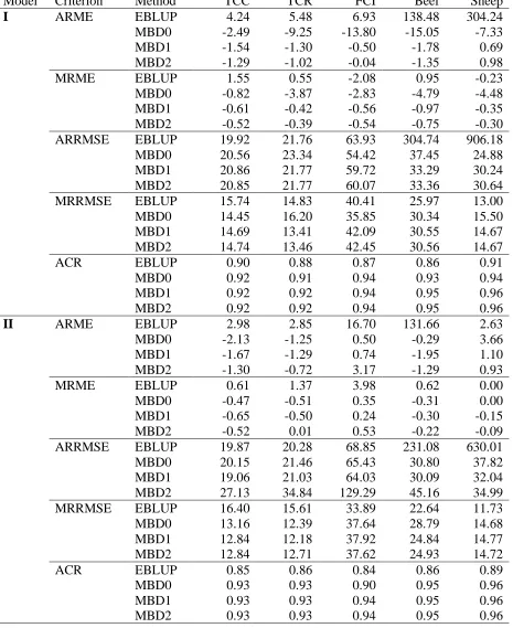
In the second stage of the simulation study, we compared the two variable specific estimators

EBLUP and MBD0 with the two multi-purpose estimators MBD1 and MBD2. Table 4

presents the average and median relative mean errors and relative RMSEs, as well as the

average coverage rates, generated by these four estimators for the five variables TCC, TCR,

FCI, Cattle and Sheep under the ‘reasonably specified’ Models I and II. These results show

that under the better fitting Model II, there is little, if any, difference in the average relative

mean errors of the multi-purpose estimators MBD1 and MBD2 compared with the average

substantially better than MBD0 and EBLUP. In terms of relative RMSE, the results are more

equivocal. Under Model I there is little to choose between MBD0, MBD1 and MBD2 in terms

of average relative RMSE, with the corresponding performance of EBLUP rather more

fragile. When one turns to the better fitting Model II, however, it is clear that the better

multipurpose approach is MBD1. By considering median, rather than average, values of

relative mean error and relative RMSE, we also see that the estimation performances of the

multipurpose estimators MBD1 and MBD2 appear to be more robust than those of the

variable specific estimators MBD0 and EBLUP. Finally, we note that the average coverage

rates of all three direct estimators are quite similar under both Models I and II and dominate

the corresponding average coverage performance of EBLUP. Overall it seems clear that for

our data set the multi-purpose estimator MBD1 is the estimator of choice for these five

variables.

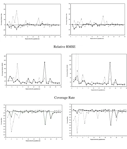
Figure 4 shows the region-specific relative mean errors, relative RMSEs and coverage rates

for TCC under Models I and II for EBLUP, MBD0, MBD1 and MBD2. The superior

efficiency of all estimators under Model II (after allowing for the outliers in regions 3 and 21)

is evident, as is the superior performance of MBD2. A similar pattern of results was observed

for TCR, FCI, Cattle and Sheep.

The unstable performance of EBLUP for the Cattle and Sheep variables in Table 4 is

noteworthy. Upon investigation we found that the anomalous results for Cattle were caused

by the presence of negative estimates for this variable in two regions (11 and 14), which were

themselves the result of zero values in the data. In particular, in region 11 there were 1283

zeros in the simulated population of 1586 values. This resulted in 185 negative estimates out

of the 1000 simulated for this region. Similarly in the region 14, there were 1972 zeros in the

2182 values in the simulated population, leading to 354 negative estimates. A similar reason

lay behind the EBLUP results for Sheep. In this case, however, in region 3 there were only 11

non-zero values for Sheep in a simulated population of size 189, leading to 223 negative

estimates, while in region 18 a majority of zero values for Sheep lead to 323 negative

estimates.

As noted earlier, our results indicate that multi-purpose estimation based on MBD1 is

preferable to that based on MBD2. Consequently, in Table 5 we contrast the performances of

for the three variables (Crops, Equity and Debt) that contain a large number of zeros. The

superior performance of MBD1 is obvious, as is the poor performance of EBLUP for these

variables. Note that these results are based on Model I, since Model II cannot be fitted to

these variables. In Table 6 we show that there is little change in the average performance of

MBD1 when the set of variables determining the multi-purpose weights used by this estimator

is extended from the original K = 5 variable set (TCC, TCR, FCI, Cattle, Sheep) to the entire

K = 8 variable set (TCC, TCR, FCI, Cattle, Sheep, Crops, Equity, Debt). Again, note that this

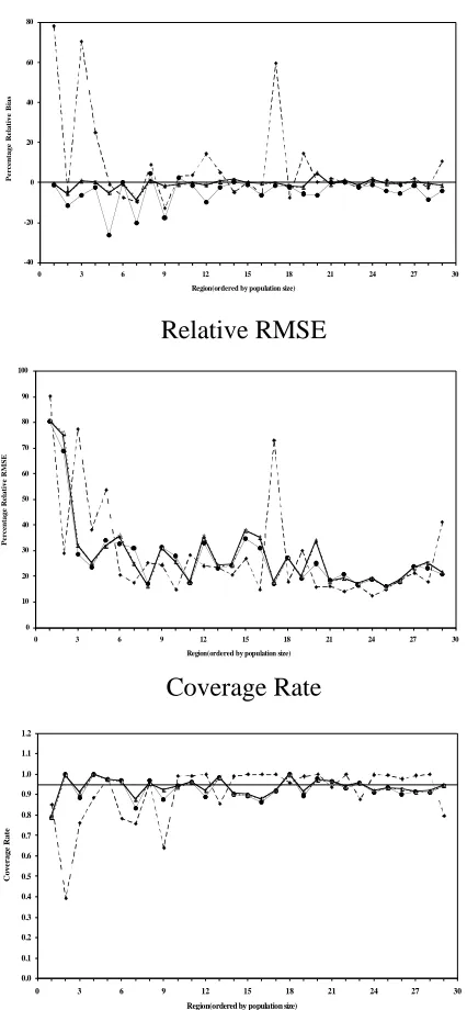
extension is only possible under Model I. Finally, in Figure 5 we show the overall

region-specific superior performance of MBD1 (under either K = 5 or K = 8) for the variable Debt.

Similar region-specific performances (not shown here) were observed for Crops and Equity.

6. Discussion and Further Research

The empirical results reported in the previous section are evidence that the MBD estimator

(14), particularly when combined with the multipurpose weights (19), can perform well and

represents a real alternative to the EBLUP, with the associated easy to calculate MSE

estimator (18) providing good coverage performance. Furthermore, they indicate that the

MBD approach may be more robust than EBLUP in the realistic situation where (10) is a

working model, rather than the (unknown) true model.

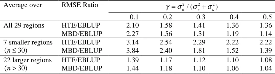
These results should not be taken as a blanket recommendation for MBD over EBLUP,

however. As noted in section 4, if one sets practical considerations aside, then EBLUP must

be the estimation method of choice when (9) actually holds. In such a case, the extent of the

efficiency gain over MBD will depend on both the distribution of the auxiliary variables as

well as the sample distribution across the small areas. To illustrate this, we return to the

Australian broadacre farm population used in the previous section, but this time carry out a

model-based simulation, first generating population values for TCC under the random

intercepts model (Model 1 in Table 2) with ! and !_e2 set at their fitted population values and

with different values of !_u2 chosen in order to obtain a range of values for the intra area

correlation ! ="_u2 / ("_e2+"_u2) , and then sampling from this simulated population using the

same regionally stratified design as used in the simulation study reported in the previous

section. Table 7 sets out the results of this simulation, in terms of the square root of the ratio

of the average empirical MSE of the Horvitz-Thompson estimator (HTE) of a regional total to

HTE/EBLUP), and the corresponding ratio (denoted MBD/EBLUP) of the average empirical

MSE of the MBD estimator of a regional total to that of the same EBLUP. Note that values of

these ratios for averages over all 29 regions as well as over regions with smaller sample sizes

and those with larger sample sizes are given. These clearly show that in the case where all

model assumptions are valid, the EBLUP, as one would expect, dominates both the MBD as

well as the conventional direct estimator (HTE). However, the extent of this dominance

decreases significantly as the strength of the regional effect increases, particular for regions

with larger sample sizes. The MBD in turn dominates the HTE except where the regional

effect is small, in which case we see that the EBLUP weights used in the MBD introduce

slightly more variance than they eliminate bias.

Before closing, we also mention a number of issues that impact on the utility of the MBD

estimator that remain unresolved. For example, negative weights, which occurred in some

regions in the simulation study reported in the previous section, can lead to impossible (i.e.

negative) estimates. Since such values are easily identified, they should not cause problems in

real life. However, the problem remains of how to modify the weights (13) to ensure they are

strictly positive. A related issue that has already been noted is the impact of outlier Y-values

on (14). Certainly this estimator, because it is a linear combination of just the small area data

values, is more susceptible to outliers in these values than the EBLUP estimator (11).

Methods for dealing with negative weights under ‘standard’ regression models have been

discussed in the literature (Huang and Fuller, 1978; Bardsley and Chambers, 1984; Deville

and Sarndal, 1992; Chambers, 1996) but their application in the context of mixed models

remains to be explored. Further, the data set used in section 5 involved skewed data as well as

a potential nonlinear relationship between the survey and auxiliary variables. It is possible to

adapt the MBD approach for small area estimation when variables are linear on a transformed

scale. The authors will report on this research in another paper.

References

Bardsley, P. and Chambers, R. L. (1984). Multipurpose estimation from unbalanced samples.

Applied Statistics33, 290 - 299.

Bates, D.M. and Pinheiro, J.C. (1998). Computational methods for multilevel models.

Available from http://franz.stat.wisc.edu/pub/NLME/

Chambers, R.L. (1996). Robust case-weighting for multipurpose establishment surveys.

Deville, J. C. and Särndal, C.-E. (1992). Calibration estimators in survey sampling. Journal of

the American Statistical Association87, 376 - 382.

Hidiroglou, M. A., Estavao, V. M. and Arcaro, C. (2000). Generalised estimation system and

future enhancements. In ICES-II Proceedings of the Second International Conference on

Establishment Surveys, pp 687-696. Alexandra, Virginia: American Statistical Association.

Huang, E. T. & Fuller, W. A. (1978). Nonnegative regression estimation for survey data.

Proceedings of the American Statistical Association, 300 – 305.

Prasad, N.G.N and Rao, J.N.K. (1990). The estimation of the mean squared error of

small-area estimators. Journal of the American Statistical Association 85, 163-171.

Rao, J. N. K. (2003). Small Area Estimation. New York: Wiley.

Royall, R.M. (1976). The linear least-squares prediction approach to two-stage sampling.

Journal of the American Statistical Association 71, 657-664.

Royall, R.M. and Cumberland, W.G. (1978). Variance Estimation in Finite Population

Table 1 Regional population and sample sizes

Region N n Region N n

1 79 6 16 2683 60

2 115 10 17 2689 60

3 189 30 18 2847 34

4 330 25 19 3056 74

5 388 36 20 3139 51

6 465 19 21 3910 73

7 604 36 22 4486 117

8 729 40 23 4550 80

9 737 30 24 4587 95

10 964 30 25 5368 83

11 1586 51 26 5528 103

12 1778 62 27 6489 108

13 1984 55 28 6980 81

14 2182 47 29 10933 77

15 2607 79

Table 2 Different mixed model specifications considered in the simulations

Model Model Type X Z

I Random Intercepts Intercept included Intercept only

II Random Slopes Intercept included Intercept + Size

III Random Slopes with

fixed intercept

Intercept included Size only

IV Random Slopes with

zero intercept

Intercept excluded Size only

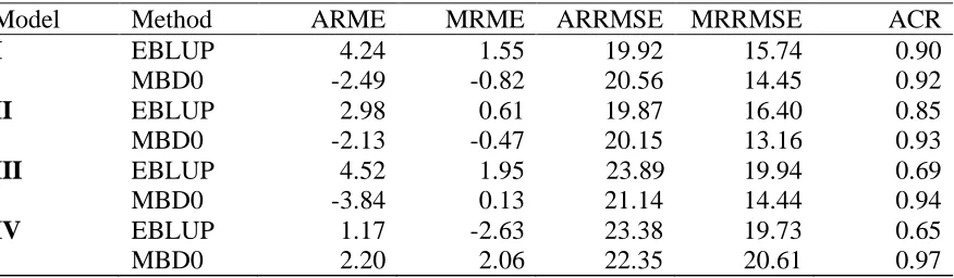
Table 3 Average (ARME) and median (MRME) values of relative mean error, average (ARRMSE) and median (MRRMSE) values of relative RMSE and average (ACR) coverage rates for TCC

Model Method ARME MRME ARRMSE MRRMSE ACR

EBLUP 4.24 1.55 19.92 15.74 0.90

I

MBD0 -2.49 -0.82 20.56 14.45 0.92

EBLUP 2.98 0.61 19.87 16.40 0.85

II

MBD0 -2.13 -0.47 20.15 13.16 0.93

EBLUP 4.52 1.95 23.89 19.94 0.69

III

MBD0 -3.84 0.13 21.14 14.44 0.94

IV EBLUP 1.17 -2.63 23.38 19.73 0.65

Table 4 Average and median relative mean error (ARME, MRME), average and median relative RMSE (ARRMSE, MRRMSE) and average coverage rate (ACR) for five variables best suited to linear mixed modelling

Model Criterion Method TCC TCR FCI Beef Sheep

I ARME EBLUP 4.24 5.48 6.93 138.48 304.24

MBD0 -2.49 -9.25 -13.80 -15.05 -7.33

MBD1 -1.54 -1.30 -0.50 -1.78 0.69

MBD2 -1.29 -1.02 -0.04 -1.35 0.98

MRME EBLUP 1.55 0.55 -2.08 0.95 -0.23

MBD0 -0.82 -3.87 -2.83 -4.79 -4.48

MBD1 -0.61 -0.42 -0.56 -0.97 -0.35

MBD2 -0.52 -0.39 -0.54 -0.75 -0.30

ARRMSE EBLUP 19.92 21.76 63.93 304.74 906.18

MBD0 20.56 23.34 54.42 37.45 24.88

MBD1 20.86 21.77 59.72 33.29 30.24

MBD2 20.85 21.77 60.07 33.36 30.64

MRRMSE EBLUP 15.74 14.83 40.41 25.97 13.00

MBD0 14.45 16.20 35.85 30.34 15.50

MBD1 14.69 13.41 42.09 30.55 14.67

MBD2 14.74 13.46 42.45 30.56 14.67

ACR EBLUP 0.90 0.88 0.87 0.86 0.91

MBD0 0.92 0.91 0.94 0.93 0.94

MBD1 0.92 0.92 0.94 0.95 0.96

MBD2 0.92 0.92 0.94 0.95 0.96

II ARME EBLUP 2.98 2.85 16.70 131.66 2.63

MBD0 -2.13 -1.25 0.50 -0.29 3.66

MBD1 -1.67 -1.29 0.74 -1.95 1.10

MBD2 -1.30 -0.72 3.17 -1.29 0.93

MRME EBLUP 0.61 1.37 3.98 0.62 0.00

MBD0 -0.47 -0.51 0.35 -0.31 0.00

MBD1 -0.65 -0.50 0.24 -0.30 -0.15

MBD2 -0.52 0.01 0.53 -0.22 -0.09

ARRMSE EBLUP 19.87 20.28 68.85 231.08 630.01

MBD0 20.15 21.46 65.43 30.80 37.82

MBD1 19.06 21.03 64.03 30.09 32.04

MBD2 27.13 34.84 129.29 45.16 34.99

MRRMSE EBLUP 16.40 15.61 33.89 22.64 11.73

MBD0 13.16 12.39 37.64 28.79 14.68

MBD1 12.84 12.18 37.92 24.84 14.77

MBD2 12.84 12.71 37.62 24.93 14.72

ACR EBLUP 0.85 0.86 0.84 0.86 0.89

MBD0 0.93 0.93 0.90 0.95 0.96

MBD1 0.93 0.93 0.94 0.95 0.96

Table 5 Average relative mean error (ARME), average relative RMSE (ARRMSE) and average coverage rate (ACR) for EBLUP, MBD0 and MBD1 for variables with many zeros. Model I is assumed.

Variable ARME ARRMSE ACR

EBLUP MBD0 MBD1 EBLUP MBD0 MBD1 EBLUP MBD0 MBD1

Crops 90.31 0.003 -0.21 123.96 23.53 22.92 0.95 0.96 0.96

Equity 4.36 -9.32 -1.20 18.51 19.14 17.05 0.88 0.92 0.94

Debt 8.39 -4.94 -0.96 29.02 27.71 28.57 0.91 0.93 0.93

Table 6 Average relative mean error (ARME), average relative RMSE (ARRMSE) and

average coverage rate (ACR) for multi-purpose weighting (MBD1) based on original K = 5

and extended K = 8 variable sets. Model I is assumed.

Variable K = 5 K = 8

ARME ARRMSE ACR ARME ARRMSE ACR

TCC -1.54 20.86 0.92 -1.08 20.91 0.92

TCR -1.30 21.77 0.92 -0.80 21.83 0.92

FCI -0.50 59.72 0.94 0.21 60.22 0.94

Cattle -1.78 33.29 0.95 -1.05 33.49 0.95

Sheep 0.69 30.24 0.96 1.24 31.06 0.96

Crops -0.21 22.92 0.96 -0.20 22.97 0.96

Equity -1.20 17.05 0.94 -0.72 17.14 0.94

Debt -0.96 28.57 0.93 -0.68 28.74 0.93

Table 7 Ratio of the square root of the average mean squared errors of Horvitz-Thompson (HTE) and MBD estimates of regional totals to EBLUP-based estimates of the same totals. Sample design is stratified by region, with SRSWOR within regions and sample allocations as in Table 1. The data were generated using Model 1 of Table 4, and this model was also assumed by both the EBLUP and MBD methods.

! ="u 2

/ ("_e2 +"_u2)

Average over RMSE Ratio

0.1 0.2 0.3 0.4 0.5

HTE/EBLUP 2.10 1.58 1.41 1.36 1.36

All 29 regions

MBD/EBLUP 2.27 1.56 1.31 1.19 1.14

HTE/EBLUP 3.14 2.54 2.29 2.22 2.22

7 smaller regions

(n!30) MBD/EBLUP 3.84 2.40 1.81 1.52 1.39

HTE/EBLUP 1.39 1.17 1.12 1.10 1.08

22 larger regions

Figure 1 Regional relative mean errors for EBLUP (dashed line) and MBD0 (solid line) for TCC under models I (top left), II (top right), III (bottom left) and IV (bottom right).

-40 -20 0 20 40 60 80

0 3 6 9 12 15 18 21 24 27 30 Region(ordered by population size)

P e r c e n ta g e R e la ti v e B ia s -40 -20 0 20 40 60 80

0 3 6 9 12 15 18 21 24 27 30 Region(ordered by population size)

P e r c e n ta g e R e la ti v e B ia s -40 -20 0 20 40 60 80

0 3 6 9 12 15 18 21 24 27 30 Region(ordered by population size)

P e r c e n ta g e R e la ti v e B ia s -40 -20 0 20 40 60 80

0 3 6 9 12 15 18 21 24 27 30 Region(ordered by population size)

P e r c e n ta g e R e la ti v e B ia s

Figure 2 Regional relative RMSEs for EBLUP (dashed line) and MBD0 (solid line) for TCC under models I (top left), II (top right), III (bottom left) and IV (bottom right).

0 20 40 60 80 100 120 140

0 3 6 9 12 15 18 21 24 27 30 Region(ordered by population size)

P e r c e n ta g e R e la ti v e R M S E 0 20 40 60 80 100 120 140

0 3 6 9 12 15 18 21 24 27 30 Region(ordered by population size)

P e r c e n ta g e R e la ti v e R M S E 0 20 40 60 80 100 120 140

0 3 6 9 12 15 18 21 24 27 30 Region(ordered by population size)

P e r c e n ta g e R e la ti v e M S E 0 20 40 60 80 100 120 140

0 3 6 9 12 15 18 21 24 27 30 Region(ordered by population size)

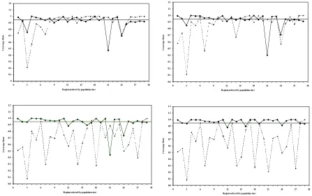
Figure 3 Regional coverage rates for EBLUP (dashed line) and MBD0 (solid line) for TCC under models I (top left), II (top right), III (bottom left) and IV (bottom right).

0 0.1 0.2 0.3 0.4 0.5 0.6 0.7 0.8 0.9 1 1.1 1.2

0 3 6 9 12 15 18 21 24 27 30 Region(ordered by population size)

C o v e r a g e R a te 0.0 0.1 0.2 0.3 0.4 0.5 0.6 0.7 0.8 0.9 1.0 1.1 1.2

0 3 6 9 12 15 18 21 24 27 30 Region(ordered by population size)

C o v e r a g e R a te 0.0 0.1 0.2 0.3 0.4 0.5 0.6 0.7 0.8 0.9 1.0 1.1 1.2

0 3 6 9 12 15 18 21 24 27 30 Region(ordered by population size)

C o v e r a g e R a te 0.0 0.1 0.2 0.3 0.4 0.5 0.6 0.7 0.8 0.9 1.0 1.1 1.2

0 3 6 9 12 15 18 21 24 27 30 Region(ordered by population size)

Figure 4 Regional performances of EBLUP (dashed line), MBD0 (thin line), MBD1 (thick line) and MBD2 (dotted line) for TCC under models I (left) and II (right).

Relative Mean Error

-40 -20 0 20 40 60 80

0 3 6 9 12 15 18 21 24 27 30 Region(ordered by population size)

P e r c e n ta g e R e la ti v e B ia s -40 -20 0 20 40 60 80

0 3 6 9 12 15 18 21 24 27 30 Region(ordered by population size)

P e r c e n ta g e R e la ti v e B ia s Relative RMSE 0 20 40 60 80 100 120 140

0 3 6 9 12 15 18 21 24 27 30 Region(ordered by population size)

P e r c e n ta g e R e la ti v e R M S E 0 20 40 60 80 100 120 140

0 3 6 9 12 15 18 21 24 27 30 Region(ordered by population size)

P e r c e n ta g e R e la ti v e R M S E Coverage Rate 0 0.1 0.2 0.3 0.4 0.5 0.6 0.7 0.8 0.9 1 1.1 1.2

0 3 6 9 12 15 18 21 24 27 30 Region(ordered by population size)

C o v e r a g e R a te 0.0 0.1 0.2 0.3 0.4 0.5 0.6 0.7 0.8 0.9 1.0 1.1 1.2

0 3 6 9 12 15 18 21 24 27 30 Region(ordered by population size)

Figure 5 Regional performances of EBLUP (dashed line), MBD0 (thin line), MBD1 under K

= 5 (thick line) and MBD1 under K = 8 (dotted line) for Debt under model I.

Relative Mean Error

-40 -20 0 20 40 60 80

0 3 6 9 12 15 18 21 24 27 30 Region(ordered by population size)

P e r c e n ta g e R e la ti v e B ia s Relative RMSE 0 10 20 30 40 50 60 70 80 90 100

0 3 6 9 12 15 18 21 24 27 30 Region(ordered by population size)

P e r c e n ta g e R e la ti v e R M S E Coverage Rate 0.0 0.1 0.2 0.3 0.4 0.5 0.6 0.7 0.8 0.9 1.0 1.1 1.2

0 3 6 9 12 15 18 21 24 27 30 Region(ordered by population size)