Robustness in the graph topology of a common adaptive controller

ADAPTIVE CONTROLLER

MARK FRENCH†_{, ACHIM ILCHMANN}‡_{, ANDEUGENE P. RYAN}§

Abstract. For anym-input,m-output, finite-dimensional, linear, minimum-phase plantP with first Markov parameter having spectrum in the open right-half complex plane, it is well known that the adaptive output feedback controlC, given byu=−ky, k˙ =kyk2_{, yields a closed-loop system}

[P, C] for which the state converges to zero, the signalkconverges to a finite limit, and all other sig-nals are of classL2_{. It is first shown that these properties continue to hold in the presence ofL}2_-input

andL2_{-output disturbances. By establishing gain function stability of an appropriate closed-loop}

operator, it is proved that these properties also persist when the plantP is replaced by a stabilizable and detectable linear plantP1 within a sufficiently small neighbourhood ofP in the graph topology,

provided that the plant initial data and theL2_{magnitude of the disturbances are sufficiently small.}

Example 9 of Georgiou & Smith (IEEE Trans. Autom. Control42(9) 1200–1221, 1997) is revisited. Unstable behaviour for large initial conditions and/or largeL2_{disturbances is shown, demonstrating}

that the bounds obtained from theL2 _{theory are qualitatively tight: this contrasts with theL}∞

-robustness analysis of Georgiou & Smith which is insufficiently tight to predict the stable behaviour for small initial conditions and zero disturbances.

Keywords: adaptive control, gap metric, robust stability.

1. Introduction. In an important paper in 1997, the well-established concept of the gap metric for linear systems [9] was extended to a nonlinear setting by Georgiou and Smith [3]. The central property analysed in the nonlinear gap framework is that of robust stability, i.e. the property that, if _W is some requisite class (for example,

L∞_orL2_{) to which the signals of a nominal closed-loop plant/controller configuration}

belong, then the closed-loop signals remain inW if the nominal plant is replaced by another plant which is sufficiently close in the gap sense. Gain function stability (a concept made precise in Sub-section 2.3) of the closed-loop operator mapping external disturbances to the input and output of the nominal plant provides a sufficient con-dition for robust stability (however, in contrast with the results in the linear setting, gain function stability is not a necessary condition for robust stability in the nonlinear setting). The nonlinear gap framework has been used to investigate the robustness (or lack of robustness) of certain classical adaptive controllers and variants thereof.

1. Working in anL∞ _{setting, Example 9 of [3] (see also [4]) considers the controller}

(ubiquitous in the adaptive control literature)

u=−ky, k˙ =y2 (1.1)

applied to the scalar linear plant ˙y = ay+u, for some a ∈ R_{, and shows that}

the closed-loop operator mapping external disturbances onto the input and output of the nominal plant is not gain function stable. Whilst the lack of gain function stability does not preclude robust stability, numerical and other informal evidence was presented which suggested that, with non-zero initial conditions, the closed-loop

∗_{This research was supported by Deutsche Forschungsgemeinschaft, grant IL 25/3-1}

†_{School of Electronics and Computer Science, University of Southampton, Southampton SO17}

1BJ, UK, [email protected]

‡_{Institut f¨ur Mathematik, Technische Universit¨at Ilmenau, Weimarer Straße 25, 98693 Ilmenau,}

DE, [email protected]

§_{Department of Mathematical Sciences, University of Bath, Claverton Down, Bath BA2 7AY,}

UK,[email protected]

system is not robustly stable, even in the absence of disturbances. One consequence of the results of the present paper is to clarify the latter suggestion: we prove that, in the absence of disturbances, the closed-loop system is – with sufficiently small initial data – robustly stable but fails to be robustly stable for large initial data.

2. In [1], the nonlinear gap framework is used in an L2 _{setting to establish robust}

stability properties of the controller u= −k14y, ˙k = y2 when applied to (a) single-input, single-output, linear, minimum-phase, relative-degree-one, nominal plants with positive high-frequency gain, and (b) a class of perturbed plants, where the gap metric distance between the nominal and perturbed plants is constrained by a function of the norms of the external disturbances.

The present paper shows that the analysis developed in [1] can also be applied to the more familiar adaptive controller (1.1) (and its multivariable counterpart). This is considered to be important as such controllers form the basis for many adaptive designs see e.g. [5, 6]. In particular, in anL2 _{setting, we establish a robust stability}

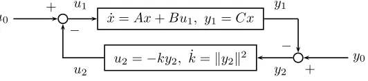
result for nominalm-input,m-output, finite-dimensional, stabilizable and detectable linear plants (A, B, C) which are minimum phase and are such that the first Markov parameter CB has its spectrum in the open right-half complex plane (we denote the class of such plants by _M). With reference to Figure 1.1, in the absence of external disturbances (that is, with u0 = 0 = y0), it is well known that, for every plant in_M and all initial plant/controller data (x0_{, k}0₎

∈ Rn_×R_{+ (}R_{+ := [0,∞)),}

the closed loop is such that (i) u1, y1 ∈ L2_(R+,Rm_{), (ii) x(t) → 0 as t → ∞, and} (iii) k(t) → k∞ _{∈ R}

+ as t → ∞. First, we show that properties (i)-(iii) persist

u0 u1 x˙ =Ax+Bu1, y1=Cx y1

u2=₋ky2, k˙ =_ky2_k2 _y0

u2 y2

−

+ +

−

Fig. 1.1_. The adaptive closed-loop system.

under external disturbancesu0, y0_∈L2_(R+,Rm_{). Secondly, we consider the question} of robust stability of the closed-loop with respect to both external L2 _disturbances

and perturbations of the plant (A, B, C): to what extent do the above properties (i)–(iii) persist if (A, B, C)_{∈ M}is perturbed to another m-input, m-output, linear, finite-dimensional, stabilizable and detectable plant (Ap, Bp, Cp)6∈ M?

An appropriate conceptual framework in which to pose and answer such questions is provided by the gap metric. We show that properties (i)-(iii) persist if (A, B, C) and (Ap, Bp, Cp) are sufficiently close in the gap metric. The associated bounds on the robust stability margin have a semi-global nature insofar as they depend on the “size” of the external disturbances and initial data.

RH∞_{, the class of rational functions that are analytic and bounded on the open half}

planeC_+:={λ∈C_{|Re(λ)>0}. In particular, there existNi, Di∈RH}∞_{such that}

ˆ

Pi=NiDi−1, Ni∗Ni+Di∗Di= 1, i= 1,2. (1.2) For (i, j) = (1,2),(2,1), define the directed gap

~δ0( ˆPi,Pˆj) := inf

©

k(∆N,∆D)_kH∞

¯

¯ ∆N,∆D_∈RH∞, Pˆj= (Ni+ ∆N)(Di+ ∆D)−1

ª

,

(with the convention inf _∅:= +_∞). The linear gap between ˆP1and ˆP2 is given by

δ0( ˆP1,P2ˆ )_≡δ0( ˆP2,P1ˆ) = max©~δ0( ˆP1,P2ˆ ), ~δ0( ˆP2,P1ˆ)ª. (1.3)

We remark that the gap between the following plants ˆP1and ˆP2tends to zero asε→0:

ˆ

P1(s) P2ˆ (s) Reference

i) 1

s₋θ

|λ|2

(s−λ)(s−λ¯)(s−θ), Re(λ)≤ −ε

−1 _[1]

ii) 1

s₋θ

N(M−s)

(N+s)(M+s)(s₋θ), N, M ≥ε

−1 _{§3.4, Example 3.10}

iii) 1

s₋θ

(M₋s)

(M+s)(s₋θ), M ≥ε

−1

§4.5, see also [3]

Example i) is the classical Rohrs’ example [7] which first drew the attention of the adaptive control community to the robustness issue. As observed in [1], Example ii) is of particular interest since ˆP2exhibits none of the classical assumptions of adaptive control: in particular, the sign of the high frequency gain and the relative degree of

ˆ

P2differ from those of the nominal plant ˆP1and, moreover, ˆP2is not minimum phase. Example ii) is considered in more detail in Section 3.4. Example iii) is comprised of an all-pass factor in series with the nominal plant and is considered extensively in Section 4. Example iii) also coincides with Example 9 in [3] to which our generalL2

theory applies to conclude robust stability provided the initial data andL2_disturbance

norms are sufficiently small. In Section 4, we additionally prove the lack of robustness when the initial data or theL2 _{disturbances are large. Moreover, we clarify some of}

the informal arguments in theL∞ _{setting of [3].}

2. Background concepts and terminology. The material in this section is based on [3, Section II] and [1, Section 2].

2.1. Preliminaries. Whilst our goal is to establish stability of various config-urations of plant and controller, the nonlinear nature of the controller is such that finite-time blow up of solutions of the closed-loop system cannot be ruled outa priori. To accommodate the potential for such a behaviour in the analysis, we introduce the following artifacts. Let_X be a nonempty set and, for 0< ω _{≤ ∞}, let_Sω denote the set of locally integrable maps [0, ω) _{→ X}. For simplicity, we write _S := _S∞. For

0< τ < ω_{≤ ∞},Tτ :Sω→ S denotes the operator given by

Tτv :=

½

v(t), t_∈[0, τ) 0, otherwise.

With _{V ⊂ S} we associate spaces as follows: _Ve =

©

v_{∈ S}¯¯Tτv∈ V ∀τ >0

ª

, the extended space; _Vω =

©

v_{∈ S}ω

¯

¯Tτv∈ V ∀τ∈(0, ω)

ª

the ambient space. If v, w _{∈ V}a with v|I = w|I onI = dom(v)∩dom(w), then we writev=w. Note that_{V ⊂ V}e⊂ Va are strict inclusions and V∞=Ve.

For (f, g) _{∈ V}a × Va, the domains of f and g may be different; we adopt the convention dom(f, g) := dom(f)_∩ dom(g).

We define _{V ⊂ S} to be a signal space if, and only if, it is a vector space. In our applications, frequently_V will be a normed signal space, such asLp_(R+,Rm_{) for} 1 _≤p_{≤ ∞}, in which case,_Ve=Lploc(R+,Rm), Vω=Lploc([0, ω),Rm) forω ∈(0,∞]

and_Va =∪0<ω≤∞Lploc([0, ω),Rm). It is important to note thatVω6=Lp([0, ω),Rm). Throughout the paper we consider only those normed signal space _V which have the property that supτ≥0kTτxk <∞ implies x ∈ V. We observe that Lp(R+,Rm) for 1≤p≤ ∞is such a normed signal space . We will often writekxkτ=kTτxk.

For a normed signal space U and a Euclidean space Rn_{, we will also consider} subsets of spaces of the formV =Rn_{× U, which, on identifying eachθ∈R}n _{with the} constant signal t7→θ, can be thought of as a normed signal space with norm given byk(θ, x)k=p|θ|2_+kxk2

U.

2.2. Well posedness. A mappingQ:_X1→ X2 between signal spaces is said to

be causal if, and only if, for allτ >0,x, y ∈ X1,Tτx=Tτy impliesTτQx=TτQy. LetU andY be normed signal spaces and letP:Ua→ Ya andC:Ya→ Ua be causal mappings representing the plant and controller, respectively. Our central concern is the system of equations

[P, C] : y1=P u1, u2=Cy2, u0=u1+u2, y0=y1+y2 (2.1)

corresponding to the closed-loop feedback configuration as depicted in Figure 2.1.

u0 u1

y1 P

C y0

u2 y2

−

+ +

−

Fig. 2.1_.The closed-loop system[P, C].

By a solution of (2.1) we mean the following. For w0 = (u0, y0)_{∈ W} :=_{U × Y}, a pair (w1, w2) =¡(u1, y1),(u2, y2)¢_{∈ W}a× Wa,Wa :=Ua× Ya,is asolution of (2.1) if, and only if, (2.1) holds on dom(w1, w2). The (possibly empty) set of all solutions is denoted by_Xw0 :=

©

(w1, w2)_{∈ W}a× Wa|(w1, w2) solves (2.1)

ª

. The closed-loop system [P, C], given by (2.1), is said have: (a) the existence property if, and only if,

Xw0 6=∅; (b) theuniqueness property if, and only if, for eachw0∈ W,

( ˆw1,w2ˆ ),( ˜w1,w2˜ )∈ Xw0

=_⇒( ˆw1,w2ˆ ) = ( ˜w1,w2˜ ) on dom( ˆw1,w2ˆ )_∩dom ( ˜w1,w2˜ ).

Assume that [P, C] has the existence and uniqueness properties. For eachw0 _{∈ W}, define ωw0, 0 < ωw0 ≤ ∞, by the property [0, ωw0) := ∪( ˆw1,w2ˆ )∈Xw0dom( ˆw1,w2ˆ ) and define (w1, w2) ∈ Wa × Wa, with dom(w1, w2) = [0, ωw0), by the property (w1, w2)|[0,t) ∈ Xw0 for all t ∈ [0, ωw0). This construction induces an operator

HP,C :W → Wa× Wa, w07→(w1, w2).

The closed-loop system [P, C], given by (2.1), is said to be:

the operatorHP,C: W → Wa× Wa, w07→(w1, w2), is causal;

•globally well posed if, and only if, it is locally well posed and imHP,C⊂ We× We;

• W-stable if, and only if, it is locally well posed and imHP,C⊂ W × W;

•regularly well posed if, and only if, it is locally well posed and

∀w0_{∈ W} £ωw0 <∞ =⇒ Tωw0HP,C(w0)∈ W × W/

¤

. (2.2)

If [P, C] is globally well posed, then for eachw0∈ Wthe solutionHP,C(w0) exists on the half lineR_{+. Regular well posedness means that if the closed-loop system has}

a finite escape time ω > 0 for some disturbance (u0, y0) _{∈ W}, then at least one of the componentsu1, u2 ory1,y2 is not a restriction to [0, ω) of a function in_U or _Y, respectively. If [P, C] is regularly well posed and satisfies

∀w0∈ W £ ωw0<∞ =⇒ Tωw0HP,C(w0)∈ W × W

¤

,

there does not exist a solution of [P, C] with a finite escape time, and therefore [P, C] is globally well posed. However, global well posedness does not guarantee that each solution belongs toW × W; the latter is ensured by W-stability of [P, C]. Note also that neither regular nor global well posedness implies the other.

Our main concern will be the situation wherein the closed-loop system [P, C] is generated by a system of (nonlinear) differential equations. In this context, a globally well-posed system is a system with the property of existence and uniqueness of solutions and for which finite-time blow up does not occur: all (forward) solutions have maximal interval of existence [0,_∞). Regular well posedness usually follows from standard existence theory for differential equations when_W =L∞

×L∞_{. However,}

when _{W 6}=L∞

×L∞ _{(in this paper we are primarily interested in}

W = L2 ×L2_),

stronger properties of the underlying differential equations are required. As shall be shown, all closed-loop systems considered in this paper are regularly well posed.

2.3. Graphs and gain-function stability. In our investigation of robustness of stability properties of a closed-loop system, the concept of graphs and gain-function stability will play a central rˆole. Corresponding to a plant operatorP(respectively, the controller operatorC) is a subset of_W, called thegraph of the plant_GP (respectively, the controller_GC), defined as

GP =

½ µ

u P u

¶ ¯¯_¯

¯ u∈ U, P u∈ Y ¾

⊂ W, GC=

½ µ

Cy y

¶ ¯¯_¯

¯ Cy∈ U, y∈ Y ¾

⊂ W.

Note that in generalGP,GC6=W.

A causal operatorF:_{X → V}a whereX,V are subsets of normed signal spaces, is said to begain-function stable(orgf-stable) if, and only if, imF ⊂ Vand the following nonlinear so-calledgain-function is well defined:

g[F] : (r0,_∞)_→R_+,

r_7→g[F](r) = sup©_kTτF xk

¯

¯x_{∈ X} , _kTτxk ∈(r0, r], τ >0

ª

, (2.3)

where r0 := infx∈Xkxk < ∞. Observe that kF xkτ ≤ g[F](kxkτ). A closed-loop system [P, C] is said to be gf-stable if, and only if, it is globally well posed and

HP,C: W → We× Weis gf-stable.

Note the following facts: (i) global well posedness of [P, C] implies that imHP,C ⊂

[P, C] is _W-stable, then HP,C : W → GP × GC is a bijective operator with inverse

H_P,C−1 : (w1, w2) _7→ w1 +w2. To see (iii), note that imHP,C ⊂ W × W implies that imHP,C ⊂ GP × GC, and since for any w1 ∈ GP ⊂ W, w2 ∈ GC ⊂ W we have w1+w2 _{∈ W}, it follows that imHP,C ⊃ GP × GC. Therefore, we can think of an gf-stable HP,C as a surjective operator HP,C: W → GP × GC. The inverse of

HP,C :W → GP× GC is obviouslyHP,C−1 : (w1, w2)7→w1+w2.

Finally, with a closed-loop system [P, C], we associate the following two parallel projection operators: ΠP//C :W → Wa, w07→w1, and ΠC//P :W → Wa,w07→w2. Clearly,HP,C =

¡

ΠP//C,ΠC//P¢and ΠP//C+ ΠC//P =I. Therefore, gf-stability of one of the operators ΠP//C and ΠC//P implies the gf-stability of the other, and so gf-stability of either operator implies gf-stability of the closed-loop system [P, C].

2.4. The nonlinear gap. The essence of the paper is an investigation (in a spe-cific adaptive control context) of the persistence, or otherwise, of stability properties of a globally well-posed closed-loop system [P, C] under “sufficiently small” pertur-bations of the plant or, in other words, when the plant P is replaced by any plant sufficiently “close” toP. Here, plantsP1andP2are deemed close if, and only if, their respective graphs are close in the gap sense of [3], outlined next.

Let Γ := ©P : _Ua → Ya

¯

¯ P is causalª and, for P1, P2 _∈ Γ, define the (possibly empty) setOP1,P2 := ©Φ :GP1→ GP2

¯

¯Φ is causal, bijective, and Φ(0) = 0ª. Write

~δ(P1, P2) := inf

Φ∈OP1,P2

sup x∈GP1\{0}, τ >0

µ_k(Φ−I)|

GP1xkτ

kx_kτ

¶

,

with the convention that~δ(P1, P2) :=_∞if_OP1,P2 =∅. The nonlinear gapδis

δ: Γ_×Γ_→[0,_∞], (P1, P2)_7→δ(P1, P2) := max_{~δ(P1, P2), ~δ(P2, P1)_}. (2.4)

which provides a generalisation of the standard definition of the linear gapδ0 (previ-ously discussed briefly in the Introduction). To explain this, some notation is needed. Forq, m∈N_{, letRq,mdenote the set of proper, rational, (q×m)-matrix-valued}

func-tions and let H∞

q,m denote the set of analytic and bounded Cq×m-valued functions on the open right half plane C_{+ := {λ ∈} C_{| Re(λ) > 0}. By RH}∞

q,m, we denote the class of functions inRq,m that are analytic in C+. It is known, see for example

[8, pp. 74-75, 261-262], that any P ∈ Rq,m has a normalised right co-prime factor-ization, that is, P = N D−1_{, where N}

∈ RH∞

q,m, D ∈ RHm,m∞ , D has an inverse in Rm,m, and N∗_{N +D}∗_{D =Im, where N}∗_{(s) := N(}

−s¯)T. Let _U =L2_(R+,Rm_),

Y=L2_(R+,Rq_{) for somem, q}

∈N_{and associate, with ˆP ∈Rq,m, the linear operator}

P: _Ue → Ye, u 7→y :=L−1( ˆP)? u, where L denotes the Laplace transform and ? denotes convolution. We refer toP as a linear plant with associated transfer function

ˆ

P _∈ Rq,m. For i = 1,2, let Pi: Ue → Ye be linear plants with associated strictly proper rational transfer functions ˆPi =NiD−1i , where (Ni, Di) ∈ RHq,m∞ ×RHm,m∞ are right co-prime factors (analogous to (1.2)), and let Πi : _Ue× Ye → GPi denote

the orthogonal projection onto the closed subspaceGPi, respectively. The linear gap

between these plants is defined as in (1.3), with

~δ0( ˆPi,Pˆj) := inf

©

k(∆N,∆D)_kH∞

¯

¯ ∆N _∈RHq,m∞ , ∆D∈RHm,m∞ , ˆ

Pj = (Ni+ ∆N)(Di+ ∆D)−1

ª

In [3, Proposition 5] it is shown that if max_{k(Π2−Π1) Π1k,k(Π1−Π2) Π2k}<1, then ~δ(P1, P2) = _k(Π2−Π1) Π1k, and in [2, Lemma 2] it is shown thatk(Π2−Π1) Π1k = ~δ0( ˆP1,P2ˆ ) if~δ0( ˆP1,P2ˆ )<1, the conjunction of which yields

~δ(P1, P2) = ~δ0( ˆP1,P2ˆ ), if δ0( ˆP1,P2ˆ )<1. (2.5)

The topology induced onRq,m by the gapδ0 is called the graph topology [8, p. 235]; note that the graph topology on Γ induces the graph topology onRq,mvia the subset topology and the Laplace transformL.

3. System classes and the adaptive controller. We are interested in the control of linearm-inputm-output stabilisablen-dimensional state space realisations of transfer functions inRm,m, i.e. systems of the form

˙

x(t) =A x(t) +B u1(t), x(0)_∈Rn_{, y1(t) =Cx(t). (3.1)}

Henceforth, we fix (arbitrarily) the number m _≥ 1 of inputs/outputs but allow for variation of the state space dimensionn. We denote this system class by

Pn = {(A, B, C)∈En | n≥m, (A, B, C) is stabilizable and detectable} (3.2)

whereEn :=Rn×n×Rn×m×Rm×n. We also define the subclass of minimum-phase systems with “high-frequency gain”CB having spectrum inC_+,

f

Mn =

½

(A, B, C)_{∈ P}n

¯ ¯ ¯

¯ σ(CB)⊂C+, det ·

sIn−A B

C 0

¸

6

= 0_∀s_∈C₊ ¾

. (3.3)

Observe that, for each (A, B, C)∈Mfn, there exists an element of its similarity orbit

{(T AT−1_{, T B, CT}−1₎

|T _∈Rn×n _{invertible} such that}

T AT−1=

·

A1 A2 A3 A4

¸

, T B=

·

0

B2

¸

=

·

0

CB

¸

, CT−1=£0 I¤

where σ(B2) ⊂C_{+ and, by the minimum-phase property, A1 has spectrum in the}

open left half complex planeC_{−. Therefore, we introduce}

Mn :=

 

(A, B, C)∈ Pn ¯ ¯ ¯ ¯ ¯ ¯

A=

·

A1 A2 A3 A4

¸

, B=

·

0

B2

¸

, C= [0 I],

B2, A4∈Rm×m_{, σ(A1)⊂}C_{−, σ(B2)⊂}C₊  

. (3.4)

For a system of class_Mn, (3.1) may be expressed in the equivalent form

˙

z(t) =A1z(t) +A2y1(t), z(0) =z0_∈Rn−m ˙

y1(t) =A3z(t) +A4y1(t) +B2u1(t), y1(0) =y0 1 ∈Rm

¾

, (z0, y01) =x0. (3.5)

We will have occasion to identify _Pn with a subspace of Euclidean space Rn 2_+2mn by identifying a plant θ = (A, B, C) with a vector θ consisting of the elements of the plant matrices, ordered lexigraphically. With normed signal spacesU and Y and (θ, x0_{)∈ P}

n×Rn, we associate the causal plant operator

e

P(θ, x0) : _Ua → Ya, u17→Pe(θ, x0)(u1) :=y1, (3.6)

of maps _Ua → Ya. Furthermore, for (θ, x0) = (A, B, C, x0) ∈ Pn ×Rn, Pe(θ, x0) corresponds to a stabilizable and detectable realisation ofC(sIn−A)−1B ∈Rm,m.

Our objective is to study, in the context of systems of form (3.1), the common adaptive strategy

u2(t) =₋k(t)y2(t), k˙(t) =_ky2(t)_k2, k(0) =k0_∈R_{+, (3.7)}

with the associated control operator, parameterized byk0_{, denoted by}

e

C(k0) :Ya→ Ua, y27→Ce(k0)(y2) :=u2. (3.8)

Note thatCe is a map fromR_{+ to the space of causal mapsYa→ Ua.}

In particular and with reference to Figure 2.1, we will study properties of the closed-loop system [Pe(θ, x0_),Ce(k0_{)], generated by the application of the adaptive}

controller (3.8) to system (3.1), in the presence of disturbances (u0, y0)_{∈ W}satisfying the interconnection equations

u0 = u1+u2, y0 = y1+y2. (3.9)

Results will be given for systems (3.5) of class (3.4) (such systems will later play the rˆole of the nominal plant) and for the more general class of systems (3.1), (3.2) (such systems which will later play the rˆole of the perturbed plant).

3.1. Properties of the interconnection of the adaptive controller with the general linear plant. In this section we investigate the interconnection of the adaptive controller (3.7) (with associated operator Ce(k0_{)) and any plant in the form}

(3.1) (with associated operatorPe(θ, x0_{)), where (θ, x}0_{, k}0_{)∈ P}

n×Rn×R+.

Proposition 3.1. _{Let n ≥ m, (θ, x}0_{, k}0_{) ∈ P}

n ×Rn ×R+ and u0, y0 ∈ L∞

loc(R+,Rm). Then the closed-loop initial-value problem given by (3.1),(3.7),(3.9)

has the following properties: (i) there exists a unique maximal solution(x, k) : [0, ω)→

Rn _×R_{+, 0 < ω ≤ ∞; (ii) if k ∈ L}∞_{([0, ω),}R_{+), then ω = ∞; (iii) if y2 ∈}

L2_{([0, ω),R}m_{), thenω=}

∞.

Proof. (i) follows from the theory of ordinary differential equations. (ii): If k_∈L∞_{([0, ω),R}

+), then consider the following subsystem of the initial-value

problem (3.1), (3.7): ˙x(t) = Ax(t) +B£u0(t) +k(t)y2(t)¤. Integration, together with elementary estimates, yields the existence of constantsc0, c1>0 such that

kx(t)k ≤c0

µ

ec1t+

Z t

0

ec1(t−s)¡ku0(s)k+ky2(s)k¢ds

¶

∀t∈[0, ω). (3.10)

Supposeω <_∞. Sincey2_∈L2_{([0, ω),R}m_{) (which is equivalent tok}

∈L∞_{([0, ω),R} +))

and sinceu0_∈L∞

loc(R+,Rm), it follows from the convolution in (3.10) that the right

hand side of (3.10) is bounded on [0, ω) which contradicts maximality of the solution

x. Therefore,ω=_∞.

(iii): By assumption, y2 _∈L2_{([0, ω),R}m_{), and sot}

7→k(t) =k0₊ ky2_k2

L2_([0,t),Rm₎is

bounded on [0, ω), and so Assertion (iii) follows from (ii).

Corollary 3.2. _{Let U =Y =L}2₍R_+,Rm_{),n≥m,(θ, x}0_{, k}0_{)∈ Pn×}Rn_×R_+.

Then the closed-loop initial value problem[Pe(θ, x0_),Ce(k0_{)]given by (2.1),(3.6) and}

(3.8)is regularly well posed.

Proof. LetW=L2_(R+,Rm_)×L2_(R+,Rm_{). The closed-loop [Pe(θ, x}0_),Ce(k0_{)] is}

well posed, it suffices to show that (2.2) holds. Let w0 = (u0, y0) _{∈ W}. Consider (w1, w2) = H_Pe(θ,x0_),Ce(k0₎(w0) where dom (w1, w2) = [0, ω) and is maximal. Suppose

Tω(w1, w2) ∈ W × W. Then we have y1 ∈L2_{([0, ω),R}m_{), which, in view of} Propo-sition 3.1(iii), yields ω = ∞. Hence as w0 ∈ W is arbitrary, it follows that the closed-loop system is regularly well posed.

3.2. Properties of the interconnection of the adaptive controller with the nominal plant. In this section we consider the closed-loop behaviour of the nominal plant and controller interconnection given by equations (3.5), (3.7), and perturbationsu0, y0satisfying (3.9).

Proposition 3.3. _{Let n ≥ m, (A, B, C) ∈ Mn, (x}0_{, k}0_{) ∈} Rn _×R_{+, and}

u0, y0_∈L2_([0,

∞),Rm_{). Then the closed-loop initial value problem (3.5),(3.7),(3.9)}

has the following properties: (i) there exists a unique solution (z, y1, k) : [0,_∞) _→

Rn_×R_{+; (ii) the limit limt→∞k(t) exists and is finite; (iii) u1, y1 ∈ L}2₍R_+,Rm_),

z_∈L2_(R+,Rn−m_{); (iv)limt}

→∞(z(t), y1(t)) = 0.

Proof. The closed-loop equations (3.5), (3.7), (3.9) may be expressed as

˙

z(t) =A1z(t) +A2y1(t),

˙

y1(t) =A3z(t) +A4y1(t)−B2¡u0(t) +k(t) [y0(t)−y1(t)]¢,

˙

k(t) =_ky0(t)₋y1(t)_k2_,

u1(t) =u0(t) +k(t) [y0(t)₋y1(t)],

(z(0), y1(0), k(0)) = (z0_{, y}0

1, k0)∈Rn−m×Rm×R+.

          

(3.11)

where x0 _{= (z}0_{, y}0

1). By Proposition 3.1 there exists a unique maximal solution

(z, y1, k) : [0, ω)_→Rn_×R_{+ of the initial-value problem (3.11) for someω ∈(0,∞].}

To prove the proposition, we claim that it suffices to show thaty1_∈L2_{([0, ω),R}m_{). To} argue this claim, assume thaty1_∈L2_{([0, ω),R}m_{) and first note that, by Proposition} 3.1,ω=_∞and so Assertion (i) holds. Assertion (ii) follows from the third of equations (3.11). Sinceu0, y0, y1 _∈L2_(R+,Rm_{) and k is bounded, we have u0+k[y0}

−y1] =

u1_∈L2_(R+,Rm_{) and, sinceσ(A1)}

⊂C_{−, it follows from the first of equations (3.11)}

that z _∈ L2_(R+,Rn−m_{) and z(t)}

→ 0 as t _{→ ∞}, whence Assertion (iii). Finally, writing the second of equations (3.11) in the form

˙

y1(t) =₋y1(t) +f(t), f :t_7→(I+A4)y1(t) +A3z(t)₋B2¡u0(t) +k(t)[y0(t)₋y1(t)]¢

and noting thatf _∈L2_(R+,Rm_{), we concludey1(t)}

→0 ast_{→ ∞}and so (iv) holds. We proceed to show that y1 ∈ L2_{([0, ω),R}m_{). First, we assemble some useful} inequalities. Recalling thatσ(A1)⊂C_{−, we haveM := sup}

t∈R+ke

A1t_{k<∞and, by}

the first of equations (3.11),

kz(t)_k2_≤M2£_kz0_k2+_kA2_k2_ky1_k2_L2_([0,t),Rm₎

¤

∀ t_∈[0, ω). (3.12)

Introduce the linear operator

L : L2(R_+,Rn−m_)→L2₍R_+,Rn−m_{), y7→} µ

t7→(Lv)(t) :=

Z t

0

eA1(t−τ)v(τ)dτ

¶

.

Then kLvkL2_(I,Rn−m₎ ≤ keA1·k_L1_(R+,Rn−m₎kvk_L2_(I,Rn−m₎ for every bounded interval

I⊂R_{+ and allv∈L}2

e(R+,Rn−m), which, with the first of equations (3.11), yields

kzk2

L2_([s,t],Rn−m₎ ≤ 2keA1·k2_L1_(R+,Rn−m₎

£

kz(s)k2 ₊ kA2k2

ky1k2

L2_([s,t],Rm₎

for alls, twith 0_≤s_≤t < ω. Writing

c1:=1 2 +ke

A1· k2

L1_(R+,Rn−m₎

£

1 +kA2k2¤_{, (3.13)}

we may infer

Z t

s k

z(τ)_kky1(τ)_kdτ _≤ 1 2

£

kz_k2

L2_([s,t],Rn−_m

)+ky1k2L2_([s,t],Rm₎

¤

≤c1£_kz(s)_k2+_ky1_k2L2_([s,t],Rm₎

¤

for alls, twith 0_≤s_≤t < ω. (3.14)

Also, observe that, for alls, twith 0_≤s_≤t <_∞,

k(t) =k(s) +_ky0₋y1_kL22_([s,t],Rm₎≤k(s) +ky0k2_L2_([s,t],Rm₎+ky1k2_L2_([s,t],Rm_). (3.15)

Since σ(B2) _⊂ C_{+, the Lyapunov equation QB2 +B}T_{2Q−2I = 0 has a unique}

positive-definite symmetric solutionQ. From the second of equations (3.11), noting that_kQB2_k= 1 and invoking elementary estimates, we have

hy1(t), Qy1˙ (t)i ≤ kQA3kkz(t)kky1(t)k −1 2

£

k(t)−2kQA4k −1¤ky1(t)k2

+1

2k(t)ky0(t)k

2₊1 2ku0(t)k

2

∀t_∈[0, ω)

which, on integration, using (3.14), (3.15) and invoking monotonicity ofk, yields

0_{≤ h}y1(s), Qy1(s)_i+ 2c1_kQA3_k¡_kz(s)_k2+_ky1_kL22_([s,t],Rm₎

¢

+¡k(s) +ky0k2

L2_([s,t],Rm₎+ky1k2_L2_([s,t],Rm₎

¢

ky0k2

L2_(R+,Rm₎+ku0k2_L2_(R+,Rm₎

−¡k(s)₋2_kQA4_{k −}1¢_ky1_k2

L2_([s,t],Rm₎ for alls, twith 0≤s≤t < ω.

Defining

c2:= 2c1_kQA3_k+ 2_kQA4_k+ 2 +_ky0_k2_L2_(R+,Rm₎, (3.16)

we have

0_{≤ h}y1(t), Qy1(t)_{i ≤ h}y1(s), Qy1(s)_i+ 2c1_kQA3_kkz(s)_k2+_ku0_k2_L2_(R+,Rm₎

−¡k(s)₋c2₋1¢_ky1_k2L2_([s,t],Rm₎ for alls, twith 0≤s≤t < ω. (3.17)

Next, observe that

ky1k2

L2_([0,t),Rm₎≤ ky0k2_L2_([0,t),Rm₎+ky2k2_L2_([0,t),Rm₎≤ ky0k2_L2_([0,t),Rm₎+k(t) ∀t∈[0, ω).

We consider two possible cases.

Case 1: Assumek(t)≤c2for allt∈[0, ω). Thenky1k2

L2_([0,ω),Rm₎≤ ky0k2_L2_(R+,Rm₎+c2.

Case 2: Assumek(τ) =c2 for someτ_∈[0, ω). Then, by (3.17), we have

ky1_k2

L2_([τ,ω),Rm₎≤ hy1(τ), Qy1(τ)i+ 2c1kQA3kkz(τ)k2+ku0k2_L2_(R+,Rm₎.

By monotonicity,k(t)_≤c2 for allt_∈[0, τ] and so_ky1_k2

L2_([0,τ],Rm₎≤ ky0k2_L2_(R+,Rm₎+

c2. Writing

c3:=_hy10, Qy10i+ 2c1kQA3kkz0k2+ku0k2L2_(R+,Rm₎

+ (c2+ 1)¡ky0k2

L2_(R+,Rm₎+c2

¢

then, by (3.17), it follows that_hy1(τ), Qy1(τ)_{i ≤}c3. By (3.12), we have

kz(τ)_k2_≤c4:=M2£_kz0_k2+_kA2_kky0_k2L2_(R+,Rm₎+c2kA2k

¤

. (3.19)

We may now conclude that

ky1_k2_L2_([0,τ],Rm₎+ky1k2_L2_([τ,ω),Rm₎

≤c5:=c2+c3+ 2c1c4_kQA3_k+_k(u0, y0)_k2L2_(R+,R2m₎. (3.20)

Therefore, in each of Cases 1 and 2, we have_ky1_k2

L2_([0,ω),Rm₎≤c5.

Proposition 3.3 immediately implies the following.

Corollary 3.4. _{Let n≥m,U =Y =L}2_(R+,Rm_{) andθ = (A, B, C)∈ M} n, (x0, k0)∈Rn_×R_{+. Then the closed loop[P}e_{(θ, x}0_),Ce_(k0_{)]given by (2.1),(3.5),(3.6),}

(3.8),(3.9)is globally well posed and (_{U × Y})-stable. Proposition 3.5. _{Let n≥mand define}

D := _Mn×Rn×R+×L2(R+,Rm)×L2(R+,Rm). (3.21)

There exists a continuous map ν:_{D →}R_{+ such that, for all}

d= (A, B, C, x0, k0, u0, y0)∈ D,

the closed-loop system (3.11) is such that_k(u1, y1)_kL2_(R+,R2m₎≤ν(d).

Proof. Observe that the parametersci,i= 1, ...,5, defined in (3.13), (3.16), (3.18), (3.19) and (3.20), depend continuously on the data d = (A, B, C, x0_{, k}0_{, u0, y0). In}

particular, the map ˆν : d _7→ √c5 is continuous. Let d _{∈ D} be arbitrary. Then, by Proposition 3.3 (and recalling (3.20)), we have_ky1_kL2_(R+,Rm₎≤νˆ(d). Now,

k(t) =k0₊

ky0₋y1_k2

L2_([0,t),Rm₎≤ν0(d) :=k0+ 2ky0k2_L2_(R+,Rm₎+ 2(ˆν(d))2 ∀t∈R+.

Therefore,

ku1_kL2_([0,t),Rm₎=ku0+k(t)[y0(t)−y1(t)]k_L2_([0,t),Rm₎

≤ν˜(d) :=_ku0_kL2_(R+,Rm₎+ν0(d)

¡

ky0_kL2_(R+,Rm₎+ ˆν(d)

¢

∀t_∈[0, ω).

We may now infer thatk(u1, y1)kL2_(R+,R2m₎≤ν(d) :=

p

(ˆν(d))2_{+ (˜ν(d))}2_.

Remark 3.6. _{It is worthwhile to note thatν(d) → ∞as the data approaches} the boundary ofMn: for example, if some eigenvalues ofA1approach the imaginary axis, thenkLk → ∞and soc1, given by (3.13), grows unboundedly; ifkB2k →0, then

kQk → ∞and soc2, given by (3.16), grows unboundedly. Specifically, there exists a bounded sequence (dj) inDsuch thatν(dj)→ ∞ asj→ ∞. However, if Ω⊂ Mn is closed and (dj) is a bounded sequence in Ω_×Rn_×R_+×L2₍R_+,Rm_)×L2₍R_+,Rm_{)⊂ D,}

then (ν(dj)) is bounded.

3.3. Construction of a gain function. To establish gap margin results, we will need to construct augmented plant and controller operators, as in [1].

Reiterating earlier remarks, we may consider_Mnto be a subset of the Euclidean space En = Rn

2_+2mn

, with the standard Euclidean norm, by identifying a plant

spaces by identifyingθ_∈Rn2+2mn _{with the constant functiont7→θ and endowingU}e

with the normk(θ, u)kUe:= q

kθk2_+kuk2

L2_(R+,Rm₎.

For givenPe(θ,0) as in (3.6), we define the (augmented) plant operator as

P : _Uea → Ya, (θ, u1) =u1e 7→y1=P(u1e ) :=Pe(θ,0)(u1e ). (3.22)

Fixk0

≥0 and define, forCe(k0_{) as in (3.8), the (augmented) controller operator as}

C: Ya→Uea, y27→u2e =C(y2) := (0,Ce(k0)(y2)). (3.23)

For each non-empty Ω⊂ Mn, define WΩ_{:= (Ω}

× U)× Y, and HP,CΩ :=HP,C|WΩ. It easily follows from Corollary 3.4 thatHΩ

P,C:WΩ→W ×f Wfis a causal operator for any Ω_{⊂ M}n. We now establish gf-stability.

Proposition 3.7. _{Let n ≥m, k}0 _{≥0, and assume Ω⊂ Mn is closed. Then,} for the closed-loop system[P, C] given by (2.1),(3.22)and (3.23), the operatorHΩ

P,C is gf-stable.

Proof. Forν :D →R_{+ as in Proposition 3.5 we have, for all (θ, u0, y0)∈ W}Ω_,

kHP,CΩ (θ, u0, y0)kW×f Wf≤ k(θ, u0, y0)kWf+ 2k(θ, u1, y1)kWf

≤ k(u0, y0)kW+ 3kθk+ 2ν(θ,0, k0, u0, y0),

and so, forr0:= infw∈WΩkwk_f

W andα∈(r0,∞), closedness of Ω yields γ(α) := sup

½

k(u0, y0)_kW+ 3kθk+ 2ν(θ,0, k0, u0, y0)

¯ ¯

¯ (θ, u0, y0)∈ W

Ω_, k(θ, u0, y0)kWf≤α

¾

<_∞.

Therefore, a gain-function forHΩ

P,C exists, and the proof is complete.

3.4. Robust stability. In Propositions 3.3 and Corollary 3.4 we have estab-lished that, fork0

≥0, (θ, x0₎

∈ Mn×Rn for somen≥m, andu0, y0∈L2(R+,Rm), the closed-loop system [Pe(θ, x0_),Ce(k0_{)] is globally well posed and has desirable}

sta-bility properties. The purpose of this section is to determine conditions under which these properties are maintained when the plant Pe(θ, x0_{) is perturbed to a plant}

e

P(θ1, x0

1) where (θ1, x01) ∈ Pq ×Rq for some q ≥ m, in particular when θ1 6∈ Mq. The essence of the main result Theorem 3.8 is that the stability properties persist if (a) the plantsPe(θ1,0) andPe(θ,0) are sufficiently close (in the gap sense) and (b) the initial datax0

1and disturbancew0= (u0, y0) are sufficiently small.

Theorem 3.8. _{Let m, n, q ∈} N _{with n ≥ m, q ≥ m, U = Y = L}2₍R_+,Rm_),

W =_{U × Y} and θ_{∈ M}n. For (ϑ, x0)in Pq ×Rq or Pn×Rn andk0≥0, consider

e

P(ϑ, x0_{) :U}

a → Ya , and Ce(k0) :Ya→ Ua as defined by (3.6)and (3.8), respectively. There exist a continuous function η: R_{+ → (0,∞) and a function λ :Pq → (0,∞)}

such that the following holds. For all(θ1, x0

1, w0, r)∈ Pq×Rq× W ×(0,∞),

~δ(Pe(θ,0),Pe(θ1,0))_≤ η(r)

λ(θ1)kx0_1k+kw0k W≤r

)

=⇒ HPe(θ1,x0

1),Ce(k0)(w0) ∈ W × W. (3.24)

Remark 3.9. _{In the set-up of Theorem 3.8, if He} P(θ1,x0

detectability of (A, C) yields that the solutionxof (3.1) belongs tox_∈L2_(R+,Rm_). Since x,x˙ _∈L2_(R+,Rm_{), it follows thatx(t)}

→ 0 ast _{→ ∞}. Moreover, the mono-tone controller gain k, given by (3.7), converges to a finite limit. (ii) If u0, y0 _∈

(L2

∩L∞_)(R+,Rm_{), then u1, y1}

∈ L∞_(R+,Rm_{). This follows from the fact that}

x_∈L∞_(R+,Rm_{) by (i), and so y1}

∈ L∞_(R+,Rm_{). Furthermore, y2}

∈L2_(R+,Rm₎ and so k _∈ L∞_{(R+,R), which, by u2 = k y2, yields u2}

∈ L∞_(R+,Rm_{), whence}

u1_∈L∞_(R+,Rm_{). (iii) Ifu0, y0}

∈L2_(R+,Rm_{) and limt}

→∞u0(t) = limt→∞y0(t) = 0,

then limt→∞u1(t) = 0. This is a consequence of (i) which gives limt→∞y1(t) = 0, and

therefore limt→∞y2(t) = 0, which, by invokingk∈L∞(R+,R), yields limt→∞u2(t) =

0 and so limt→∞u1(t) = 0.

Example 3.10. _{As an illustrative example, we consider Example ii) in the table} of the Introduction, where P and P1 are specified in the frequency domain by the associated transfer functions

ˆ

P1(s) = 1

s₋θ, P2ˆ (s) =

N(M−s)

(N+s)(M+s)(s₋θ), N, M≥ε

−1_{, ε >0.}

Note that ˆP1 has a realisation Pe(θ,0) _{∈ M}1 and ˆP2 has a realization Pe(θ1,0) ∈ P3\ M3. We claim that~δ0( ˆP1,P2ˆ )→0 asε→0+. To prove this assertion, note that

A(s) = s−θ

s+√θ2_{+ 1}, B(s) =

1

s+√θ2_{+ 1}

satisfy ˆP1(s) =B(s)A(s)−1_{,A, B}

∈H∞_andA∗_{(s)A(s) +B}∗_{(s)B(s) =I. Therefore,} A,B form a normalised right co-prime factorisation of ˆP1. Since

ˆ

P2(s) =B(s) + ∆B(s)

A(s) , where ∆B(s) =

µ

N(M ₋s) (s+N)(s+M)−1

¶

B(s),

and ∆B _∈H∞_{, by (2.5) it suffices to show that}

° ° ° ° µ

0 ∆B

¶°°_° °

H∞

=

° ° ° ° µ

N(M ₋s) (s+N)(s+M)−1

¶

B(s)

° ° ° °

H∞

→0 asε→0+, (3.25)

and this follows from a routine calculation. Thus the claim is proved.

To apply Theorem 3.8 to conclude robust stability, it would suffice to show that

~δ( ˆP1,P2ˆ )_→0 asε_→0+_{. In view of the equivalence (2.5), the latter could be shown by}

establishing that the directed gap~δ0( ˆP2,P1ˆ ) is less than 1 (recall that~δ0( ˆP1,P2ˆ )_→0 as ε_→0+_{). Alternatively, anticipating Lemma 4.5, we can adapt the proof of that}

lemma (to the case whereinA, B are defined as above and A0 _{=A, B}0 _{=B+ ∆B,}

(V, U) := (A∗_{, B}∗_{)), and invoke (3.25), to conclude that} ~δ(Pe(θ,0),Pe(θ1,0))_≤

° ° ° ° µ

0 ∆B

¶°°_°

°· k(A∗, B∗)kH∞=

° ° ° ° µ

0 ∆B

¶°°_°

°→0 asε→0 +.

Thus, under the conditions of Theorem 3.8, the controller Ce(k0_{) :Y}

a → Ua de-fined by (3.6), (3.8) stabilizes any stabilizable and detectable realisation of ˆP2. As observed in the Introduction, ˆP2is an example of a plant which violates all the classical assumptions of adaptive control.

(3.24) for the unaugmented closed loop [Pe(θ1, x0

1),Ce(k0)]. This follows from the next

result which is a direct consequence of Theorems 5.2 and 5.3 in [1].

Theorem 3.11. _{Let m, n, q ∈} N _{with n ≥ m, q ≥m, U =Y =L}p₍R_+,Rm_),

1_≤p_{≤ ∞}, and_W=_{U × Y}. LetKe:_Ya → Ua be causal, consider Pe(ϑ,0) :Ua → Ya defined in(3.6)for(ϑ, x0_)in

Pq×RqorPn×Rn. Assume that[Pe(ϑ,0),Ke]is regularly well posed for allϑ∈ Pq and letΩ⊂ Mn be closed. Define

P:_Pn× Ua→ Ya, (ϑ, u1)7→P(ϑ, u1) = Pe(ϑ,0)(u1)

C:_Ya→ Pn× Ua, y27→C(y2) = (0,Ke(y2)).

If HP,C|Ω×W is gf-stable andTτΠP//C is continuous for all τ >0, then there exist a

continuous function µ: R_{+×Ω→(0,∞)and a function λ:Pq →(0,∞)such that,}

for all(θ1, θ, x0

1, w0, r)∈ Pq×Ω×Rq× W ×(0,∞),

~δ(Pe(θ,0),Pe(θ1,0))_≤µ¡r , θ¢ λ(θ1)_kx0

1k+_kw0_kW≤r

)

=_⇒ H_Pe(θ1,x0

1),Ke(w0) ∈ W × W. (3.26)

We are now in a position to prove Theorem 3.8

Proof. Let θ _{∈ M}n and define Ω = {θ}. Consider Theorem 3.11 with p = 2 and Ke = Ce(k0_{), where Ce(k}0_{) is given by (3.8). Note that by Corollary 3.2, the}

closed loop [Pe(ϑ,0),Ce(k0_{)] is regularly well posed for all ϑ}

∈ Pq. For P and C as defined in Theorem 3.11, the operator HΩ

P,C is gf-stable by Proposition 3.7. By, for example, the proof of Theorem 4.D in [10],TτΠPe(θ,0)//Ce(k0₎ is continuous for all

τ >0, and thereforeTτΠP//C|Ω×W is continuous for allτ >0. Now all hypotheses of

Theorem 3.11 are in place and so there exist a continuous functionµ:R_{+×Ω→(0,∞)}

and a function λ:_Pq → (0,∞) such that (3.26) holds. Statement (3.24) follows on settingη(_·) =µ(_·, θ).

4. Georgiou and Smith’s example re-visited. In this section we re-consider Example 9 in the paper by Georgiou and Smith [3] (see also [4]). This serves two purposes: to clarify some of the informal arguments therein in relation to robustness with respect to initial data; to demonstrate that, in the L2 _{setting of the present}

paper, the robustness bound in Theorem 3.8 is qualitatively tight in the sense that it is necessarily dependent on the datau0,y0,x0

1.

4.1. The nominal and perturbed closed-loop systems. After appropriate re-scaling and re-labelling of variables, the first-order linear plant Pe(a, y0

1),

parame-terized bya_∈R_andy10_∈R_{, considered in [3, Example 9] can be expressed as}

e

P¡a, y10

¢

:_Ua→ Ya, u17→y1, where ˙y1=ay1+u1, y1(0) =y01, (4.1)

and so, foru1_{∈ U}a,y1=Pe(a, y0

1)(u1) : dom(u1)→Ris the unique maximal solution

of the initial-value problem in (4.1). The controller, parameterized byk0

∈R_{+, is}

e

C(k0) : _Ya→ Ua, y27→u2:=−k y2, where ˙k=y22, k(0) =k0, (4.2)

and so, fory2 ∈ Ya, −ky2 =u2 =Ce(k0_{)(y2) : dom(y2)→R, where k is the unique}

maximal solution of the initial-value problem in (4.2)

The closed-loop system [Pe(a, y10),Ce(k0)] will be analyzed in the two settings of U =_Y =L2_{(R+,R) and}

a, y0

1∈Randk0∈R+, the closed-loop system [Pe(a, y10),Ce(k0)] is locally well posed in

both settings; moreover, by Proposition 3.3, in the formerL2_{setting, the closed loop}

system is globally well posed, and the signalsy1 and kare bounded, withy1(t)_→0 andk(t)_→k∞

∈R_{as t→ ∞.}

As in [3, Example 9], consider a perturbation of the plantPe(a, y0

1) consisting of

the series connection of _s−1_a (i.e. the transfer function associated with Pe(a, y0 1)) and

an all-pass factorM_M−₊s_swithM >0. As a realisation of this series connection, consider ˙

y1=a y1+z−u1, z˙=−M[z−2u1], (y1(0), z(0)) = (y10, z0).

This series connection is denoted by

e

P1¡a, M, y0 1, z0

¢

: _Ua→ Ya, u17→y1. (4.3)

The closed-loop equations for [P1e ¡a, M, y0 1, z0

¢

,Ce(k0_{)] are given by}

˙

y1(t) = [a+k(t)]y1(t) +z(t)₋k(t)y0(t)₋u0(t), y1(0) =y0 1,

˙

z(t) =−2M k(t)y1(t)−M z(t) + 2M k(t)y0(t) + 2M u0(t), z(0) =z0_,

˙

k(t) = (y0(t)₋y1(t))2_{, k(0) =k}0_, u1(t) =u0(t) +k(t)y0(t)₋k(t)y1(t),

      

(4.4)

For fixed (but arbitrary) a _∈ R _{and k}0 _∈ R_{+, and applying Theorem 3.8, we may}

conclude the existence of a continuous function η : R_{+ → (0,∞) and a function}

λ1:R_{→(0,∞) such that, if (i)}~δ_(Pe_(a,0),P1e_{(a, M,0,0)≤η(r) for somer >0, then,}

for all initial datax0

1= (y01, z0) and all disturbancesu0, y0∈L2(R+,R) satisfying (ii) λ1(M)kx0_{1k+k(u0, y0)k}

L2_(R+,R2₎ ≤ r, the closed-loop system is globally well posed and is such that (y1(t), z(t))→(0,0) ast → ∞and the monotone gain k converges to a finite limit. At this point, we briefly digress to prove a technicality which will prove convenient in later analyses.

Lemma 4.1. _{LetM >0,a= 0,u0, y0∈L}2₍R_+,R_)∪L∞₍R_+,R_)and(y0_{1, z}0_{, k}0_)∈ R_×R_×R_{+. Let(y1, z, k) : [0, ω)→}R_×R_×R_{+ be the unique maximal solution to the}

closed-loop initial-value problem(4.4). If there existsT _∈[0, ω)such thatk(T)_≥4M, (y0(T)₋y1(T), z(T))₆= (0,0), and (u0(t), y0(t)) = (0,0) for all t_∈[T,_∞), then (i)

u1, y1_6∈L∞_{([0, ω),R)and (ii) k}

6∈L∞_{([0, ω),R} +).

Proof. Writingy2:=y0₋y1, then, by the hypotheses,

˙

y2(t) =k(t)y2(t)₋z(t), z˙(t) = 2M k(t)y2(t)₋M z(t) ˙

k(t) =¡y2(t)¢2

¾

∀t∈[T, ω). (4.5)

Definingη:=y2₋z/(2M), we have

˙

y2(t) =£k(t)₋2M¤y2(t) + 2M η(t) ˙

η(t) =₋M y2(t) +M η(t), k˙(t) =¡y2(t)¢2

¾

∀t∈[T, ω). (4.6)

IntroduceW : [T, ω)→R_+,t7→ 1 2

£

y2 2+ 2η2

¤

(t). By hypothesis, (y2(T), z(T))6= (0,0) and soW(T)>0. Moreover, sincek(T)≥4M, we have

˙

W(t) =¡k(t)−2M¢(y2(t))2+ 2M(η(t))2≥2M W(t) ∀t∈[T, ω).

Therefore,

W(t)_≥e2M(t−T)_W(T)

Seeking a contradiction, suppose that y2 is bounded on [T, ω). Thenω =_∞ (to see this, simply note that, ifω is finite, theny2 is square integrable and sokis bounded, which, together with Proposition 3.1(ii), yields a contradiction). Letc0 >0 be such that ¡y2(t)¢2 _≤ c0 for all t _∈ [T,_∞) and so 0 _≤ k(t) _≤ k(T) +c0[t₋T] for all

t ≥ 0. By (4.5), there exists c1 >0 such that |z(t)| ≤c1£1 +t¤ for all t ∈ [T,∞). Hence, there existsc2 >0 such that|η(t)| ≤ c2[1 +t] for all t ∈[T,∞). Therefore, it follows that W(t) ≤ 1

2

£

c0+ 2c22(1 +t)2

¤

for all t ≥ T, which contradicts (4.7). Therefore, y2 is unbounded on [T, ω) and so, since y1(t) =₋y2(t) for all t _∈[T, ω), we havey1_6∈L∞_{([0, ω),R). Finally, and again seeking a contradiction, suppose that} k is bounded. Then, by Proposition 3.1(ii), ω = _∞. By the third of equations (4.5), y2 _∈ L2_([T,

∞),R_{). By the second of equations (4.5), we may conclude that}

z _∈L2_([T,

∞),R_{) andz(t)→0 as t → ∞. Rewriting the first of equations (4.5) in}

the form ˙y2(t) = ₋y2(t) +ζ(t), with ζ(t) := [1 +k(t)]y2(t)₋z(t), and noting that

ζ_∈L2_{(R+,R), it follows thaty2(t)}

→0 ast_{→ ∞}. Therefore,W(t)_→0 as t_{→ ∞}, which contradicts (4.7). Therefore,kis unbounded and so property (ii) holds. Since both k,y1 are unbounded andk is monotone, andu1(t) =k(t)y1(t) for all t_≥T, it follows thatu1_6∈L∞_{([0, ω),R). Therefore, property (i) holds.}

4.2. Non-robustness with respect to large initial conditions.

Proposition 4.2. _{For M, a, y}0

1, z0, k0 ∈ R andu0, y0 ∈L2(R+,R), consider

the closed-loop system [P1e ¡M, a, y10, z0

¢

,Ce(k0)]defined by (2.1),(4.4),(4.2),(4.3)in the specific case whereinM >0,a=z0_=k0_{= 0, andu0=y0= 0.}

There existsχ >0such that, if(y0

1)2> χ, then the unique maximal solution(y1, z, k) :

[0, ω)_→R2_×R_{+, 0< ω ≤ ∞, of the closed-loop system [P1}e ¡_{M,0, y}0_1,0¢_,Ce_{(0)] has}

the following properties: (i)u1, y1_6∈L∞_{([0, ω),R), and (ii) k}

6∈L∞_{([0, ω),R} +).

Proof. Under the above hypothesis, the initial-value problem (4.4) is given by

˙

y1(t) =k(t)y1(t) +z(t), z˙(t) =₋2M k(t)y1(t)₋M z(t), k˙(t) = (y1(t))2_,

(y1(0), z(0), k(0)) = (y0 1,0,0)

¾

(4.8)

Let (y1, z, k) : [0, ω)→R2_×R

+ be the unique maximal solution of (4.8) with

¡

y10

¢2

> χ:=¡32M2¡1 + 64M2¢+ 4¡1 + 8M2¢2¢/¡1−e−4M¢ (4.9) We will consider separately the two possible cases: (a)ω <_∞, and (b)ω=_∞. Case (a): Assume ω < _∞. Then, by Proposition 3.1, the monotone function k in unbounded. This, in turn, implies thaty1 _6∈L2_{([0, ω),R) and so y1}

6∈L∞_{([0, ω),R).}

Therefore, properties (i) and (ii) hold.

Case (b): Now assumeω=_∞. For later convenience, we observe that, by (4.8),

kz_kL2_([0,t);R)≤2kky1k_L2_([0,t),R) ∀t≥0. (4.10)

First, we will show that k(1) > 4M. For contradiction, suppose otherwise. Then,

ky1k2

L2_([0,1],R)=k(1)≤4M and, by monotonicity ofk,k(t)∈[0,4M] for allt∈[0,1]. From (4.10), it now follows that

ky1_k2

L2_([0,1],R)+kzk2_L2_([0,1];R)≤4M

£

DefineV : [0,1]_→R_{+, t7→} 1 2

¡

y2 1+z2

¢

(t). Then,

˙

V(t) =k(t)(y1(t))2+¡1₋2M k(t)¢y1(t)z(t)₋M(z(t))2

≥ −(1 + 8M2)_|y1(t)z(t)_{| −}M(z(t))2

≥ −2M(z(t))2₋(4M)−1£(1 + 8M2)y1(t)¤2

≥ −4M V(t)₋(4M)−1£_{(1 + 8M}2_)y1(t)¤2

∀t_∈[0,1].

Therefore,

kV_kL1_([0,1],R

+)≥(4M)

−1¡₁

−e−4M¢V(0)₋(4M)−2(1 + 8M2)2_ky1_k2_L2_([0,1],R)

≥(8M)−1¡1₋e−4M¢χ₋(4M)−1(1 + 8M2)2>2M¡1 + 64M2¢,

which, in conjunction with (4.11), yields the contradiction

4M¡1 + 64M2¢_{≥ k}y1_k2L2_([0,1],R)+kzk2_L2_([0,1],R)= 2kVkL1_([0,τ],R

+)>4M

¡

1 + 64M2¢.

Therefore, k(1) > 4M. Moreover, since y0

1 6= 0, we may infer from (4.8), that

(y1(1), z(1))₆= (0,0). The result follows by application of Lemma 4.1 (withT = 1).

4.3. Non-robustness with respect to large L2 _{disturbances.}

Proposition 4.3. _{For M, a, y}0

1, z0, k0 ∈R and u0, y0 ∈L2(R+,R), consider

the closed-loop system[P1e ¡M, a, y0 1, z0

¢

,Ce(k0_{)]defined by (2.1),(4.4),(4.2),(4.3)in}

the specific case whereinM >0,a=y0

1=z0=k0= 0, andy0= 0.

There existsu0_∈L2_{(R+,R)such that the unique maximal solution(y1, z, k) : [0, ω)} →

R2_×R_{+ of the closed-loop system[P1}e _(M,0,0,0),Ce_{(0)] has the following properties:}

(i)y1_6∈L∞_{([0, ω),R), and (ii)k}

6∈L∞_{([0, ω),R} +).

Proof. Leta=y0

1 =z0=k0= 0,M > 0 andy0 = 0. Fixr6= 0 and denote, by

(˜y1,z,˜ ˜k) : [0,ω˜)_→R_×R_×R_{+, the unique maximal solution of (4.4) withu0 given}

byu0(t) =rfor allt_≥0, in which case, we have

d

dt[˜y1(t)−r] =−[˜y1(t)−r] + [1 + ˜k(t)] ˜y1(t) + [˜z(t)−2r], d

dt[˜z(t)−2r] =−M[˜z(t)−2r]−2M˜k(t) ˜y1(t), d

dt˜k(t) = (˜y1(t))2, (˜y1(0),˜z(0),˜k(0)) = (0,0,0).

 

 (4.12)

For contradiction, suppose that the component ˜k is bounded. Then, by Proposi-tion 3.1, ˜ω = _∞. Since ˜k _∈ L∞_(R

+), it follows that ˜y1 ∈ L2(R+) and so, by the

second differential equation in (4.12), we may infer that ˜z(_·)₋2r _∈ L2_(R

+).

Not-ing that [1 + ˜k(_·)]˜y1(_·) + [˜z(_·)₋2r] _∈ L2_(R

+), it follows from the first equation in

(4.12) that ˜y1(t)_→ r ₆= 0 as t _{→ ∞} which contradicts the fact that ˜y1 _∈ L2_(R +).

Therefore, the solution component ˜k is unbounded. Unboundedness of ˜k, together with the third differential equation in (4.12), implies the existence ofT _∈[0,ω˜) such thatk(T)>4M and ˜y1(T)₆= 0. Letu0_∈L2_{(R+,R) be the piecewise constant}

func-tion u0 := TTr (viz. u0(t) = r on [0, T) and uo(t) = 0 on [T,∞)) and denote, by (y1, z, k) : [0, ω)_→R_×R_×R_{+, the unique maximal solution of}

˙

y1(t) =k(t)y1(t) +z(t)−u0(t), y1(0) = 0,

˙

z(t) =−2M k(t)y1(t)−M z(t) + 2M u0(t), z(0) = 0,

˙

k(t) =y1(t)2_{, k(0)) = 0.}

Clearly, ˜ω ≤ω and (˜y1(t),z˜(t),k˜(t)) = (y1(t), z(t), k(t)) for all t∈[0,ω˜). Therefore,