Study of the dynamics of three dimensional tape spring folds

Scott J. I. Walker∗and Guglielmo Aglietti†

University of Southampton, Southampton, England SO17 1BJ, United Kingdom

One of the most significant drivers in satellite design is the minimization of mass to reduce the large costs involved in the launch. With technological advances across many fields, it is now widely known that very low-mass satellites can perform a wide variety of missions. However, the satellite power requirement does not reduce linearly with mass, creating the need for efficient and reliable small satellite deployable structures. One possible structural solution for this application is tape springs. Tape springs have been previously studied in many countries for space applications focusing on two-dimensional systems. This work studies the possible impact of using tape springs folded in three dimensions. By first analytically determining the static moments created, simple deployment models can be constructed for tape springs in free space. Then, determining the impact of these moments about an array fold line allows the creation of a dynamic model of an array that is directly comparable to the two-dimensional system. The impact of the three-dimensional fold can then be determined.

Nomenclature

Am = constant for tape-spring dynamic solution a = width of undeformed tape spring

Bm = constant for tape-spring dynamic solution Cm = constant for tape-spring dynamic solution D = flexural rigidity

E = Young’s modulus

G = shear modulus

Iarray = inertia of unfolding array

Iy = inertia of tape spring around y axis J = St. Venant torsional constant

L = total tape-spring length

l1,l2 = array lengths defined from L andµ ls2 = length of tape-spring segment 2 (Fig. 8)

M = bending moment applied to the strip (about y axis)

Mhinge = moment about array hinge line Mmax

+ = peak moment for opposite sense bending

Mmax

− = peak moment for equal sense bending

M₊∗, M₋∗ = steady-state moment for opposite and equal sense bending respectively

¯

M = nondimensional moment

mA, mB = initial constants relating M andθ mC, mD = initial constants of dynamic equation Rx, Ry = initial longitudinal and transverse radii

of curvature, respectively

T = torsional moment of tape spring ¯

T = nondimensional torsional moment

t = time from deployment release

tts = thickness of the tape spring

α = angle subtended by cross-section of spring β = angle of plane (which contains the tape spring)

from the horizontal plane γ = total twist angle

γ2 = twist of tape spring segment 2 (Fig. 8)

= angle of deployed array

Received 25 February 2003; presented as Paper 2003-1499 at the AIAA/ASME/ASCE/AHS 44th Structures, Structural Dynamics, and Materials Conference, Norfolk, VA, 7–10 April 2003; revision received 17 October 2003; accepted for publication 7 November 2003. Copyright

c

2003 by Scott J. I. Walker and Guglielmo Aglietti. Published by the American Institute of Aeronautics and Astronautics, Inc., with permission. Copies of this paper may be made for personal or internal use, on condi-tion that the copier pay the $10.00 per-copy fee to the Copyright Clearance Center, Inc., 222 Rosewood Drive, Danvers, MA 01923; include the code 0001-1452/04 $10.00 in correspondence with the CCC.

∗_{Graduate Student, Astronautics Research Group, School of Engineering}

Sciences.

†_{Senior Lecturer in Aerospace Structural Dynamics, School of}

Engineer-ing Sciences. Member AIAA.

ε = angle from array vertical (=−90) θ = total fold angle

κx = final longitudinal curvature

κx,0,κy,0 = initial longitudinal and transverse

curvatures, respectively κx y = final twisting curvature

κx y,0 = initial twisting curvature

¯

κ = nondimensional curvature of the tape spring = opposite angle of(=180−)

λ1, λ2 = curvatures along lines of principle curvatures

λi = constant for tape spring dynamic solution

µ = angle of tape spring from the perpendicular of the array fold line

ν = Poisson’s ratio

σ = opposite angle ofθ(=180−θ)

φ = relative angle of lines of principle curvature ω = rotational velocity

I. Introduction

T

is an increasing interest in the space industry to develop very low-mass satellites for a wide variety of applications. Following research in micro-ion-propulsion systems for attitude control2_{and the}

minia-turization of ground-based mobile communications, it is known that the satellite power requirement does not reduce linearly with mass. Many small satellite missions simply use body-mounted pho-tovoltaic cells, severely restricting the total available power (because of the small surface area of the satellite). With further reductions in the mass and hence the surface area of the satellite, the total power achievable from body-mounted cells reduces. This creates the need for area deployment devices suited to small satellites. Some small satellites have used simple fold-out panels to increase the projected area to the sun. Other solutions have been suggested such as the Powersphere concept,3 _{developed from inflatable technology, that}

encases a nanosatellite projecting a constant area to the sun at all atti-tudes. With any small satellite deployable system, the key is to create a supporting structure with the required stiffness, of minimum mass and high deployment reliability. Two possible structural solutions that currently exist for these applications are inflatable structures and tape springs. This study focuses on the dynamic deployment of tape springs folded in three dimensions.

II. Background

Fig. 1 Two-dimensional tape-spring fold.

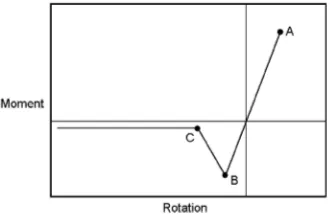
Fig. 2 Moment-rotation relationship for a two-dimensional tape-spring fold.

be folded elastically.4 _{They do not require any lubrication and}

automatically lock in the deployed configuration. In recent years there has been committed research into the use of tape springs in de-ployable structures.5_{Such work has focused on tape springs folded}

in two dimensions, as shown in Fig. 1 (folded throughθdeg). This research has resulted in the development of hinge systems such as the tape-spring rolamite hinge6 _{(developed by the Deployable}

Structures Lab in Cambridge, England, United Kingdom) and the French low-cost tape spring hinge7_{[developed by Centre National}

d’Etudes Spatiales/METRAVIB RDS on behalf of the Centre Na-tional d’Etudes Spatiales/Detection of Electro-Magnetic Emissions Transmitted from Earthquake Regions (DEMETER) program].

When a tape spring of length L is loaded by equal and opposite applied moments M, in the soft plane of the tape spring a standard moment-rotation relationship is produced as shown in Fig. 2. Buck-ling occurs at A and B (known as the peak moments), after which localized folds form in the tape spring. The reaction moments of the tape spring then remain approximately constant. These constant moments are known as steady-state moments (M₊∗and M₋∗).

This moment-rotation relationship is the basis of two-dimensional tape-spring bend analysis, which predicts the peak moments (Mmax

+ ,

Mmax

− ) and the steady-state moments (M+∗, M−∗). It is defined that

positive applied moments produce tension along the edges of the strip, resulting in a longitudinal curve that is in the opposite sense to the initial transverse curve of the tape spring. This is known as an opposite-sense bend. Conversely, negative applied moments create compression along the edges of the strip, resulting in an equal-sense bend.5_{Opposite sense bends buckle via a snap-through mode}

(point A; Fig. 2), whereas equal-sense bends buckle via a torsional mode (point B; Fig. 2). This means that opposite-sense peak mo-ments are higher than equal-sense peak momo-ments.

Three-dimensional tape-spring folds not only incorporate lon-gitudinal bending but also twisting of the tape. The relative twist angle between the ends of the tape spring is denoted byγ. A simple three-dimensional fold can be seen in Fig. 3. Such a fold is formed whenever the fold line is not perpendicular to the axis of the tape (Fig. 4). Therefore, if the tape spring is not mounted perpendicularly to the deployment appendage a three-dimensional fold will be cre-ated. If the true fold line is at 45 deg to the two-dimensional fold line, then a right-angle three-dimensional fold is created. This results in a final fold ofθ=90 deg andγ=180 deg (as shown in Fig. 3). A “perfect” fold path, used for all experimental and theoretical static tests, is defined as a path that has a constant relationship between θandγ. Therefore, a right-angle three-dimensional fold follows a perfect fold path defined byγ=2θ.

Fig. 3 Three-dimensional tape-spring fold.

Fig. 4 Fold line overlaid on a tape spring.

Fig. 5 Initial coordinate system.

Future deployment designs that incorporate three-dimensional folds have been presented in previous studies.8 _{In fact there are}

specific advantages in using angled tape springs to deploy panels, such as a thinner packing thickness if the tape springs are mounted on the upper and lower panel surface (increasing the stiffness of the hinge). Such advantages could lead to many future applications of this concept. It is therefore necessary to perform some initial investigations into the deployment dynamics of such systems.

III. Static Analysis of Three-Dimensional Tape-Spring Folds

To perform a theoretical analysis of the tape spring, it is first necessary to define a suitable coordinate system. Because of the nature of the displacement, two coordinate systems are required to describe the motion of the tape. The first is displayed in Fig. 5. Axes

x, y, and z are a fixed co-ordinate system in relation to the initial

unfolded length of tape. The dashed axes shown in Fig. 6 denote a moving coordinate system that stays in the flat plane of the tape spring as shown. Longitudinal bending occurs around the y axis, and twisting occurs around the xaxis.

Using shell theory mathematics, Mansfield9 _{derived the}

Fig. 6 Rotating coordinate system.

plot: ¯

M= ¯κx− ¯κx,0+[λ/(1−ν2)][µ1(κ¯x)−λκ¯x2(κ¯x)] (1)

where

µ=2νκ¯x− ¯κy,0−νκ¯x,0 (2)

λ= ¯κ2 x y− ¯κ

2

x y,0+(¯κx− ¯κx,0)(νκ¯x− ¯κy,0) (3)

1(¯κx)=

1 ¯ κ2 x     1−

1 ¯ κ12

x

  cosh

2κ¯

1 2

x −cos

2κ¯

1 2

x

sinh

2κ¯

1 2

x +sin

2κ¯

1 2 x         (4)

2(¯κx)=

1 ¯ κ4 x     1+

sinh

2κ¯

1 2

x sin

2κ¯

1 2 x sinh 2κ¯

1 2

x +sin

2κ¯

1 2

x 2

− 5 4κ¯

1 2 x    cosh

2κ¯

1 2

x −cos

2κ¯

1 2

x

sinh

2κ¯

1 2

x +sin

2κ¯

1 2 x         (5)

Equation (1) essentially states thatM¯= f(κ¯x), which is the

equiv-alent of M=f(θ)(Ref. 5). Nondimensional values of the longitu-dinal moment and the curvatures are used (denoted by M and¯ κ¯, respectively) to avoid indeterminate expressions in the main equa-tion. These nondimensional parameters are found using Eqs. (6) and (7):

¯

M=

3a[3(1−ν2_)]1₂ Et4

M (6)

{¯κx,0,κ¯x y,0,κ¯y,0,κ¯x,κ¯x y}

= a2[3(1−ν2)]

1 2

4t {κx,0, κx y,0, κy,0, κx, κx y} (7) There is an equivalent equation for the tape-spring reaction torque, as shown in Eq. (8). This is a function of two curvature variables

¯

T= f(κx, κx y), which is the equivalent of T= f(θ, γ ):

¯

T= ¯κx y− ¯κx y,0+

λκ¯x y1(¯κx)

1−ν (8)

¯

T=

3a[3(1−ν2_)]1₂

4Gt4

T (9)

From analytical studies of three-dimensional surface curvatures, it is known that a three-dimensional surface is defined by two lines of principle curvature, which are perpendicular to each other.10_These

are the lines of maximum and minimum curvature of the surface. If this is applied to the postbuckling analysis of tape springs, it can be seen that as twist is applied to the tape the lines of principle curvature rotate (Fig. 7). The angle of this rotation is signified by the change inφ. This rotation ofφimpacts the surface curvature matrix as shown in Eq. (10), whereλ1andλ2are the maximum and

minimum curvatures of the surface, respectively:

λ2,κxcan be recalculated. Using Eqs. (7), (1), and (6), a value for

the longitudinal reaction moment can then be found. This solution, however, does not take into account the length of the tape spring (hence the resultant rotation of the flat strips on either side of the central fold). To include this in the analysis, the theoretical tape model was divided into three segments as shown in Fig. 8. Because of the symmetry of the model, segments 1 and 3 are assumed to be identical. The twist of these segments is calculated using stan-dard torsion theory.11_{The resultant torque from these segments is}

balanced with the reaction torque from segment 2 [Eq. (11)]: ¯

κx y− ¯κx y,0+λκ¯x y1(κ¯x)/(1−ν)

3a[3(1−ν2)_]124Gt4

= G J

L−ls2

(γ−γ2) (11)

The length of the central segment ls2 is a key parameter in this

equation. A correct value of ls2would result inφ=45 deg when

γ=180 deg. A low value of ls2would result in high curvatures in

the fold region, and a high value of ls2would result in a low value

ofφwhenγ=180 deg. This parameter is specific to the sectional and material properties of the specimen and was determined exper-imentally. Because of all straight tape rotation being in segments 1 and 3, it can be assumed that a linear relationship exists betweenγ2

andφ.γ2can therefore be approximated using Eq. (12):

γ2=4φ (12)

This calculation process, shown in Fig. 9, outputs the resultant ro-tation of the principle curvature linesφ, which in turn allows the bending and twisting reaction moments to be calculated. This the-oretical analysis was implemented with the parameters in Table 1

Table 1 Properties of experimental tape-spring cross sectiona

Parameter Value

E 205×103_Nmm

ν 0.3

α 1.25 rad

tts 0.11 mm

Ry 20 mm

κy,0 0.05

κx,0 0

D 24.99 Nmm4

L 400 mm

ls2 344 mm

a_{All values determined experimentally except E andν.}

a) b)

Fig. 7 Rotation of the lines of principle curvature.

Fig. 9 Calculation process.

Fig. 10 Experimental test rig.

Fig. 11 Bending reaction moment results.

and compared with experimental test results of a right-angle three-dimensional tape-spring fold following a perfect fold path. (The experimental test rig is shown in Fig. 10.) The analytical results, overlayed on the experimental results, can be seen in Fig. 11 (for the bending moment M) and Fig. 12 (for the twisting moment T ). It was found that if two critical tape parameters (the torsional stiffness of segments 1 and 3 and the length of segment 2) were determined accurately, then the theoretical model would closely model the ex-perimental result. It was found that the presence of an incrementing twist angle in the fold causes the longitudinal steady-state moment to rise. This, in turn, would have an impact on the deployment dy-namics of three-dimensional bends compared to two-dimensional bends.

IV. Initial Dynamic Model Predictions

Dynamic modeling of two-dimensional tape springs has been previously performed in order to study the deployment dynamics of simple composite panels.12_{The full model for the deployment of an}

equal sense, two-dimensional tape-spring fold is based on the mod-eled moment rotation plot shown in Fig. 13, where the coordinates of the critical points can be calculated from both analytical

expres-Fig. 12 Twisting reaction moment results.

Fig. 13 Moment rotation plot for two-dimensional equal-sense bend deployment.

sions (derived by W¨ust13_{and Rimrott}14_{) and polynomial functions}

(derived by Seffen et al.12_{) within reasonable accuracy limits.}

In this current work the tape is modeled as a simple hinge in order to study the impact of the steady-state moment rise on the system dynamics, as this is the largest time segment of the tape-spring deployment [especially ifθ(at t=0)=180 deg]. If a tape spring is subjected to a three-dimensional fold whereγ=180 deg andθ <90, then the principal curvature lines become increasingly overrotated asθreduces. This can result in high curvatures, hence high stresses in the fold region, making these folds unattractive for any practical use. Therefore only right-angle three-dimensional folds following a perfect fold path will be studied as this is the worst practical case for the effect of twist on the bending moment. The prebuckling moment-rotation relationship is assumed to be equivalent to the two-dimensional model because of the relative small angles ofθ involved.

By linearly interpolating the result of the postbuckling analyti-cal model, a simple relationship was found between M andθ(for θ >14.6 deg), shown in Eq. (13), whereθis measured in radians,

mA=0.0102, and mB=0.0188:

M=mAθ+mB (13)

M=Iyθ¨ (14)

A simple dynamic model11 _{can then be created by substituting}

Eq. (13) into Eq. (14). The moments of inertia about the x and

y axes were calculated as a number of small lumped masses, at

increasing lengths from the fold point. Equation (14) can then be rearranged into Eq. (15), which is the standard format for a linear, second-order, differential equation with known constant coefficients (mC=mA/I y and mD=mB/I y) and no damping:

¨

θ+mCθ= −mD (15)

Solving Eq. (15) with the boundary conditions θ(0)=π/2 and ˙

Fig. 14 Displacement deployment model of tape spring.

Fig. 15 Angular velocity deployment model of tape spring.

where

λi=

√

mC, Cm= −mD/mC

Bm=0, Am=π/2−Cm (17)

The overall solution can be seen in Fig. 14 (denoted byθ1), overlayed

on the two-dimensional result (denoted byθ2), with a steady-state

moment of−21.86 Nmm. It can be seen that the steady-state moment rise has shortened the deployment time by 18%, and from Fig. 15 the angular velocity before snap back (point C; Fig. 13) has increased by 13.5%.

After the tape spring snaps back to its initial state, it can be seen from both Figs. 14 and 15 that rapid oscillations occur. This high-frequency motion is caused by the tape spring oscillating between points A and B in Fig. 13. With no damping these restoring motions and resultant velocity changes continue for all larger values of t. Such motion is beyond the scope of this study.

Referring back to Fig. 14, it can be seen that there is also an overlay ofγ for the twisting dynamics of the deployment. This is calculated using a similar expression as Eq. (13) but without the constant term (as zero twist results in zero reaction torque) where

mA=0.0036. The two independently calculated dynamic results

(θ1andγ) suggest that because of the low inertia of the tape about

the xaxis the tape twists by just under 1.5 oscillations before the snap back. For an undamped, theoretical model of a tape spring released in free space, this can be a representative result. However, from experimental testing it is clear that for any practical purpose (involving tape spring fixings and attachments) this does not occur.

Fig. 16 Realistic system layout.

Fig. 17 Area deployment.

If a more realistic system (shown in Fig. 16), where one end of the tape spring is fixed in space and the other is moved to form a right-angle three-dimensional fold (θ=90 deg,γ=180 deg), is considered, then from experimental observations the nature of the dynamics is very different from those of this theoretical model. It can be concluded from experimental observations that there are three primary stages for the deployment of a three-dimensional fold in this configuration. The first stage, once released, is the rapid twist correction of the free half of the spring, with little comparative oscillations. This is because oscillations beyond this zero twist point would result in high twist reaction moments from the fold (currently twisted in the opposite sense). The second stage is the longitudinal unfolding of the tape spring. Any twist remaining is over the tape length between the fold and the fixed end. The impact of this on the longitudinal deployment is related to the way the tape is fixed and the length of the tape from the fixed end to the fold. If the fold is well outside the region of end effects (created by the fixed end), then asθreduces the fold will move toward the fixed end. The final stage is the lowθ snap back, followed by twist oscillations. If the momentum of the spring is large enough, the tape spring “bounces” out and buckles the tape in the opposite direction of twist. Note that this is the equivalent of the two-dimensional fold snap through, which is a sign change inθ, as apposed to this three-dimensional case, which is a sign change inγ.

V. Dynamics of Array Deployment

The true deployment nature of tape springs folded in three di-mensions is clearly very complex and very specific to the system in which they are incorporated. Therefore to proceed further it is necessary to apply the dynamic models to a specific deployment system. Further analysis will focus on the stage two deployment of a simply supported area deployment device (as presented in Walker and Aglietti8_{). This design incorporates two, three-dimensionally}

folded tape springs, which deploy to support an array fabric as shown in Fig. 17 (where the thick dotted lines denote the tape springs). Although the preceding simple dynamic model concluded that, in general, realistic three-dimensional tape-spring deployments do not follow the perfect fold path, it can be assumed for this application that the tape springs do follow this path because of the constraints of the array attachments.

Fig. 18 Variables for analysis 1.

Fig. 19 Variables for analysis 2.

Fig. 20 Variables for analysis 3.

The three critical angles in this analysis areµ(Fig. 18),(Fig. 19 which also defines), andβ(Fig. 20). The hinge moment around the fold line is then the sum of the resolved twist and bending moments, where the bending moment is a function ofθand the twist moment is a function ofγ [as shown in Eq. (18)]:

Mhinge=M(θ)sinβcosµ+T(γ )sinµ (18)

γ can be simply determined using the relationship γ=180−. However, to determineθit is first necessary to determine the angle βin terms of andµ. This has to be performed separately for ≤90 deg and≥90 deg:

For≤90 deg,

β=tan−1

l1sin l2cosµ+l1cossinµ

(19)

For≥90 deg, if

ε=−90 (20)

then

β=tan−1

l1cosε l2cosµ−l1sinεsinµ

(21)

If≥90 deg, thenθcan be found using Eq. (22): θ=sin−1

2l1sin

L sinβ

(22) If, however,≤90 deg andµ≤45 deg (i.e.,θin the undeployed configuration is greater than 90 deg) then initiallyσ (the internal angle between both longitudinal halves of the tape spring) must be determined beforeθcan be calculated.

So for≤90 deg, ifµ≤45 deg andσ≤90 deg then σ =sin−1

2l1sin

L sinβ

(23) Therefore

θ=180−σ (24)

This method is used untilσ=90 deg, after whichθ can then be calculated directly using Eq. (25):

So for≤90 deg,σ≥90 deg, θ=sin−1

2l1sin

L sinβ

(25) The values for this analysis are shown in Table 2. Mhingewas then

determined for the deployment using the static analysis method and Eqs. (18), (19), (21), and (22). This resulted in a moment rotation relationship up toθ=14.6 deg, as shown in Fig. 21. Here it can be seen that the initial hinge moment (dominated by the torque) is low. The moment magnitude is also lower throughout the deployment than the steady-state moment for a two-dimensional fold.

Using the inertial properties of the array, a dynamic model was created. The displacement dynamics and angular velocity results are shown in Figs. 22 and 23, respectively. It can be seen that (without

Table 2 Properties of array

Parameter Value

L 0.8485 m

l1, l2 0.3 m

µ 45 deg

Iarray 9.525×10−3kgm2

Fig. 21 Moment-rotation relationship for array.

Fig. 23 Angular velocity deployment model of array.

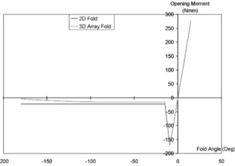
Fig. 24 Full moment rotation plot two-dimensional tape spring and three-dimensional array fold.

damping) the deployment time has increased to just under 2 s and the angular velocity just before snap back is much lower than the free tape spring, as expected. By applying an energy method,12 _a

prediction can be made as to whether the tape spring, without damp-ing, will snap through forming an opposite-sense fold. The method compares the area under the moment-rotation curve to the left of the vertical axis with the area under the curve on the right of the vertical axis. Figure 24 displays both the two-dimensional system and the equivalent three-dimensional system. It was found that the unfolding energy of the two-dimensional system was 2.368 times greater than the threshold energy necessary to cause snap through. The equivalent three-dimensional system shows that (because of the low initial moments about the hinge) the deployment energy has re-duced significantly to 1.678 times the threshold energy. Although a snap through is still predicted to occur, the energy available to cause the snap though has been halved. Therefore, not only is the deployment slower, but also less damping is required in the system to prevent snap through.

ment application. The static reaction moments produced by a three-dimensional tape-spring fold can be determined using shell theory mathematics, three-dimensional surface mathematics, and standard torsion theory. Using simple dynamic models, the undamped dy-namic behavior of a tape spring in free space could easily be de-termined. By deriving a set of equations to determine the impact of the tape-spring moments on the hinge or fold line of an array, these methods could then applied to a specific deployment applica-tion. It was found that, compared to the two-dimensional case, the deployment was slower (reaching much lower angular velocities) and the deployment energy of the system was significantly reduced, thus making it easier to prevent a snap through of the tape springs. This, in turn, would reduce the damping required in the system, and hence reduce the mass of the array.

References

1_{Bishop, D., Giles, R., and Austin, G., “The Lucent LambdaRouter:}

MEMS Technology of the Future Here Today,” IEEE Communications

Mag-azine, 2002, Vol. 40, No. 3, pp. 75–79.

2_{Paine, M., and Gabriel, S., “A Micro-Fabricated Colloidal Thruster}

Ar-ray,” AIAA Paper 2001-3329, July 2001.

3_{Simburger, E., Matsumoto, J., Lin, J., Rawal, S., Peterson, T., and}

Kerslake, T., “Development of a Multifunctional Inflatable Structure for the PowerSphere Concept,” AIAA Paper 2002-1707, April 2002.

4_{Seffen, K. A., You, Z., and Pellegrino, S., “Folding and Deployment}

of Curved Tape Springs,” International Journal of Mechanical Sciences, Vol. 42, 2000, pp. 2055–2073.

5_{Seffen, K. A., and Pellegrino, S., “Deployment Dynamics of Tape}

Springs,” Proceeding of the Royal Society of London, Vol. A 455, 1999, pp. 1003–1048.

6_{Watt, A. M., and Pellegrino, S., “Tape-Spring Rolling Hinges,” NASA}

CP-2002-211506, May 2002.

7_{Givois, D., Sicre, J., and Mazoyer, T., “A Low Cost Hinge for Appendices}

Deployment: Design, Test and Applications,” 9th European Space Mecha-nisms and Tribology Symposium, ESA/ESTEC, Sept. 2001.

8_{Walker, S. J. I., and Aglietti, G., “An Application of Tape Springs in}

Small Satellite Area Deployment Devices,” Proceedings of 5th International

Conference on Dynamics and Control of Systems and Structures in Space,

edited by T. S. Bowling and R. L. Oswald, Cranfield Univ. Press, Cranfield, England, U.K., 2002, pp. 131–137.

9_{Mansfield, E. H., “Large-Deflection Torsion and Flexure of Initially}

Curved Strips,” Proceedings of the Royal Society of London, Vol. A 334, 1973, pp. 279–298.

10_{Gray, A., Modern Differential Geometry of Curves and Surfaces, CRC}

Press, Boca Raton, FL, 1993, pp. 270, 271.

11_{Megson, T. H. G., Aircraft Structures for Engineering Students, 2nd ed.,}

Edward Arnold, London, 1990, pp. 264–266.

12_{Seffen, K. A., Pellegrino, S., and Parks, G. T., “Deployment of a Panel}

by Tape-Spring Hinges,” Proceedings of IUTAM-IASS Symposium on

De-ployable Structures: Theory and Applications, 1998, pp. 355–364.

13_{W¨ust, W., “Einige Andvendungen der Theorie der Zylinderschale,”}

Zeitschrift Angewandte Mathematik und Mechanik, Vol. 34, 1954,

pp. 444–454.

14_{Rimrott, F., “Storable Tubular Extendible Members,” Engineering}

Digest, Sept. 1966.

B. Sankar