General Upper Bounds on the Runtime of Parallel Evolutionary Algorithms

White Rose Research Online URL for this paper:

http://eprints.whiterose.ac.uk/98934/

Version: Accepted Version

Article:

Lässig, J. and Sudholt, D. orcid.org/0000-0001-6020-1646 (2014) General Upper Bounds

on the Runtime of Parallel Evolutionary Algorithms. Evolutionary Computation, 22 (3). pp.

405-437. ISSN 1063-6560

https://doi.org/10.1162/EVCO_a_00114

[email protected] Reuse

Unless indicated otherwise, fulltext items are protected by copyright with all rights reserved. The copyright exception in section 29 of the Copyright, Designs and Patents Act 1988 allows the making of a single copy solely for the purpose of non-commercial research or private study within the limits of fair dealing. The publisher or other rights-holder may allow further reproduction and re-use of this version - refer to the White Rose Research Online record for this item. Where records identify the publisher as the copyright holder, users can verify any specific terms of use on the publisher’s website.

Takedown

If you consider content in White Rose Research Online to be in breach of UK law, please notify us by

J ¨org L¨assig

University of Applied Sciences Zittau/G ¨orlitz, Germany

Dirk Sudholt

Department of Computer Science, University of Sheffield, United Kingdom

Abstract

We present a general method for analyzing the running time of parallel evolutionary algorithms with spatially structured populations. Based on the fitness-level method, it yields upper bounds on the expected parallel running time. This allows to rigorously estimate the speedup gained by parallelization. Tailored results are given for common migration topologies: ring graphs, torus graphs, hypercubes, and the complete graph. Example applications for pseudo-Boolean optimization show that our method is easy to apply and that it gives powerful results. In our examples the performance guaran-tees improve with the density of the topology. Surprisingly, even sparse topologies like ring graphs lead to a significant speedup for many functions while not increasing the total number of function evaluations by more than a constant factor. We also identify which number of processors lead to the best guaranteed speedups, thus giving hints on how to parametrize parallel evolutionary algorithms.

Keywords

Parallel evolutionary algorithms, runtime analysis, island model, spatial structures

1

Introduction

Due to the increasing number of CPU cores, exploiting possible speedups by parallel computations is nowadays more important than ever. Parallel evolutionary algorithms (EAs) form a popular class of heuristics with many applications to computationally expensive problems [29, 31, 46]. This includesisland models, also calleddistributed EAs, multi-deme EAsorcoarse-grained EAs. Evolution is parallelized by evolving subpopu-lations, calledislands, on different processors. Individuals are periodically exchanged in a process calledmigration, where selected individuals, or copies of these, are sent to other islands, according to a migration topology that determines which islands are neighboring. Also more fine-grained models are known, where neighboring subpopu-lations communicate in every generation, first and foremost incellular EAs[46].

By restricting the flow of information through spatial structures and/or infrequent communication, diversity in the whole system is increased. Researchers and practition-ers frequently report that parallel EAs speed up the computation time, and at the same time lead to a better solution quality [29].

Despite these successes, a long history [5] and very active research in this area [2, 29, 39], the theoretical foundation of parallel EAs is still in its infancy. The im-pact of even the most basic parameters on performance is not well understood [41].

Past and present research is mostly empirical, and a solid theoretical foundation is missing. Theoretical studies are mostly limited to artificial settings. In the study of takeover times, one asks how long it takes for a single optimum to spread throughout the whole parallel EA, if the EA uses only selection and migration, but neither muta-tion nor crossover [38, 39]. This gives a useful indicator for the speed at which com-munication is spread, but it does not give any formal results about the running time of evolutionary algorithms with mutation and/or crossover.

One way of gaining insight into the capabilities and limitations of parallel EAs is by means of rigorous running time analysis [15, 47]. By asymptotic bounds on the running time we can compare different implementations of parallel EAs and assess the speedup gained by parallelization in a rigorous manner. Many running time analyses have been presented [4, 18, 34, 35], from simple pseudo-Boolean test functions [8] to NP-hard problems from combinatorial optimization [9, 17, 48, 50].

In [23] the authors presented the first running time analysis of a parallel evo-lutionary algorithm with a non-trivial migration topology. It was demonstrated for a constructed problem that migration is essential in the following way. A suitably parametrized island model with migration has a polynomial running time while the same model without migration as well as comparable panmictic populations1_need ex-ponential time, with overwhelming probability. Neumann, Oliveto, Rudolph, and Sud-holt [32] presented a similar result for island models using crossover. If islands perform crossover with immigrants during migration, this can drastically speed up optimiza-tion. This was demonstrated for a pseudo-Boolean example as well as for instances of the VERTEXCOVERproblem [32].

In this work we take a broader view and consider the speedup gained by paral-lelization in terms of the number of generations, for various common pseudo-Boolean functions and function classes of varying difficulty. A general method is presented for proving upper bounds on the parallel running time of parallel EAs. The latter is de-fined as the number of generations of the parallel EA until a global optimum is found for the first time. This allows us to estimate the speedup gained by parallelization, defined as the ratio of the expected parallel running time of a single island and the ex-pected running time of an island model with multiple islands (see Section 2 for formal definitions). It also can be used to determine how to choose the number of islands such that the best possible upper bounds on the parallel running time are obtained, while still maintaining an asymptotically optimal speedup.

Our method is based on the fitness-level methodor method off-based partitions, a simple and well-known tool for the analysis of evolutionary algorithms [8, 47]. The main idea of this method is to divide the search space into sets A1, . . . , Am, strictly

ordered according to fitness values of elements therein. Elitists EAs, i. e., EAs where the best fitness value in the population can never decrease, can only increase their current best fitness. If, for each setAi we know a lower boundsi on the probability that an

elitist EA finds an improvement, i. e., for finding a new search point in a new best fitness-level set Ai+1∪ · · · ∪Am, this gives rise to an upper bound Pmi=11/si on the

expected running time. The method is described in more detail in Section 2.

In Section 3 we first derive a general upper bound for parallel EAs, based on fitness levels. Our general method is then tailored towards different spatial structures often used in fine-grained or cellular evolutionary algorithms and parallel architectures in general: ring graphs (Theorem 8 in Section 4), torus graphs (Theorem 10 in Section 5),

hypercubes (Theorem 12 in Section 6) and complete graphs (Theorems 14 and 17 in Section 7).

The only assumption made is that islands run elitist algorithms, and that in each generation each island has a chance of transmitting individuals from its best current fit-ness level to each neighboring island, independently with probability at leastp. We call the latter thetransmission probability. It can be used to model various stochastic effects such as disruptive variation operators, the impact of selection operators, probabilistic migration, probabilistic emigration and immigration policies, and transient faults in the network. This renders our method widely applicable to a broad range of settings.

1.1 Main Results

Our estimates of parallel running times from Theorems 8, 10, 12, 14, and 17 are sum-marized in the following theorem, hence characterizing our main results. Throughout this workµalways denotes the number of islands.

Theorem 1. Consider an island model withµislands where each island runs an elitist EA. For each island let there be a fitness-based partitionA1, . . . , Amsuch that for all1 ≤ i < mall

points inAi have a strictly worse fitness than all points inAi+1, andAmcontains all global

optima. We say that an island is inAiif the best search point on the island is inAi. Letsibe a

lower bound for the probability that in one generation a fixed island inAifinds a search point

inAi+1∪ · · · ∪Am.

Further assume that for each edge in the migration topology in every iteration there is a probability of at leastpthat the following holds, independently from other edges and for all1≤

i < m. If the source island is inAithen after the generation the target island is inAi∪· · ·∪Am.

Then the expected parallel running time of the island model is bounded from above by

1. O

1

p1/2 Pm−1

i=1 1

s1i/2

+_µ1Pm−1

i=1 1

si for every ring graph or any other strongly connected 2

topology (Theorem 8),

2. O

1

p2/3 Pm−1

i=1 _s11/3

i

+_µ1Pm−1

i=1 s1i for every undirected grid or torus graph whose side

lengths are at leastõin both directions (Theorem 10),

3. Om+Pmi=1−1log(1/si) p

+1

µ

Pm−1

i=1 s1i for the(logµ)-dimensional hypercube graph

(Theo-rem 12),

4. O(m/p) +1

µ

Pm−1

i=1 s1i for the complete topologyKµ, as well as Om+_minm_{log_pµ,µ_1}+1

µ

Pm−1

i=1 s1i (Theorems 14 and 17).

A remarkable feature of our method is that it can automatically transfer upper bounds for panmictic EAs to parallel versions thereof. The only requirement is that bounds on panmictic EAs have been derived using the fitness-level method, and that the partition A1, . . . , Am and the probabilities for improvements s1, . . . , sm−1 used

therein are known. Then the expected parallel time of the corresponding island model can be estimated for all mentioned topologies simply by plugging thesi into

Theo-rem 1. Fortunately, many published runtime analyses use the fitness-level method— either explicitly or implicitly—and the mentioned details are often stated or easy to

2_{A directed graph is strongly connected if for each pair of vertices}

derive. Hence even researchers with limited expertise in runtime analysis can easily reuse previous analyses to study parallel EAs.

Further note that we can easily determine which choice ofµ, the number of is-lands, will give an upper bound of order1/µ·Pm−1

i=1 1/si—the best upper bound we

can hope for, using the fitness-level method. In all bounds from Theorem 1 we have a first term that varies with the topology and p, and a second term that is always

1/µ·Pm−1

i=1 1/si. The first term reflects how quickly information about good fitness

levels is spread throughout the island model. Choosingµsuch that the second term becomes asymptotically as large as the first one, or larger, we get an upper bound of

O1/µ·Pm−1

i=1 1/si

. For settings where Pm−1

i=1 1/si is an asymptotically tight upper

bound for a single island, this corresponds to an asymptotic linear speedup. The max-imum feasible value forµdepends on the problem, the topology and the transmission probabilityp.

(1+1) EA Ring Grid/Torus Hypercube Complete

OneMax

bestµ µ= Θ(logn) µ= Θ(logn) µ= Θ(logn) µ= Θ(logn)

E(Tpar) Θ(nlogn) Θ(n) Θ(n) Θ(n) Θ(n)

E(Tseq_{) Θ(nlogn) Θ(nlogn) Θ(nlogn) Θ(nlogn) Θ(nlogn)}

E(Tcom_{) 0 Θ(nlogn) Θ(nlogn) Θ(n(logn) log logn) Θ(nlog}2_n)

LO

bestµ µ= Θ(n1/2_{) µ= Θ(n}2/3_{) µ= Θ} n

logn

µ= Θ(n)

E(Tpar_{) Θ(n}2_{) Θ(n}3/2_{) Θ(n}4/3_{) Θ(nlogn) Θ(n)}

E(Tseq_{) Θ(n}2_{) Θ(n}2_{) Θ(n}2_{) Θ(n}2_{) Θ(n}2₎

E(Tcom_{) 0 Θ(n}2_{) Θ(n}2_{) Θ(n}2_log2_{n) Θ(n}3₎

unimodal

bestµ µ= Θ(n1/2_{) µ= Θ(n}2/3_{) µ= Θ} n

logn

µ= Θ(n)

E(Tpar_{) O(dn) O dn}1/2

O dn1/3

O(dlogn) O(d)

E(Tseq_{) O(dn) O(dn) O(dn) O(dn) O(dn)}

E(Tcom_{) 0 O(dn) O(dn) O(dnlogn) O dn}2

Jump

kbestµ µ= Θ(n

k/2_{) µ= Θ(n}2k/3_{) µ= Θ(n}k−1_{) µ= Θ(n}k−1₎

E(Tpar_{) Θ(n}k_{) O n}k/2

O nk/3

O(n) O(n)

E(Tseq_{) Θ(n}k_{) O n}k

O nk

O nk

O nk E(Tcom_{) 0 O n}k

O nk

O knk_logn

O n2k−1

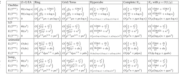
Table 1: Asymptotic bounds on expected parallel (Tpar_{, number of generations) and}

sequential (Tseq_{, number of function evaluations) running times and expected}

commu-nication efforts (Tcom_{, total number of migrated individuals) for variousn-bit functions}

and island models withµislands running the (1+1) EA and using migration probabil-ityp= 1. The number of islandsµwas always chosen to give the best possible upper bound on the parallel running time, while not increasing the upper bound on the se-quential running time by more than a constant factor. For unimodal functionsd+ 1

denotes the number of function values. See [8] for bounds for the (1+1) EA. Results for Jump_kwere restricted to3 ≤k=O(n/logn)for simplicity. All upper bounds for OneMax and LO stated here are asymptotically tight, as follows from general results in [43].

each island (see Section 2 for details). Table 1 summarizes the resulting running time bounds for the considered algorithms and problem classes. For simplicity we assume

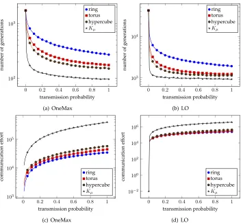
p= 1; a more detailed table for general transmission probabilities is presented in the appendix, see Table 3. The number of islandsµwas chosen as explained above: to give the smallest possible parallel running time, while not increasing the sequential time, asymptotically. The table also shows the expectedcommunication effort, defined as the total number of individuals migrated throughout the run. Details are given in Theo-rems 8, 10, 12, 14, and 17. Bounds on the expected communication effort follow easily from bounds on the parallel running time using Theorem 2. The functions used in this table are explained in Section 2. Table 3 in the appendix shows all our results for a variable number of islandsµand variable transmission probabilitiesp.

The method has already found a number of applications and it spawned a number of follow-up papers. After the preliminary version of this work [24] was presented, the authors applied it for various problems from combinatorial optimization: the sorting problem (as maximizing sortedness), finding shortest paths in graphs, and Eulerian cy-cles [26]. Very recently, Mambrini, Sudholt, and Yao [30] also used it for studying how quickly island models find good approximations for the NP-hard SETCOVERproblem. This work has also led to the discovery of simple adaptive schemes for changing the number of islands dynamically throughout the run, see L¨assig and Sudholt [25]. These schemes lead to near-optimal parallel running times, while asymptotically not increas-ing the sequential runnincreas-ing time on many examples [25]. These schemes are tailored to-wards island models with complete topologies, which includes offspring populations as special case. The study of offspring populations in comma strategies is another re-cent development that was inspired by this work [37].

2

Preliminaries

We are interested in the following performance measures, where the number of islands,

µ, in the considered island model is obvious from the context. First we define the parallel running timeTparas the number of generations until the first global optimum is evaluated. LetTµbe the number of generations before the island model finds a global

optimum for the first time. Then

Tpar_:=T

µ.

Thesequential running timeTseq _{is defined as the number of function evaluations}

un-til the first global optimum is evaluated. It thus captures the overall effort across all processors. It is formally defined as

Tseq :=µ·Tµ.

In both measuresTparandTseqwe allow ourselves to neglect the cost of the initializa-tion as this only adds a fixed term to the running times.

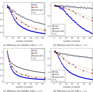
Thespeedupis defined as the ratio of expected running times of a single island and an island model withµislands:

E(T1)/E(Tµ).

Our definition of speedup is calledweak orthodox speedupin Alba’s taxonomy [1]. If the speedup is at least of order µ, i. e., if it isΩ(µ), we speak of alinear speedup. In this work it is generally understood in an asymptotic sense, unless we call it aperfect linear speedup.

global optimum, the execution time of an island model withµislands can be estimated as

Execµ=Tµ·(Execgenµ + Exec

migr

µ ) (1)

where Execgen is the execution time for one generation (excluding migration) and

Execmigr is the execution time for migration. The latter depends on the number of islands, the communication topology, and the number of individuals migrated. For sequential algorithms (µ = 1) we have Execmigr1 = 0. Contrarily, for homogeneous

parallel systems we may assume thatExecgenµ is fixed, that is, independent ofµ.

Many common definitions of “speedup” consider the wall-clock time, where the differences inExecmigrplay a role. Here we consider speedups with regard to the num-ber of generations only, ignoring the differences inExecmigr. This makes sense in setting whereExecgen≫Execmigr; for instance, when fitness evaluations are so expensive that they dominate the execution time. Otherwise, the speedups stated here may be op-timistic as the overhead induced by migration is ignored. Note, however, that with additional information aboutExecgenandExecmigrand Equation (1) our results easily extend to more sophisticated notions of speedups.

To get a more complete picture of the resources used in a parallel system and to take into account the overhead by communication, we also consider the communica-tion effortTcom_{. It is defined as the total number of individuals migrated to other}

is-lands during the course of a run. The communication effort therefore captures the total bandwidth used during a run of an island model. It represents an important factor for determining the performance of a parallel EA, alongside the parallel running time.

The expected communication effort is a multiple of the parallel expected running time, with the factor depending on the number of (directed) edges in the topology, the transmission probabilitypand the number of individuals migrated in each migration event.

The following theorem lists various topologies: a unidirectional ring is a graph consisting of a single directed cycle, whereas a directed ring has undirected edges. Note that an undirected edge can be regarded as two directed edges. In a torus graph all ver-tices are arranged on a two-dimensional grid, with undirected edges wrapping around (vertices in the top row are neighbored to the ones in the bottom row and vice versa, similarly for the leftmost and rightmost columns). Each vertex in a torus thus has 4 distinct neighbors, provided that the torus has at least 3 rows and at least 3 columns. Hypercubes are formally defined in Section 6, and the complete graph Kµ contains

undirected edges between all pairs of nodes.

Theorem 2. Consider an island model with a directed graphT = (V, E)as topology, such that in each generation along each directed edge migration takes place independently with probabil-ityp. Assume thatν individuals are migrated in each migration event. LetTpar_{be the parallel}

running time of the island model, then the expected communication effort E(Tcom)is

E(Tcom) =pν· |E| ·E(Tpar). (2)

Thereby, if|V|=µ, we have

• |E|=µfor a unidirectional ring and|E|= 2µfor a bidirectional ring,

• |E|= 4µfor any torus graph where both sides have length at least3,

• |E|=µlogµfor the(logµ)-dimensional hypercube, and

Proof. Fix a single edgee, then the expected number of migration events acrosseequals

∞

X

t=0

Prob(Tpar=t)·t·p=p·E(Tpar)

by definition of E(Tpar_{). By linearity of expectations, we can add these values for all}

edges to get the expected number of migration events across the whole topology. This yields a factor of|E|. Additionally multiplying byνgives the expected communication effort.

Hence to estimate the expected communication effort it suffices to analyze the ex-pected parallel running time.

In our example applications we consider the maximization of a pseudo-Boolean functionf:{0,1}n _{→ R. It is easy to adapt the method for minimization. The}

num-ber of bits is always denoted byn. The following well known example functions have been chosen because they exhibit different probabilities for finding improvements in a typical run of an EA. For a search point x ∈ {0,1}n _{write x = x}

1. . . xn, then

OneMax(x) := Pn

i=1xi counts the number of ones inxand LO(x) := Pni=1

Qi

j=1xi

counts the number of leading ones inx, i. e., the length of the longest prefix containing only 1-bits. A function is calledunimodalif every non-optimal search point has a Ham-ming neighbor (i. e., a point with HamHam-ming distance 1 to it) with strictly larger fitness. Observe that LO is unimodal as flipping the first 0-bit results in a fitness increase. For LO every non-optimal point has exactly one Hamming neighbor with a better fitness. For1≤k≤nwe also consider

Jump_k:=

(

k+Pn

i=1xi, if

Pn

i=1xi≤n−korx= 1n,

Pn

i=1(1−xi) otherwise.

This function has been introduced by Droste, Jansen, and Wegener [8] as a function with tunable difficulty as evolutionary algorithms typically have to perform a jump to overcome a gap by flippingkspecific bits. It is also interesting because it is one of very few examples where crossover has been proven to be essential [19, 22].

Our method for proving upper bounds is based on the fitness-level method [8, 47]. The idea is to partition the search space into setsA1, . . . , Amcalledfitness levelsthat are

ordered with respect to fitness values. We say that an algorithm is inAior on leveliif

the current best individual in the population is inAi. An evolutionary algorithm where

the best fitness value in the population can never decrease (called anelitistEA) can only improve the current fitness level. If one can derive lower bounds on the probability of leaving a specific fitness level towards higher levels, this yields an upper bound on the expected running time.

Theorem 3(Fitness-level method). For two setsA, B ⊆ {0,1}n _{and a fitness functionf}

letA <f Biff(a)< f(b)for alla∈Aand allb ∈ B. Partition the search space into

non-empty setsA1, A2, . . . , Amsuch thatA1<f A2 <f · · ·<f AmandAmonly contains global

optima. For an elitist EA letsibe a lower bound on the probability of creating a new offspring

inAi+1∪ · · · ∪Am, provided the population contains a search point inAi. Then the expected

number of iterations of the algorithm to find the optimum is bounded from above by

m−1

X

i=1

1 si

In contrast to other methods such asdrift analysis[16, 21], the fitness-level method is applicable in cases where “easy” and “hard” fitness levels are mixed up, so that the progress towards the optimum cannot reasonably be bounded by a closed formula.

The fitness-level method has also been applied to other elitist optimization meth-ods, including elitist ant colony optimizers [14, 33] and a binary particle swarm opti-mizer [45]. It gives rise to powerful tail inequalities [51] and it can be used to prove lower bounds as well, when combined with additional knowledge on transition prob-abilities [43]. Finally, Lehre [27] recently showed that the fitness-level method can be extended towards non-elitist EAs with additional mild conditions on transition proba-bilities and the population size.

Note that the method only requires a finitenumberof fitness-level sets, not a finite set of fitness values. So in principle the method can be applied to continuous fitness functions as well, provided a suitable discretization is made and the goal is to find the best fitness-level set. This might not be the most practical approach, though.

In the following we apply the fitness-level method to parallel EAs. For the consid-ered EAs we assume that there is amigration topology, given by a directed graph. Islands represent vertices of the topology and directed edges indicate neighborhoods between the islands. We often describe undirected graphs for use as migration topology, un-derstanding that for an undirected edge{u, v}we have two directed edges(u, v)and

(v, u). In other words, though formally the migration topology is a directed graph, we

often use the language of undirected graphs to describe it.

Our methods for proving upper bounds require that the islands run elitist evo-lutionary algorithms. All islands create new offspring independently by mutation and/or recombination among individuals in the island. In every generation there is a chance that migration will send an individual on the current best fitness level to some target island, and that this individual will be included on the target island. This would effectively increase the fitness level of the target island to the current best level (or an even better one). For every pair of connected islands, we call this probability trans-mission probability and denote itp. Note that for any pair of islands, the mentioned transmission events are independent.

The transmission probability can model various settings, where randomness and stochasticity may be involved:

• migrations do not take place in every generation, but only probabilistically with probabilityp,

• islands do not automatically select individuals on the best fitness level for emigra-tion, but there is a probability of at leastpthat this happens,

• similarly, islands do not automatically include immigrants on higher fitness levels, but only with probability at leastp,

• during migration crossover is performed, andpis a lower bound on the probability that crossover does not disrupt the fitness of an individual on a current best fitness level (if a crossover probabilitypcis used, then clearlyp≥1−pc),

• the physical architecture suffers from transient faults andpis a lower bound on the probability that migration is executed correctly.

Most of our results also apply when instead of probabilistic migration a fixed mi-gration intervalτis used. This is similar to a migration probabilityp= 1/τ; in fact, it can be regarded as a derandomized or quasi-random version of probabilistic migration. With a fixed migration interval the variance in the information propagation is reduced, and all islands operate in synchronicity. Probabilistic migrations are asynchronous; this simplifies the analysis as we do not need to keep track on how much time has passed since the last migration. We expect our results for probabilistic migration to transfer to the study of migration intervals. The only notable exception is the case of a com-plete topology, when the migration probability is rather small (Theorem 17) as there synchronous and asynchronous migrations lead to different effects.

As elaborated above, our method is robust and it applies in various settings, and for various types of EAs simulated on the islands. In our applications for illustrating concrete speedups for test problems, we use a simple (1+1) EA for all islands. The (1+1) EA maintains a single current search point, and in each generation it creates an offspring by mutation. The offspring replaces its parent if its fitness is not worse. The resulting island model is shown in Algorithm 1.

Algorithm 1:Parallel (1+1) EA withµislands and migration probabilityp

For all1≤i≤µchoosexi_{∈ {0,1}}n_{uniformly at random.}

repeat

For all1≤i≤µdo in parallel

Createyi_{by flipping each bit inx}i_{with probability1/n.}

iff(yi_)≥f(xi_)thenxi_:=yi_.

Send a copy ofxi_{to each neighboring island, independently with prob.p.}

Choosezi_{with maximum fitness among all incoming migrants.}

iff(zi)≥f(xi)thenxi:=zi.

3

Proving Upper Bounds for Parallel EAs

3.1 A General Upper Bound

Now we describe how to prove upper bounds on the running time of parallel EAs. In contrast to panmictic EAs, in an island model several islands might participate in the search for improvements from the current-best fitness level. The number of islands may vary over time according to the spread of information.

The following theorem transfers upper bounds for panmictic EAs derived by the fitness-level method into upper bounds for parallel EAs in a systematic way.

Theorem 4(Fitness-level method for parallel EAs). Consider a partition of the search space into fitness levelsA1 <f A2 <f · · · <f Amsuch thatAmonly contains global optima. Let sibe (a lower bound on) the probability that a fixed island running an elitist EA creates a new

offspring inAi+1∪ · · · ∪Am, provided the island contains a search point inAi. Letµtfor t ∈ N_{denote (a lower bound on) the number of islands that have discovered an individual in}

Ai∪ · · · ∪Amin thet-th generation after the first island has found such an individual. Then

the expected parallel running time of the parallel EA onf is bounded from above by

E(Tpar) ≤

m−1

X

i=1

∞

X

t=0

(1−si)

Pt

Proof. Let Ti denote the random time until the first island finds an individual on a

fitness leveli+ 1, . . . , m, starting with at least one individual on fitness leveliin the whole population. The expected parallel running time can be written as

E(Tpar_)≤

m−1

X

i=1

E(Ti) = m−1

X

i=1

∞

X

t=1

Prob(Ti≥t) = m−1

X

i=1

∞

X

t=0

Prob(Ti≥t+ 1).

A necessary condition forTi ≥ t+ 1is that during alltgenerations after the first

in-dividual has reached fitness leveliall islands are unsuccessful in finding an improve-ment. In thej-th of these generations there are at leastµjislands with individuals in Ai∪· · ·∪Am. Each island is successful with probability at leastsi. Using that the islands

create new offspring independently, the probability of all islands being unsuccessful is at most(1−si)µj. Thus,

m−1

X

i=1

∞

X

t=0

Prob(Ti≥t+ 1)≤ m−1

X

i=1

∞

X

t=0

t

Y

j=1

(1−si)µj =

m−1

X

i=1

∞

X

t=0

(1−si)

Pt

j=1µj _.

The upper bound from Theorem 4 is very general as it does not restrict the com-munication among the islands in any way. These aspects are hidden in the definition of the variablesµt. When looking at one particular fitness level, say leveli, we also

speak of islands beinginformedif and only if they contain an individual on leveli. The variableµtthen gives the number of informed islandstgenerations after the first island

has become informed by reaching leveli.

The spread of information obviously depends on the migration topology, the mi-gration interval, and the selection strategies used to choose migrants that are sent and how migrants are included in the population. The basic method works for all choices of these design aspects. We elaborate on these aspects and then move on to more specific scenarios where we can obtain more concrete results.

3.2 How to Deal with Migration Intervals

With a migration interval of τ > 1 theµt-value remains fixed for periods ofτ

gen-erations, unless further islands are raised towards the current best fitness level by variation. If we pessimistically ignore this effect, then we have for appropriatetthat

µt = µt+1 = · · · = µt+τ−1. In any case we haveµt ≤ µt+1 ≤ · · · ≤ µt+τ−1, hence

the sum ofµ-values is at leastPt

j=1µj ≥τPt/τj=1µ(j−1)τ+1. This implies the following

simplified upper bound.

Corollary 5. For a parallel EA with migration intervalτthe bound from Theorem 4 simplifies to

E(Tpar)≤

m−1

X

i=1

∞

X

t=0

(1−si)τ

Pt/τ

j=1µ(j−1)τ+1_.

The valuesµ(j−1)τ can be estimated like the valuesµj in a setting withτ= 1. In

3.3 Stochastic Communication and Finding Improvements

In order to arrive at more concrete bounds on the parallel running time for common mi-gration topologies, we need to understand how the number of informed islands grows on each fitness level, i. e., the growth curves underlying theµj-variables. Note that

these variables are random variables in all settings where we have a transmission prob-ability less than 1. This means that getting a closed formula for the expected parallel running time is not easy. In Theorem 4 we cannot simply replace theµj-variables by

their expectations as by Jensen’s inequality [20] this would yield an estimation in the wrong direction (i. e., it would give a lower bound where an upper bound is needed). More work is required in order to arrive at closed formulas for common topologies.

Instead of arguing with the random number of informed islands, it is easier to argue with expected hitting times for the time until a specified number of islands is informed. If we know such expected hitting times, or upper bounds thereof, we can estimate the time until the parallel EA finds a better fitness level.

Lemma 6. Consider an island model running elitists EAs and fix some fitness leveliwith success probabilitysifor each island. Letξ(k)denote the random number of generations until

at leastkislands are informed. Then for everyk≤µthe expected time until this fitness level is left towards a better one is at most

E(ξ(k)) + 1 +1

k· 1 si .

Proof. The following argument is similar to previous work by Witt on parent popula-tions [49]. After E(ξ(k))expected generations there are at least kinformed islands. Then the probability of leaving the fitness level is at least1−(1−si)kand the expected

time is bounded from above by

1

1−(1−si)k ≤

1 + 1

k · 1 si

, (3)

where the inequality was published in [37, Lemma 3] and additionally stated as Lemma 19 in the appendix. Together, this proves the claim.

A good choice forkis one where E(ξ(k))≈ 1

k ·

1

si as this is likely to minimize the

bound from Lemma 6, at least asymptotically.

The lemma ignores the fact that during the firstξ(k)generations islands can al-ready find improvements. It also ignores that the number of informed islands might grow beyondkafter this time. However, we will see that for appropriate choices ofk, the lemma can still give near-optimal results. In the first generations the number of informed islands is likely to be too small anyway to yield a significant benefit. In addi-tion, afterkislands have been informed this number is large enough to guarantee that improvements are found quickly, for appropriatek.

3.4 Information Propagation in Networks

It remains to estimate the first hitting time for informing a certain number of vertices. Note that this is similar to studying growth curves and takeover times. In fact,ξ(µ)

In the following, we refer to our model of transmission probabilities as it is a gen-eral model that captures many stochastic components in the dynamic behavior of island models. But at the same time it is simple enough to allow for a theoretical analysis.

Transmission probabilities give rise to a stochastic information propagation pro-cess in networks. Each informed vertex in the network independently tries to inform all its neighbors in every iteration, and information is successfully transmitted across any of these edges with probabilityp. This process was studied by Rowe, Mitavskiy, and Cannings [36], who considered thepropagation timeas the time until all vertices in the network are informed. They presented bounds for interesting graph classes as well as a general upper bound of

8 diam(G) + 8 logn

p(1−e−1₎

for the propagation time on an undirected graphG. Therebydiam(G)denotes the di-ameterofG, defined as the maximum number of edges on any shortest path between two vertices in the graph.

Interestingly, the same probabilistic process also underlies the way randomized search heuristics find shortest paths in weighted undirected graphs. Doerr, Happ, and Klein [6,7] showed that the (1+1) EA can find shortest paths in graphs by simulating the Bellman-Ford algorithm. The task is to find shortest paths from a sourcev∗_{to all other}

vertices. For vertices whose shortest paths have few edges, shortest paths are found quickly. In our language these vertices would be calledinformed. Ifuis informed and the graph contains an edge{u, v}, thenvcan become informed with a fixed probability during a lucky mutation, if the shortest path fromv∗_{tovcontainsu. This way, shortest}

paths propagate through the graph in the same fashion as information does. The same can be observed for ant colony optimizers [44].

Doerr, Happ, and Klein [6] independently used a different argument for bounding the expected propagation time. Fix a shortest path in the graph, leading fromv∗_{to some}

fixed vertexv. In every generation there is a chance of informing the first uninformed vertex on the path, until eventually the information reachesv. If the path has at least

lognedges, the time untilvis informed is highly concentrated. Using tail bounds, the probability of significantly exceeding the expectation is very small. This allows us to apply a union bound for all considered verticesv.

Following the proof of [6, Lemma 3], we get the following lemma. An advantage over the general bound from [36] is that it not only bounds the propagation time for the whole network. It also bounds expected hitting times for informing smaller numbers of vertices.

Lemma 7. Consider propagation with transmission probability pon any undirected graph where initially a single vertexv∗_{is informed. Fori ∈ N}

0 letVi contain all verticesvwhose

shortest path fromv∗tovcontainsiedges. Letnk:=Pki=1|Vi|. The probability of not having

informednkvertices in timeλk/p,λ≥2, is at most

nk·exp

−(λ−1) 2

2λ ·k

≤nk·exp

−λk

8

.

The expected time untilnkvertices are informed is at most

c

c−1·max{2k,8 ln(cnk)}

p

Proof. The first claim follows from the proof of Lemma 3 in [6] and the fact that(λ−

1)2_{/λ≥λ/4forλ≥2.}

If(8/k)·ln(cnk)≥2we useλ:= (8/k)·ln(cnk)and have that afterλk/piterations

the probability of not having informed all vertices is at most

nk·exp (−ln(cnk)) =

1 c.

If not, we repeat the argument with another phase ofλk/piterations. As each phase is successful with probability at least1−1/c, the expected propagation time is at most

1

1−1/c·

λk

p =

c

c−1·8 ln(cnk)

p .

If(8/k)·ln(cnk)<2thenk/4>ln(cnk). The first statement withλ:= 2then gives a

probability bound of

nk·exp

−k₄

≤nk·exp (−ln(cnk))≤

1 c

and using the same arguments as before we get a time bound of

1

1−1/c·

λk

p =

c c−1·2k

p .

Note that puttingk:= diam(G)andc= 2, we get a bound of

max

4 diam(G)

p ,

16 ln(2n) p

≤ 4 diam(G) + 11.2 log(n) + 11.2_p .

For all non-empty graphs this is better than the general upper bound

8 diam(G) + 8 logn

p(1−e−1₎ ≈

12.7 diam(G) + 12.7 logn

p

from Rowe, Mitavskiy, and Cannings [36]. However, the asymptotic behavior of both bounds is the same (sincemax{x, y}= Θ(x+y)for allx, y∈R+

0).

Now we are prepared to analyze parallel EAs with concrete topologies.

4

Parallel EAs with Ring Structures

We start with ring graphs as they are often used as topologies [46]. Rings can either be unidirectional, in which case there is exactly one directed cycle, or bidirectional, when all edges are undirected. The following theorem holds for both kinds of graphs, and in fact for all strongly connected graphs. Recall that a directed graph is calledstrongly connectedif for every two verticesu, vthere is a directed path fromutov(implying that there is also a path fromvtou).

Theorem 8. Consider an island model running elitists EAs on a functionfwith a fitness-level partitionA1 <f · · · <f Amand success probabilitiess1, . . . , sm−1. Letpbe (a lower bound

bidirectional ring andµislands—or in fact any strongly connected topology—is bounded from above by

2 p1/2

m−1

X

i=1

1 s1_i/2+

1 µ·

m−1

X

i=1

1 si

.

The expected communication effort for ring graphs is by a factor of at most2pµlarger than the expected parallel time.

The shape of this formula deserves some explanation. The second term1_µ·Pm−1

i=1 1

si

is by a factor ofµsmaller than the upper bound for a single island by Theorem 3. If the latter is asymptotically tight, the second term in Theorem 8, regarded in isolation, would give a perfect linear speedup. The first term is related to the speed at which in-formation is propagated; it reflects the time needed to bring a reasonably large number of islands to the current best fitness level. Unlike for the second term, it is independent ofµ, but it depends on the transmission probabilityp. We do have a linear speedup if the first term_p12/2

Pm−1

i=1 1

s1i/2

asymptotically does not grow faster than the second term, again assuming that the bound for a single island is tight.

Asµgrows, the second term becomes smaller, while the first term remains fixed. So if we have a linear speedup for smallµ, there is a point where with growingµthe linear speedup disappears. This threshold can be easily computed by checking which value ofµgives rise to the first and second terms being of equal asymptotic order. As will be seen in the next sections, the same also holds for other migration topologies.

Proof of Theorem 8. For the unidirectional ring we have E(ξ(k)) ≤ (k−1)/psince a new island is informed with probability at least p. As this happens independently in each generation, the expected waiting time until this happens is at most1/p. In fact, this argument holds for all strongly connected topologies and in particular for the bidirectional ring.

Now, if1 ≤ k := p1/2_/s1/2

i ≤µ(ignoring rounding issues), by Lemma 6 the

ex-pected number of generations on fitness leveliis bounded from above by

k−1

p + 1 +

1 k·

1 si ≤

1 p1/2_s1/2

i

+ 1

p1/2_s1/2

i

= 2

p1/2_s1/2

i .

In casep1/2_/s1/2

i <1we trivially get an upper bound of

1 si ≤

1 p1/2_s1/2

i .

Ifp1/2_/s1/2

i > µ, Lemma 6 fork:=µgives an upper bound of

µ−1

p + 1 +

1 µ·

1 si

< 1 p1/2_s1/2

i +1 µ· 1 si .

Taking the maximum of the above upper bounds gives

max 2

p1/2_s1/2

i

, 1

p1/2_s1/2

i + 1 µ· 1 si ! ≤ 2

p1/2_s1/2

i +1 µ· 1 si .

Summing over all fitness levels proves the claim.

As remarked in the proof, the bound from Theorem 8 holds for arbitrary strongly connected topologies as the unidirectional ring is a worst case for theµt-values. Along

with Theorem 2, this also gives a general upper bound on the expected communication effort for any strongly connected topology.

For bidirectional rings we have E(ξ(k)) ≤ k

2p. This can be seen from applying

Johannsen’s drift theorem, stated in the appendix as Theorem 20, applied to the dif-ference betweenkand the current number of informed vertices. If there is more than one uninformed vertex, there are always at least two vertices neighboring to informed ones. The number of informed vertices then increases by2pin expectation. This means that we can useh(1) =pandh(x) = 2pforx >1as drift function. This decreases the constant 2 in the first term towards√2, at the expense of an additional termm−1. In some settings this upper bound may be better than the upper bound from Theorem 8 for unidirectional rings; where it isn’t we may still use the latter for bidirectional rings as Theorem 8 applies to all strongly connected topologies.

Also note that if p < si then the trivial bound1/si gives a better estimate for

the time until this fitness level is left. If this holds for all fitness levels, information is propagated too slowly and our method does not give any provable speedups for the parallel model.

Contrarily, if, say, p = Ω(1), compared to a single island in a ring the expected waiting time for every fitness level can be replaced by its square root. This can yield significant speedups. We make this precise for concrete functions in the following the-orem. For comparing these times with runtime bounds for the (1+1) EA we refer to Table 1.

Theorem 9. The following holds for the parallel (1+1) EA with transmission probability at leastpon a unidirectional or bidirectional ring (or any other strongly connected topology):

• E(Tpar_{) =O} n p1/2 +

nlogn µ

forOneMax,

• E(Tpar_{) =O}dn1/2

p1/2 +

dn µ

for every unimodal function withd+ 1function values,

• E(Tpar_{) =O}nk/2

p1/2 +

nk µ

forJump_kwithk≥2.

Proof. For OneMax we choose the canonical partition Ai := {x | OneMax(x) = i}.

The probability of increasing the current fitness from fitness level i is at least si ≥

(n−i)·1/(en)since there aren−iHamming neighbors of larger fitness and a specific

Hamming neighbor is created with probability at least1/n·(1−1/n)n−1_{≥1/(en). The}

second sum in Theorem 8 is

1 µ·

n−1

X

i=0

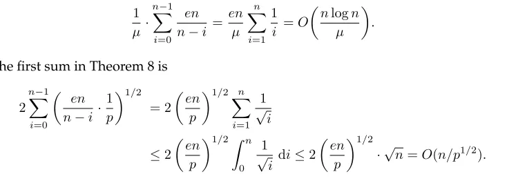
en n−i =

en µ n X i=1 1 i =O

nlogn µ

.

The first sum in Theorem 8 is

2 n−1

X

i=0

_en

n−i· 1 p

1/2

= 2

_en

p

1/2 n X i=1 1 √ i ≤2 _en p

1/2Z n

0

1

√

i di≤2

_en

p

1/2

For unimodal functions we choose a partitionA1, . . . , Ad+1whereAicontains all search

points with thei-th smallest function value. The probability of improving the fitness from leveliis at leastsi≥1/(en)because there is at least one search point in the next

fitness level which is at Hamming distance one. Theorem 8 gives an upper bound of

2 d X i=1 en p

1/2

+ d

X

i=1

en µ ≤2d·

en p

1/2

+den

µ =O

dn1/2

p1/2 +

dn µ

.

For Jump_kwe again chooseAito contain all search points with fitnessi, leading to sets A1, . . . , An and An+k. The levels A1, . . . , Ak−1 resemble those for OneMax (modulo

swapping the meaning of zeros and ones), and the same estimations for thesi apply.

The same holds for levelsAk, . . . , An−1, whereAicorresponds to a success probability

ofsi−kin the context of OneMax. So the expected time for getting to either of the two

best fitness levels, the setAn∪An+k, is bounded by twice the above upper bound for

OneMax. In case we have reachedAn, to reach the highest levelAn+k, a specific bit

string with Hamming distancekhas to be created. This has probability at least

sn≥

1 n k ·

1−_n1

n−k

≥ 1 n k ·

1−_n1

n−1

≥_en1k .

Theorem 8 and the above bound for OneMax give

O

_n

p1/2+

nlogn µ

+ 2

_enk

p

1/2

+en

k

µ =O

_nk/2

p1/2 +

nk µ

.

The speedups obtained are indeed significant, particularly for those functions where improvements are hard to find.

The proof of Theorem 9 uses well-known fitness-level partitions [8, 47], and hence it simply consists of plugging in known valuessi and simplifying. This shows how

easy it is to obtain results for parallel EAs based on analyses of panmictic EAs.

5

Parallel EAs with Two-Dimensional Grids and Tori

For two-dimensional grids and tori we adapt Theorem 4 in a similar manner, making an effort to get the best possible leading constant in the first term of the running time bound. We also consider applications of the resulting theorem similar to the applica-tions for ring graphs.

Theorem 10. Consider an island model running elitists EAs on a functionf with a fitness-level partitionA1 <f · · · <f Amand success probabilitiess1, . . . , sm−1. Let pbe (a lower

bound on) the probability that a specific island on fitness leveliinforms a specific neighbor in the topology in one generation. The expected parallel running time of the island model on a grid or torus topology whose side lengths are at leastõin both directions is bounded from above by

35/3

p2/3

m−1

X

i=1

1 s1i/3

+ 1

µ m−1

X

i=1

1 si

.

Proof. Note that within a square area of√k×√kvertices in the graph all shortest paths between any two vertices have at most2√k−2edges. So for every vertex in this area, the number of vertices that can be reached via up tok′_{:= 2}√_{k−2edges isn}′

k ≥k. We

pessimistically assumen′

k =k; if not, we consider a slower propagation process where

we remove edges of the graph to ensuren′

k =k. Applying Lemma 7 with respect to

the primed variablesk′:= 2√k−2,nk′ =kandc= 4we have that for everyk≤µthe

expected time untilkislands are informed is bounded from above by

max

(

16/3·√k−16/3

p ,

32/3·ln(4k)

p

)

.

We also get an upper bound ofk/(2p)using Johannsen’s variable drift theorem [21], Theorem 20 in the appendix, as before. If there is more than one uninformed vertex, there are always at least two vertices neighboring to informed ones. So the expected number of informed vertices increases by2pin expectation. Applying Johannsen’s drift theorem as for the bidirectional ring gives an upper bound ofk/(2p). It is easy to check that the best upper bound is as follows: for allk∈N

min

(

k

2p,max

(

16/3·√k−16/3

p ,

32/3·ln(4k)

p

))

≤6 √

k−1

p .

Now, if1 ≤ k := 3−2/3_·(p/s

i)2/3 ≤ µ(ignoring rounding issues) by Lemma 6 the

expected number of generations on fitness leveliis bounded from above by

6√k−1

p + 1 +

1 k·

1 si ≤

6·3−1/3

p2/3_s1/3

i

+ 3

2/3

p2/3_s1/3

i

= 3

5/3

p2/3_s1/3

i .

If3−2/3_·(p/s

i)2/3<1we trivially get an upper bound of

1 si ≤

32/3

p2/3_s1/3

i .

If3−2/3_·(p/s

i)2/3> µ, we get fork:=µan upper bound of

6√µ−1

p + 1 +

1 µ·

1 si

< 2·3

2/3

p2/3_s1/3

i +1 µ· 1 si .

Taking the maximum of the above upper bounds gives

max 3

5/3

p2/3_s1/3

i

, 2·3

2/3

p2/3_s1/3

i + 1 µ· 1 si ! ≤ 3

5/3

p2/3_s1/3

i

+1

µ· 1 si.

Summing over all fitness levels yields the claim.

The claim on the expected communication effort follows from Theorem 2.

Note that the communication effort in one generation is asymptotically as large as for ring graphs, but for large pthe upper bound on the parallel running time is generally smaller (or asymptotically equal, in case upper bounds are dominated by the term1/µ·Pm−1

i=1 1/si). Ifp < 3si then again the trivial upper bound1/si is better as

Compared to a single island, in a torus the expected waiting time for every fit-ness level can be replaced by its third root. This leads to improved upper bounds for unimodal functions and Jump_k.

Theorem 11. The following holds for the parallel (1+1) EA with transmission probabilitypon a grid or torus topology whose side lengths are at leastõin both directions:

• E(Tpar_{) =O} n p2/3 +

nlogn µ

forOneMax,

• E(Tpar) =Odn_p21//33 +

dn µ

for every unimodal function withd+ 1function values,

• E(Tpar_{) =O}n+nk/3

p2/3 +

nk µ

forJump_kwithk≥2.

Proof. We choose the same partitions as in the proof of Theorem 9. Note that the second terms in Theorem 8 and 10 are identical, so we only estimate the first terms and refer to Theorem 9 for the second terms.

For OneMax the first sum in Theorem 10 is

35/3

p2/3

n−1

X

i=0

en n−i

1/3

= 3

5/3_e1/3_n1/3

p2/3

n X i=1 1 i

1/3

≤ 3

5/3_e1/3_n1/3

p2/3

Z n

i=0

1 i

1/3

di

= 3

5/3_e1/3_n1/3

p2/3 ·

3

2 ·n

2/3₌38/3/2·e1/3n

p2/3 .

This gives an upper bound of

O

_n

p2/3 +

nlogn µ

.

For unimodal functions Theorem 10 gives

35/3

p2/3

d

X

i=1

(en)1/3+

d

X

i=1

en

µ ≤

35/3_d·e1/3_n1/3

p2/3 +

den

µ =O

_dn1/3

p2/3 +

dn µ

.

For Jump_kwe get

O

_n

p2/3 +

nlogn µ

+ 35/3·(en

k₎1/3

p2/3 +

enk

µ =O

_n+nk/3

p2/3 +

nk µ

.

6

Parallel EAs with Hypercube Graphs

Hypercube graphs are popular topologies in parallel computation. In ad-dimensional hypercube each vertex has a label ofdbits. Two vertices are neighboring if and only if their labels differ in exactly one bit. The number of vertices is then2d_{, and each vertex}

Theorem 12. Consider an island model running elitists EAs on a functionf with a fitness-level partitionA1 <f · · · <f Amand success probabilitiess1, . . . , sm−1. Let pbe (a lower

bound on) the probability that a specific island on fitness leveliinforms a specific neighbor in the topology in one generation. The expected parallel running time of the island model on a

(logµ)-dimensional hypercube graph withµislands is bounded from above by

25m+ 12Pm−1

i=1 log( 1

si)

p +

1 µ·

m−1

X

i=1

1 si .

The expected communication effort is by a factor of at mostpµlogµlarger than the expected parallel time.

Proof. In the notation of Lemma 7 we have for the hypercube and1 ≤ k ≤logµthat the number of vertices reachable with at mostkedges is bounded from below by

nk= k X i=1 µ i

≥2k.

As in the proof of Theorem 8 we considern′

k = 2k instead ofnk, justified by the fact

that we can remove edges in the graph to slow down propagation. Invoking Lemma 7 withk,n′

k= 2k, andc= 2, the expected time until2kvertices are informed is therefore

at most

16 ln(2·2k₎

p =

16·(ln 2)·(k+ 1)

p <

12(k+ 1)

p .

By Lemma 6 the expected time on fitness level i is hence bounded, for any integer

0≤k≤logµ, by

12(k+ 1)

p + 1 +

1

2k ·

1 si ≤

13

p +

12k

p +

1

2k ·

1 si

. (4)

Ifp/(12si) <1, we get a trivial upper bound of1/si ≤ 12/p. Ifp/(12si) > µ, which

impliesd <log(p/(12si))≤log(1/si), we get an upper bound of

13 + 12d

p +

1 µ·

1 si

< 13 + 12 log(

1

si)

p + 1 µ· 1 si .

Otherwise, (4) is minimized for2k_=p/(12s

i), leading to

13

p +

12 log(₁₂p_si)

p +

12

p ≤

25 p +

12 log(_s1_i)

p .

The maximum over all these bounds is at most

25 + 12 log(1

si)

p +

1 µ·

1 si.

Summing over all fitness levels yields the claim.

The claim on the expected communication effort follows from Theorem 2.

Theorem 13. The following holds for the parallel (1+1) EA with transmission probabilitypon a(logµ)-dimensional hypercube:

• E(Tpar_{) =O}n p +

nlogn µ

forOneMax,

• E(Tpar_{) =O}dlogn p +

dn µ

for every unimodal function withd+ 1function values,

• E(Tpar_{) =O}n+klogn

p +

nk µ

forJump_kwithk≥2.

Proof. For OneMax we have

n−1

X i=0 log ₁ si = n X i=1

logen

i = log n Y i=1 en i ! = log

_en_nn

n!

≤log

_en_nn

(n/e)n

= log e2n

= 2nlog (e).

Theorem 12 gives an upper bound of

25n+ 24nloge

p +O

_nlogn

µ

=O

_n

p + nlogn

µ

.

For unimodal functions Theorem 12 gives

25d+ 12dlog(en)

p +O

_dn

µ

=O

_dlogn

p +

dn µ

.

For Jump_kwe get, usinglog(enk_)≤log(ek_nk_{) =O(klogn),}

O

n p+

nlogn µ

+25 + 12 log(en

k₎

p +O

nk µ =O

n+klogn

p +

nk µ

.

If p = Ω(1), we get linear speedups for OneMax if µ = O(logn), and linear

speedups for unimodal functions where the boundO(dn)for a single island is tight, ifµ=O(n/logn). For Jump_k, ifk=O(n/logn)we can chooseµ =O(nk−1_{)to get a}

linear speedup. As can be seen from Table 1 the upper bounds on the expected parallel times for LO and Jump_k are much better for the hypercube than for rings and torus graphs, ifpis large.

7

Parallel EAs with Complete Topologies

Finally, we consider the densest topology, the complete graphKµ, where every island

is neighboring to every other island. The complete graph is interesting because it rep-resents an extreme case: the largest possible communication effort with regard to one generation, but also the fastest possible spread of information.

the fitness-level method. Hence our results for a parallel (1+1) EA with a complete topology andp= 1also apply to the (1+µ) EA. Forp <1the two models are generally different.

We start with a simple argument. Clearly, if there is at least one informed island, each other island will become informed with probability at leastp.

Theorem 14. Consider an island model running elitists EAs on a functionf with a fitness-level partitionA1 <f · · · <f Amand success probabilitiess1, . . . , sm−1. Let pbe (a lower

bound on) the probability that a specific island on fitness leveliinforms a specific neighbor in the topology in one generation. The expected parallel running time of the island model on a complete topology is

E(Tpar_{) ≤ m+}2m

p +

2 µ

m−1

X

i=1

1 si

.

The expected communication effort is by a factor of at mostpµ(µ−1) < pµ2 larger than the expected parallel time.

Proof. We estimate the expected time until at leastµ/2 islands are informed after an improvement. If more thanµ/2islands are uninformed, the expected number of islands that become informed in one generation is at leastpµ/2. By standard drift analysis arguments [16] the desired expectation is bounded from above by2/p.

By Lemma 6 we then get that the expected time on fitness leveliis at most

1 +2

p+ 2 µ·

1 si .

Adding these times for all fitness levels proves the claim.

The claim on the expected communication effort follows from Theorem 2.

As mentioned, the complete graph leads to a maximal spread of information. In comparison to the previous sections, we obtain the best upper bounds for the con-sidered function classes. However, a maximum amount of migration takes place in each generation, so the expected total communication effort is also highest (cf. Tables 1 and 3).

Theorem 15. Letµ ∈ N_{. The following holds for the expected parallel running time of the} parallel (1+1) EA with topologyKµ. In the casep= 1, the same holds for the (1+µ) EA:

• E(Tpar_{) =O}n p +

nlogn µ

forOneMax,

• E(Tpar_{) =O}d p +

dn µ

for every unimodal function withd+ 1function values, and

• E(Tpar_{) =O}n p +

nk µ

forJump_k withk≥2.

The proof is obvious by now.

The term2/pfor the time until at leastµ/2 islands are informed is a reasonable estimate ifpis large (e. g., p= Ω(1)). But for smallpthis estimation is quite loose as we have completely neglected thatallinformed vertices have a chance to inform other islands.

whether to migrate individuals to that island. Then this can be regarded as a complete topology with transmission probabilityp.

Values aroundp = 1/µseem particularly interesting as then in each generation one migration takes place for each island in expectation. In fact, we get different results forp >1/µandp <1/µ.

Lemma 16. Consider propagation with transmission probabilitypon the complete topology withµvertices. Letξ(k)be as in Lemma 6, then

ξ(µ)≤_min(pµ,8 log(µ)₁₎.

Proof. The claim is obvious for µ ≤ 2, so we assumeµ ≥ 3in the following. LetXt

denote the random number of informed vertices aftertiterations. We first estimate the expected time until at leastµ/2vertices become informed, and then estimate how long it takes to get fromµ/2informed vertices toµinformed ones.

IfXt=ieach presently uninformed vertex is being informed in one iteration with

probability (using Lemma 19 in the appendix)

1−(1−p)i_≥1− 1

1 +ip =

ip

1 +ip.

This holds independently from other presently uninformed vertices. In fact, the num-ber of newly informed vertices follows a binomial distribution with parametersµ−i

and ₁₊ip_ip. The median of this binomial distribution isi(µ−i)·1+pip (assuming that this

is an integer), hence with probability at least1/2we have at leasti(µ−i)·1+pip newly

informed vertices in one iteration. Hence, it takes an expected number of at most 2 iter-ations to increase the number of informed vertices byi(µ−i)·1+pip, which fori≤µ/2

is at leasti·2+pµpµ.

For every0 ≤ j ≤ log(µ)−2the following holds. Ifi ≥ 2j _{andi ≤ µ/2 then in}

an expected number of 2 generations at least2j·2+pµpµ new vertices are informed. The

expected number of iterations for informing a total of 2j new vertices is therefore at most2· 2+pµpµ. Then we have gone from at least2

j _{informed vertices to at least2}j+1

informed vertices. Summing up all times across allj, the expected time until at least

2log(µ)−1_{=µ/2vertices are informed is at most}

2(log(µ)−1)·2 +pµ

pµ .

Forpµ≤1we have2+_pµpµ ≤3/(pµ), yielding an upper time bound of6(log(µ)−1)/(pµ). Otherwise, we use 2+_pµpµ ≤3to get a bound of6(log(µ)−1).

nodes, usingh(i) := ₁₊₍i(µ_µ−₋i)_ip_)p as drift function, gives an upper bound of

1 + (µ−1)p

(µ−1)p +

Z µ/2

1

1 + (µ−i)p

i(µ−i)p di

≤ 1 + (µ_(µ −1)p

−1)p +

ln(µ−1)(1 +pµ)

pµ

≤ 1 +pµ

pµ +

1 µ(µ−1)p+

ln(µ−1)(1 +pµ)

pµ

≤ (ln(µ) + 1)(1 +pµ) +

1

µ−1

pµ .

Forpµ≤1this is at most

2 ln(µ) + 2 + 1

µ−1

pµ ≤

2 ln(µ) + 5/2

pµ .

Otherwise, this is at most

(ln(µ) + 1)·2pµ+_µpµ₋₁

pµ ≤2 ln(µ) + 5/2.

Together, along withln(µ)≤log(µ)this proves the claim.

Combining Lemma 16 with Lemma 6 gives the following. Apart from an additive termm, the case ofp≤1/µyields a bound where the first term is smaller by a factor of orderlog(µ)/µ. For fairly large transmission probabilities,p≥1/µ, in the first term we have replaced the factor1/pbylog(µ). These improvements reflect that the complete graph can spread information much more quickly than previously estimated in the proof of Theorem 14.

Theorem 17. Consider an island model running elitists EAs on a functionf with a fitness-level partitionA1 <f · · · <f Amand success probabilitiess1, . . . , sm−1. Let pbe (a lower

bound on) the probability that a specific island on fitness leveliinforms a specific neighbor in the topology in one generation. The expected parallel running time of the island model on a complete topology is bounded as follows. Ifp≥1/µwe have

E(Tpar) ≤ m+ 8mlogµ+ 1 µ

m−1

X

i=1

1 si

and ifp≤1/µwe have

E(Tpar) ≤ m+8mlogµ

pµ +

1 µ

m−1

X

i=1

1 si .

For our example applications, the refinements in Theorem 17 result in the follow-ing refined bounds. As we only get improved upper bounds forp=O(1/µ), we do not mention the special case of the (1+µ) EA withp= 1.