The Estimation of Place-to-Place Migration Flows Using an
Alternative Log-Linear Parameter Coding Scheme
James Raymer
Abstract
The log-linear model, with an alternative parameter coding scheme, is used in this paper to obtain estimates of place-to-place migration flows in situations where the data are inadequate or missing. The alternative parameter coding scheme is particularly useful in constructing the origin-destination interaction structure. To illustrate the method, two empirical examples are presented. The first demonstrates the effectiveness of the methodology by estimating known migration flows between states in the Western region of the United States during the 1985-1990 period. The second example focuses on estimating international migration flows in the Northern region of Europe during the 1999-2000 period where the data are incomplete. Both examples demonstrate the usefulness and generality of this particular method for estimating migration flows.
THE ESTIMATION OF PLACE-TO-PLACE MIGRATION FLOWS USING AN ALTERNATIVE LOG-LINEAR PARAMETER CODING SCHEME
James Raymer
July 30, 2004
Contact Information:
Mailing Address: Division of Social Statistics School of Social Sciences University of Southampton Highfield Southampton S017 1BJ
United Kingdom Telephone: +44 23 8059 2935
Email: [email protected]
ABSTRACT
The log-linear model, with an alternative parameter coding scheme, is used in this paper to obtain estimates of place-to-place migration flows in situations where the data are inadequate or missing. The alternative parameter coding scheme is particularly useful in constructing the origin-destination interaction structure. To illustrate the method, two empirical examples are presented. The first demonstrates the effectiveness of the
methodology by estimating known migration flows between states in the Western region of the United States during the 1985-1990 period. The second example focuses on estimating international migration flows in the Northern region of Europe during the 1999-2000 period where the data are incomplete. Both examples demonstrate the usefulness and generality of this particular method for estimating migration flows.
THE ESTIMATION OF PLACE-TO-PLACE MIGRATION FLOWS USING AN ALTERNATIVE LOG-LINEAR PARAMETER CODING SCHEME
1. INTRODUCTION
Estimates of place-to-place migration flows provide national and regional governments with the means to improve their planning policies directed at supplying
particular social services or at continuing, increasing, or decreasing levels of interregional or international migration. Furthermore, our understanding of how or why populations change requires relatively accurate estimates of migration flows. Without these, the ability to predict or attempt to control that change is limited. The purpose of this paper is to illustrate a
methodology for obtaining estimates of place-to-place migration flows for a variety of data situations. This work follows some recent developments on the identification and description of migration spatial structures in terms of categorical log-linear and logit model parameters (Rogers et al. 2002; Rogers, Willekens and Raymer 2001, 2002, 2003). In particular, this research provides an alternative parameter interpretation of the log-linear model, which is useful for guiding the modeling of the interactions between origins and destinations of migration flows --- the key element required for more accurate predictions.
Models for estimating migration flows are necessary because the data are often inadequate or missing (Willekens, 1999). For example, the sample size of the survey used to obtain the migration statistics may have been too small for the level of detail in the analysis. This tends to cause unexpected irregularities in the data. The level of demographic,
socioeconomic, or spatial detail required for a particular study may not have been collected. The survey question about migration might not fit the research question regarding migration.
There may be situations in which the required migration data are available but cannot be considered reliable, such as emigration data provided by sending countries. And, there may be significant non-responses in the survey. Aside from collecting the missing data, the solutions to the above problems include using ancillary data, smoothing the data, or estimating the missing data.
For the estimation of migration flows, gravity and spatial interaction models are the most commonly applied because they are still considered to be the best models for accurately predicting aggregate-level migration flows (Fotheringham, Brunsdon and Charlton
2000:217). This is true despite the known behavioral inadequacies of these models (see, e.g., Sheppard 1979). The gravity model is a relatively simple model which includes the factors of population sizes of the origin and destination regions, the distance between them, and some measure of competition or attractiveness (Lowry 1966:7). The spatial interaction model is essentially a statistical form of the gravity model. Wilson’s (1971) introduction of “families of spatial interaction models” using entropy-maximization techniques was a key turning point in the modeling of spatial patterns of migration. Soon after, this framework was applied for use in modeling migration flows (i.e., Plane 1981; Willekens 1977, 1980; Willekens, Por and Raquillet 1981).
Willekens (1983) demonstrated that the log-linear model could be used to model spatial interaction patterns. In general, log-linear models are used to model contingency tables. A migration flow table can be considered a two-way (i.e., origin by destination) contingency table, where the cells represent counts of migrants. The advantage of the log-linear model over the general spatial interaction model is that it has a well-formed theory and methods, associated in the framework of contingency-table analysis or discrete multivariate
analysis (Willekens 1999). In addition to log-linear models of migration estimation, similar work has been carried out in the name of Poisson regression (Flowerdew 1991; Flowerdew and Aitkin 1982; Flowerdew and Lovett 1988).
Iterative proportional fitting (Deming and Stephan 1940) is another technique that has been used to obtain, or update tables of, place-to-place migration flows (e.g., Nair 1985; Rees and Duke-Williams 1997; Willekens 1982; Willekens, Por and Raquillet 1981). More
recently, Schoen and Jonsson (2003) introduced an alternative form of the iterative fitting procedure, termed Relative State Attraction, to estimate multistate transition rates. This technique assumes that the marginal totals of a migration flow table are available. The flows are estimated by adjusting, through iteration, a corresponding table of numbers, for instance, a historical set of place-to-place migration flows, to fit the given marginal totals of the table. Note, for a two-way contingency table, the iterative proportional fitting procedure produces the same results as a log-linear main effects model with an offset.
In the next section, a place-to-place migration flows situation containing inadequate and missing data is set out, namely international migration flows between countries in Northern Europe during the 1999-2000 time period. This is followed by a presentation of a general methodology for estimating missing or inadequate migration flow data. Then, two empirical demonstrations are put forward. The first, in Section 4, illustrates the effectiveness of the methodology by modeling known migration flows between states in the Western region of the United States during the 1985-1990 period. The second example, in Section 5, applies the methodology to estimate the unknown or inadequate European migration data mentioned above. The purpose of both examples is to show that a single methodology can be used to estimate both internal and international migration flows.
2. THE PROBLEM: INADEQUATE AND MISSING INTERNATIONAL MIGRATION FLOW DATA IN THE NORTHERN REGION OF EUROPE Because of differences in data availability, quality, and measurement, no consistent set of migration flow estimates exist between the countries in Europe. At best, net migration and some general directions of the migration patterns are known. The countries in the Western and Northern regions of Europe tend to have better (or excellent) migration statistics, whereas in the Eastern and Southern regions, much of the patterns are largely unknown. As such, reports on the patterns of migration in Europe have largely relied on known patterns (e.g., de Beer and van Wissen 1999; Eurostat 1999; Massey et al. 1998; Salt 1996, 2001). This paper begins to address the problem of missing and inconsistent migration flow data in Europe by focusing on the international migration patterns between countries in the Northern region of Europe during the 1999-2000 period. For most of these countries, international migration is the most important factor of demographic change. In fact, several now have proportions of foreign populations similar to the “traditional” immigration countries of the United States, Australia, and Canada (Massey et al. 1998).
The European migration data set out in this article comes from the Eurostat
NewCronos database (as of February 2003). Eurostat is considered Europe’s main statistical agency responsible for collecting and storing macroeconomic and social statistical data. For international migration patterns in Europe, there are two major agencies that provide an international database of migration statistics (King 2002:101; Salt 2001): Eurostat and the Organization for Economic Co-Operation and Development (OECD). Both agencies have large databases (i.e., NewCronos and SOPEMI, respectively) and produce annual reports of international migration flows (e.g., Eurostat 2000; SOPEMI 2003). The data gathered by
these two agencies are similar to each other in that they obtain their migration data by sending out questionnaires to the statistical agencies in each of the countries representing Europe and elsewhere (for the case of OECD). The statistical agencies then report back their observed or estimated numbers of migrants for certain specified time periods. Neither Eurostat or OECD alters these data --- they simply report them as given. As the numbers come from various statistical agencies with varying methods of data collection and definitions, some inconsistencies naturally result.
One set of international migration flows, obtained from the available immigration
flow data provided by Eurostat, are set out in Table 1. Here, we see that Denmark, Finland, Iceland, Norway, and Sweden provide origin-destination-specific data. Ireland and the United Kingdom provide some detailed information, but not for all origins and destinations. Estonia, Latvia, and Lithuania provide no immigration data at all. In total, we have information on 51 out of a possible 90 country-to-country flows (or 57 percent of the information available). Similarly, an additional migration flow table can be produced from the available emigration
data, also provided by Eurostat. These flows are set out in Table 2.
For comparison purposes, consider the migration flows between Scandinavian countries (i.e., Denmark, Iceland, Norway, and Sweden) in Tables 1 and 2. These numbers are relatively similar to each other. For example, according to the immigration flow table (i.e., Table 1), there were 3,188 migrants from Denmark to Norway. This number is much like the one found in the emigration flow table (i.e., 3,141; see Table 2). Next, consider the Norway to United Kingdom migration flow. In this case, two very different numbers arise in Tables 1 and 2. In Table 1, there are 3,188 persons who migrated from Norway to the United Kingdom, whereas in Table 2, there are 1,735 persons. The former number comes from the
United Kingdom government. The latter comes from the Norwegian government. This is just one example of inconsistency. There are many more to be found between the two tables. Much of this inconsistency is likely due to different data collection systems (e.g., survey-based versus registration-survey-based) and to the timing of the collection (Poulain 1994).
Table 1. International migration flows based on available immigration data for the Northern region of Europe, 1999-2000
Country of Destination Country
of Origin Den. Est. Fin. Ice. Ire. Lat. Lith. Nor. Swed. U.K. Total
Denmark 355 1,446 2,734 2,194 2,025
Estonia 257 784 6 85 262
Finland 448 46 1,380 3,647 1,556
Iceland 1,267 54 463 384
Ireland 266 41 6 73 199
Latvia 376 44 7 116 169
Lithuania 499 21 33 104 111 149
Norway 3,188 955 602 5,496 3,814
Sweden 2,298 3,229 572 6,044 1,539
U.K. 3,965 586 167 21,611 2,014 2,447
Total 12,564 6,069 2,885 13,013 14,909
Non-Migrants Not Available
Table 2. International migration flows based on available emigration data for the Northern region of Europe, 1999-2000
Country of Destination Country
of Origin Den. Est. Fin. Ice. Ire. Lat. Lith. Nor. Swed. U.K. Total
Denmark 232 392 1,422 368 322 325 2,786 2,295 4,291 12,433
Estonia
Finland 415 264 43 101 22 10 1,383 3,695 941 6,874
Iceland 1,327 3 60 15 0 5 492 406 201 2,509
Ireland 10,188
Latvia
Lithuania
Norway 3,141 40 978 606 77 59 40 5,523 1,735 12,199
Sweden 2,196 71 3,178 548 251 33 19 5,912 3,281 15,489
U.K. 1,831 4,849 220 2,164 4,352
Total
Non-Migrants Not Available
Despite the known inconsistencies, the immigration flow (Table 1) and emigration flow (Table 2) data are combined in Table 3 with the assumption that some data is better than no data. By combining both tables of flows, 74 of the 90 flows are now (in some way)
accounted for. Now, the only missing data are the migration flows between Estonia, Ireland, Latvia, Lithuania, and the United Kingdom. Preference for the numbers in Table 3 was given to the immigration data. Numbers from the emigration table (Table 2) were used only when numbers from the immigration table (Table 1) were not available. The immigration data are generally considered more reliable because immigrants are present in the country providing the data. Emigration data, on the other hand, is based on either respondents reporting back to their country of origin, or from statements on intended destinations. In the latter case, it is not possible to verify whether or not these migrants actually migrated to where they said they would. However, in some cases it could be argued that the emigration data from countries
with strong registration systems might be more accurate than immigration data based from either weak registration systems or surveys (Poulain 1999).
Table 3. International migration flows based on available immigration and emigration data for the Northern region of Europe, 1999-2000*
Country of Destination Country
of Origin Den. Est. Fin. Ice. Ire. Lat. Lith. Nor. Swed. U.K. Total
Denmark 232 355 1,446 368 322 325 2,734 2,194 2,025 10,001
Estonia 257 784 6 85 262
Finland 448 264 46 101 22 10 1,380 3,647 1,556 7,474
Iceland 1,267 3 54 15 0 5 463 384 201 2,392
Ireland 266 41 6 73 199
Latvia 376 44 7 116 169
Lithuania 499 21 33 104 111 149
Norway 3,188 40 955 602 77 59 40 5,496 3,814 14,271
Sweden 2,298 71 3,229 572 251 33 19 6,044 1,539 14,056
U.K. 3,965 586 167 21,611 220 2,014 2,447
Total 12,564 6,069 2,885 13,013 14,909
Non-Migrants Not Available
* Preference given to immigration data.
Finally, the numbers in the above table are considered in this paper to be the best available information for international migration between countries in Northern Europe during the 1999-2000 period. This information is used later in this paper to obtain a complete and consistent set of estimated migration flows between the ten countries in Northern Europe. But first, in the next section, a proposed model solution is presented for obtaining these numbers.
3. A PROPOSED MODEL SOLUTION
This section consists of two parts. In Section 3.1, the log-linear model, with an alternative parameter coding scheme, is put forward for the purpose of obtaining estimates of place-to-place migration flows in situations where the data are inadequate or missing. The alternative parameter coding scheme is particularly useful in constructing the origin-destination interaction structure, which is then incorporated into the “offset” (discussed below). In Section 3.2, the model is tested on known internal migration flows between states in the United States West region.
3.1 Modeling the Spatial Patterns of Migration
The modeling framework described in this paper focuses on one stage in the modeling process of migration. There are three distinct stages of modeling aggregate levels of
migration (Raymer 2003). The first stage focuses on estimating the gross flows of migration (i.e., in-migration and out-migration or immigration and emigration) using ordinary least squares regression (e.g., Cadwallader 1992). These estimates form the marginal totals of a migration flow table. The second stage, which is the topic of this paper, focuses on estimating the spatial patterns using spatial interaction or log-linear models (e.g., Willekens 1983). The third stage focuses on estimating the age patterns using, for example, multiexponential model migration schedules (Rogers and Castro 1981). The three stages are hierarchical and, ideally, should be constrained so that the estimates are consistent with the net migration obtained via the demographic accounting model (e.g., Siegel and Hamilton 1952). This paper assumes that the gross flows of in-migration and out-migration (i.e., the marginal totals of a migration flow table) are known or have already been estimated.
The models set out in this paper estimate the migration flows between origins i and destinations j. The counts of origin-destination-specific migrants are denoted . When i = j, the persons are said to be “stayers”. Stayers are non-migrants or persons who may have migrated out and back within the time interval. The numbers of persons living in a particular place at the beginning of the time interval are denoted by n
ij
n
i+. The numbers of persons living
in a particular place at the end of the time interval are denoted n+j.
3.1.1 Describing the Spatial Patterns of Migration
Place-to-place migration flows are often set out in two-way (i.e., origin by
destination) contingency tables. These migration flow tables can be disaggregated into four separate components (Rogers et al. 2002): an overall component representing the level of migration, an origin component representing the relative “pushes” from each region, a
destination component representing the relative “pulls” to each region, and an
origin-destination interaction component representing the physical or social distance between places not explained by the other three components. The motivation for this paper comes from this approach to examining migration flows.
A model that is very useful for describing the spatial patterns of migration is the log-linear model. This model, in multiplicative form, is specified as:
OD ij D j O i ij
nˆ =ττ τ τ (1)
where is the predicted migration flow in cell ij. The parameters of the model ( s) have superscripts O and D denoting origin i and destination j, respectively. The overall effect is
ij
nˆ τ
denoted by ϑ, the origin main effect is denoted by , the destination main effect is denoted by , and the origin-destination interaction effect is denoted by . The log-linear model typically assumes a Poisson probability distribution because its properties are relatively simple and well known and, like counts, the outcomes can only be positive. Note, another distribution that is often used to model counts is the negative binomial regression model. Unlike the Poisson regression model, this model allows the variance to exceed the conditional mean. The parameters of this model are estimated using maximum likelihood methods. Finally, log-linear models and Poisson regression models are analogous when the data are categorical.
O i τ
D j
τ OD
ij τ
Because different statistical packages use different reference coding schemes, it is important to know how the parameters are interpreted for purposes of analysis and
estimation. The coding scheme should be based on the research question. The parameters of the log-linear model in its multiplicative form are interpreted as odds and odds ratios with reference to some category. The two most popular reference category coding schemes are the cornered-effect coding scheme and the geometric mean coding (effect coding) scheme. A third coding scheme is presented that is not in the literature but is believed by the author of this paper to be more intuitive and practical. This coding scheme is called the total sum reference coding scheme. Cornered-effect coding implies that the parameters are interpreted with reference to a single cell in the table. Most standard statistical software packages use this coding scheme as the default. For example, SPSS uses a last reference category coding
scheme, whereas Stata uses a first reference category coding scheme. Geometric mean coding implies that the parameters are interpreted with reference to the overall geometric mean of
values in the table. Finally, the total sum reference coding scheme implies that the parameters are interpreted with reference to the overall total migration level (i.e., ) associated with the migration flow table.
+ +
n
When cornered-effect coding (e.g., the last reference category) is used, the main effects correspond to the reference category (cell) only. This scheme is not as intuitive for the analysis of migration flows because often researchers are interested in overall patterns, not patterns related to a specific region. Also, for both the first category and last category coding schemes, migrants are compared to non-migrants. This causes parameter interpretation to be particularly confusing.
The effects of the geometric mean coding model are expressed in terms of ratios between geometric means. Note, for a detailed description, refer to Willekens (1983). For this coding scheme, any increase or decrease to any one cell value (e.g., in the diagonal) would alter all the parameter values, because the relative differences between the cells would change. The main effects and interaction effects would stay the same only if one divided all the cells by the same number (i.e., by 1000, by 2000, by 1000000, etc.). In that case, only the overall effect would change. The advantage to this parameter coding scheme is interpretation. One is basically comparing odds and odds ratios of averages.
For the model that uses the total sum reference category coding scheme, the overall
main effect is equal to τ=
∑
, the main effects are equal to ij ij n ⎥ ⎦ ⎤ ⎢ ⎣ ⎡ τ = τ∑
j ij O i n 1 and ⎥ ⎦ ⎤ ⎢ ⎣ ⎡ τ = τ∑
i ij D j n 1, and the interaction effects are equal to . The constraints of
the model are and
D j O i ij OD
ij =n /ττ τ τ 1 j D j i O
i = τ =
τ
∑
∑
1 i OD ij D j j OD ij Oi τ =τ τ =
τ
∑
∑
. The overall effect is simplythe overall level of the migration flow table. The origin effect is the proportion of all out-migrants from origin i. Likewise, the destination effect is the proportion of all in-out-migrants to destination j. Multiply these three effects together, and one gets an expected migration flow which uses information obtained from the marginal totals, not the cell values. Finally, the interaction effect essentially measures the strength of connection between two places (i.e., observed divided by expected flows).
The total reference category coding scheme has some clear advantages over the other coding schemes. This coding scheme relies entirely on the marginal totals, which is important since one is more likely to have the marginal totals than the origin-destination-specific flows. Also, the interaction effect parameters are simpler to interpret. They represent the ratio of observed migration flows to expected migration flows, where the latter is obtained by multiplying an overall level, a proportion observed in the row-sum marginal total, and a proportion observed in the column-sum marginal total. This method of coding is very useful for explaining migration flow tables and also for estimating a set of interaction effects when the data are incomplete, as is demonstrated later on in this paper. The main disadvantage of the total sum reference category coding scheme is that it is not an option in standard
statistical packages, so one is forced to translate between different coding schemes. However, the results produced from the total reference category coding scheme are the same as the results produced by either geometric mean or cornered-effect coding schemes; the difference lies in the interpretation of the parameters and in finding a logical way to estimate migration flows based on limited information.
3.1.2 Models for Imposing Spatial Structures of Migration
If the data are incomplete, auxiliary information may be used to predict migration flows (see, for example, Rogers, Willekens and Raymer 2003). Let denote a hypothetical migration flow table. The migration flow table for the current period may be predicted on the basis of, for example, information regarding the aggregate number of migrants living in regions i and j at the beginning and end of the time interval, n
* ij n
i+ and n+j, respectively, and
some information on the interaction between places represented by n*ij. The model then is:
D j O i * ij ij n
nˆ = ττ τ . (2)
The result of the above model is a migration flow table that exhibits the level of a current period, but adopts the structure of the offset, n*ij.
Contingency table analysis of migration flow data is generally difficult because of the fact that most people stay in their region of residence during the interval being studied. This results in much larger values in the diagonal elements than in the off-diagonal elements of a two-way contingency table. Because the diagonal values are so much larger, they tend to dominate the analysis and estimation process. To deal with this imbalance, one must either control for the diagonal elements, e.g., with structural zeros, or use models that separate the diagonal effects from the off-diagonal effects, e.g., with generation and distribution
components (Rogers, Willekens and Raymer 2001). The modeling strategy in this paper adopts the former --- structural zeros and the method of offsets --- because it is more
straightforward. Note, a main effects log-linear model without an offset predicts the non-migrants (i.e., diagonal values).
The iterative proportional fitting procedure produces the same results as those produced by the log-linear model with an offset. In this case, the marginal totals are given (the nij’s are assumed to be unavailable) and the offset includes ones in the off-diagonals and
zeros in the diagonal. The iterative procedure works by adjusting the offset to fit the marginal totals of the observed table. First, the values in the offset are proportionally forced to fit the row sums and, in the next iteration, they are proportionally forced to fit the column sums. By including zeros in the offset, the predicted values for those cells are ensured to equal zero in each of the iterations. The iteration process continues until the predicted migration data satisfy both the row and column marginal totals.
Finally, the observed data are perfectly predicted if one applies an offset that is obtained by dividing the observed values by the corresponding set of predicted values obtained using a main effects model with an offset that includes zeros in the diagonals and ones in the off-diagonals (as described above). Knowing this is a very important start because, with the total sum reference category coding scheme, we now have a simple platform to apply any available information, qualitative or quantitative, to improve our estimates provided that the marginal total information is available.
3.2 Testing the Model Solution: Estimating Interstate Migration in the U.S. West
The observed internal migration flow patterns between states in the West region of the United States during 1985 to 1990 are estimated in this subsection. For this illustration, the answers are known. The migration data come from a special 1990 census tabulation that represented the full sample of the long form respondents (U.S. Census Bureau 1993). Table 4
16
contains the observed migration flows between the thirteen states in the West region and the “Rest of U.S.”. The numbers of non-migrants, persons who out-migrated and returned within the time interval, and those who immigrated or emigrated are excluded. In total, there were 7.6 million migrants between these regions with California and Rest of the U.S. being the dominant regions (i.e., 61 percent of all out migration came from these regions and 56 percent of all migrants went to these two regions). Aside from the flows entering and leaving the two bigger regions, there were relatively large flows (over 20,000) from Colorado and New Mexico to Arizona, Arizona to Nevada, Washington to Oregon, and Alaska, Colorado, Idaho, Montana, and Oregon to Washington.
3.2.1 Analyzing the Observed to Expected Ratios of Migration Flows
Table 4. Interstate migration in the U.S. West, 1985-1990
State of State of Residence, 1990
Residence, Rest
1985 AK AZ CA CO HI ID MT NV NM OR UT WA WY of U.S. Total
AK
5,273 23,124 4,000 3,977 3,856 1,661 2,687 1,402 14,034 1,880 30,180 532 61,484 154,090 AZ 2,753 109,134 19,962 3,988 4,832 2,680 20,645 15,003 11,466 12,297 18,421 1,671 210,792 433,644 CA 11,493 136,465 62,397 44,862 26,887 11,990 110,985 27,437 128,797 38,356 155,394 5,114 1,041,070 1,801,247 CO 4,219 38,514 99,461 5,105 5,584 4,765 14,751 15,207 11,093 11,932 20,715 8,492 303,874 543,712 HI 1,990 4,720 54,098 4,868 1,028 541 3,994 1,314 5,210 1,737 11,885 198 95,626 187,209 ID 2,490 7,561 24,342 4,400 1,220 4,581 8,403 1,769 17,133 18,455 31,111 2,160 33,496 157,121 MT 2,434 7,448 16,442 6,471 1,057 7,265 5,423 1,666 8,350 3,491 24,817 6,044 46,219 137,127 NV 1,030 10,934 51,894 4,261 1,534 4,215 1,295 1,972 7,762 6,744 7,337 869 54,220 154,067 NM 1,451 23,080 29,828 15,604 1,191 1,259 1,200 7,050 3,068 3,718 5,885 1,037 109,847 204,218 OR 6,830 11,268 80,550 6,145 3,910 11,925 3,353 8,223 1,648 5,298 78,006 1,057 62,662 280,875 UT 1,450 18,018 51,265 12,398 2,252 11,837 2,635 16,874 3,501 7,387 13,508 4,349 67,759 213,233 WA 12,003 17,255 99,980 10,611 8,538 19,696 7,876 7,560 2,989 59,020 7,685 1,547 155,126 409,886 WY 1,110 8,092 12,762 14,482 520 3,741 5,674 6,744 2,724 3,606 7,678 5,438 46,408 118,979 Rest U.S. 56,352 361,193 1,321,953 300,115 88,799 35,417 36,272 113,580 116,129 86,521 57,800 223,459 29,216 2,826,806 Total 105,605 649,821 1,974,833 465,714 166,953 137,542 84,523 326,919 192,761 363,447 177,071 626,156 62,286 2,288,583 7,622,214
18
[image:21.612.87.633.128.338.2]est
Table 5. Ratios of observed to expected interstate migration flows in the U.S. West, 1985-1990
Destination
R
Origin AK AZ CA CO HI ID MT NV NM OR UT WA WY of U.S.
AK 0.000 0.515 0.598 0.539 1.554 1.834 1.289 0.538 0.473 2.493 0.691 3.067 0.561 0.950
AZ 0.572 0.000 0.946 0.903 0.523 0.771 0.697 1.386 1.700 0.683 1.515 0.628 0.591 1.093
CA 0.463 0.866 0.000 0.546 1.138 0.831 0.604 1.443 0.602 1.486 0.915 1.026 0.350 1.045
CO 0.713 1.026 0.701 0.000 0.544 0.724 1.008 0.805 1.401 0.537 1.195 0.574 2.442 1.281
HI 1.009 0.377 1.144 0.537 0.000 0.400 0.343 0.654 0.363 0.757 0.522 0.988 0.171 1.209
ID 1.508 0.722 0.615 0.580 0.466 0.000 3.473 1.644 0.584 2.976 6.627 3.090 2.227 0.506
MT 1.699 0.819 0.479 0.982 0.465 3.891 0.000 1.222 0.633 1.670 1.444 2.840 7.178 0.805
NV 0.624 1.044 1.312 0.562 0.586 1.960 0.983 0.000 0.651 1.349 2.423 0.729 0.896 0.820
NM 0.672 1.686 0.577 1.573 0.348 0.448 0.696 1.055 0.000 0.408 1.021 0.447 0.818 1.270
OR 2.262 0.588 1.112 0.443 0.816 3.030 1.390 0.879 0.297 0.000 1.040 4.235 0.595 0.518
UT 0.645 1.262 0.951 1.199 0.631 4.039 1.466 2.422 0.848 0.941 0.000 0.985 3.290 0.751
WA 2.647 0.600 0.920 0.509 1.187 3.333 2.174 0.538 0.359 3.731 1.005 0.000 0.580 0.853
WY 0.894 1.028 0.429 2.539 0.264 2.314 5.726 1.755 1.197 0.833 3.668 0.719 0.000 0.933
Consider, for example, the California to Arizona observed to expected ratio of 0.866. This value states, controlling for the relative shares of in-migration and out-migration and zeros for non-migrants, that the observed flow is 87 percent of the expected flow. This ratio can then be compared, for example, to the Idaho to Utah migration flow, which has a ratio of 6.627. In this case, the observed flow of 18,455 is almost seven times greater than the
expected flow of 2,785. The expected flow between these two states was small because both Idaho and Utah sent and received relatively few migrants in comparison to other states. As another example, consider the value of 0.546 for the ratio corresponding to the California to Colorado migration flow. This ratio tells us that the observed flow of 62,397 migrants was a little more than half the expected flow of 114,280 migrants.
Two overall patterns are found in the ratios of observed to expected migration flows set out in Table 5. The first is that proximity to other states is important. For example, Idaho exhibits ratios with values much greater than one with its neighboring states of Montana, Nevada, Oregon, Utah and Wyoming. This is true for both Idaho’s in-migration and out-migration. The exception is the interactions with California, which were less than one. The second general pattern found is that states with smaller population sizes tend to have more variation in their ratios than states with larger populations. For example, consider the ratios for migration flows associated with Wyoming, which range from 0.171 (Hawaii to Wyoming) to 7.178 (Montana to Wyoming), whereas for the Rest of U.S., the range was 0.495 (Rest of U.S. to Oregon) to 1.302 (Rest of U.S. to Colorado).
The expected values used in the denominator to calculate the ratios set out in Table 5 are necessary when one wants to control for the diagonal in the modeling of migration flows. For estimation purposes, this represents the baseline and the key to including hypothetical
relationships or partial information. When all of the observed to expected ratios are used as an offset in a log-linear main effects model, the observed values are perfectly predicted. When no interaction information is known, one is forced to use zeros in the diagonal and ones in the off-diagonals. In between these two situations (i.e., all information and no information) are a multitude of options.
3.2.2 Missing Data Scenarios
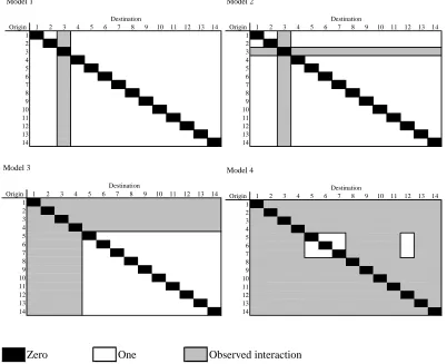
The diagrams set out in Figure 1 represent four partial data scenarios of interstate migration in the West. The data scenario presented in Model 1 includes California’s observed in-migration flows. Model 2 includes both in-migration and out-migration flows for
California. Model 3 includes in-migration and out-migration flows for the states of Alaska, Arizona, California, and Colorado. And Model 4 includes in-migration and out-migration for all states, except Hawaii, Idaho, Montana, and Washington. For each of these scenarios, an offset was constructed that included zeros in the diagonal, the observed to expected ratios for the available data, and ones for all other interactions.
Origin 1 2 3 4 5 6 7 8 9 10 11 12 13 14 1 2 3 4 5 6 7 8 9 10 11 12 13 14 Destination Model 1
Origin 1 2 3 4 5 6 7 8 9 10 11 12 13 14 1 2 3 4 5 6 7 8 9 10 11 12 13 14 Destination Model 2
Origin 1 2 3 4 5 6 7 8 9 10 11 12 13 14 1 2 3 4 5 6 7 8 9 10 11 12 13 14 Model 3 Destination
[image:24.612.79.481.84.411.2]Origin 1 2 3 4 5 6 7 8 9 10 11 12 13 14 1 2 3 4 5 6 7 8 9 10 11 12 13 14 Model 4 Destination Observed interaction One Zero
Figure 1. Four partial data scenarios of interstate migration in the West (1=AK, 2=AZ, 3=CA, 4=CO, 5=HI=, 6=ID, 7=MT, 8=NV, 9=NM, 10=OR, 11=UT, 12=WA, 13=WY, and 14=Rest of U.S.)
A contiguity offset was also constructed to represent neighboring states in the West. (Note, AK’s neighbours are HI, ID, MT, OR, and WA and HI’s neighbours are AK, CA, OR, and WA.) When the values in the contiguity matrix were regressed against the ratios of observed to expected migration flows (see Table 5), a significant relationship was found with an R2 of 0.264. The bivariate regression equation expressing this relationship was:
1 i) 0.065 0.432X Y
ln( =− +
where Yi represented the ratio of observed to expected migration and X1 the contiguity
matrix. When two states were neighbors (i.e., X1 = 1), the ratio was predicted to be 1.443.
When two states were not neighbors (i.e., X1 = 0), the predicted ratio was 0.937. This
information can be included along with available information to better estimate the missing data. Of course, in a missing data situation, the above ratios would not be known. To make the scenarios more realistic, four regressions were run based on the amount of information available. For Model 1, the predicted ratio for neighbors was 1.080 and 1.010 for neighbors. For Model 2, the predicted ratio for neighbors was 1.153 and 0.996 for neighbors. For Model 3, the predicted ratio for neighbors was 1.289 and 0.988 for neighbors. And, for Model 4, the predicted ratio for neighbors was 1.415 and 0.931 for non-neighbors. These predicted ratios, along with the available observed ratios, were included in an offset to estimate the missing data for the four model scenarios (Figure 1).
The offsets created from the four available data scenarios and from the contiguity matrix were used to predict the observed migration flows in the West region. The coefficient of determination ( =
∑
(
−)
∑
(
ij−)
22 ij 2 n n / n nˆ
R ), chi-square (
(
)
ij2 ij ij 2 nˆ / nˆ n
∑
− =χ ), and
likelihood-ratio (G2 =2
∑
nijlog(
nij/nˆij)
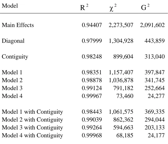
) goodness-of-fit indicators of these predictions are set out in Table 6 below. As expected, the results improved as more information was added. The predictions started out with a log-linear main effects model. This model produced a of 2,273,507. The model fit improved substantially to 1,304,928 when structural zeros in the diagonal were included using an offset. When the offset also included contiguity (i.e., 1.443 for neighbors and 0.937 for non-neighbors), the statistic dropped to 899,604. For the four available data scenarios, the statistics dropped from 1,157,407 (Model 1) to 73,460(Model 4). When contiguity was included with the four available data scenarios, the statistic dropped from 1,061,575 (Model 1 with contiguity) to 68,185 (Model 4 with contiguity).
[image:26.612.82.354.233.466.2]2 χ
Table 6. Comparison of different log-linear models used to predict interstate migration flows in the U.S. West, 1985-1990
Model 2
R χ2 G2
Main Effects 0.94407 2,273,507 2,091,602
Diagonal 0.97999 1,304,928 443,859
Contiguity 0.98248 899,604 313,040
Model 1 0.98351 1,157,407 397,847
Model 2 0.98878 1,036,878 341,745
Model 3 0.99124 791,182 252,664
Model 4 0.99967 73,460 24,277
Model 1 with Contiguity 0.98443 1,061,575 369,335 Model 2 with Contiguity 0.99039 862,362 294,044 Model 3 with Contiguity 0.99264 594,663 203,133 Model 4 with Contiguity 0.99968 68,185 24,177
The goodness-of-fit values set out in Table 6 show how the overall model fits improve with added information. To examine some particular origin-destination-specific migration flows, consider the comparison of five model scenarios the set out in Figure 2, which includes just the in-migration patterns to Idaho --- a state in which no observed migration data were included in any of the scenarios. Model 0 assumes no available information and includes an offset with zeros in the diagonal and ones in the off-diagonals. Models 1, 2, 3, and 4 corresponds to the four scenarios set out in Figure 1, where the available observed to expected ratios are included along with the predicted ratios based on contiguity. In Figure 2,
there are some interesting patterns. First, for flows from Hawaii, Montana, and Washington, none of the models performed that well. For the other ten states, the predicted values were very close to the observed values by Model 4.
0 10 20 30 40 50 60 70
AK AZ CA CO HI MT NV MT OR UT WA WY R.U.S.
Th
o
u
sa
n
d
s
[image:27.612.101.499.201.452.2]Model 0 Model 1 Model 2 Model 3 Model 4 Observed
Figure 2. Comparison of predicted and observed migration flows to Idaho: Model 0 (no data available), Model 1 (California in-migration data available), Model 2 (California in- and migration available), Model 3 (Alaska, Arizona, California, and Colorado in- and
out-migration data available), and Model 5 (all data available, except Hawaii, Idaho, Montana, and Washington in- and out-migration).
To summarize, the origin-destination-specific migration flows between states in the U.S. West region were modeled effectively using a log-linear main effects model with an offset. The key to the modeling strategy involved creating a good offset. Here, several available data situations were examined. When more migration flow information was added
to the offset, the predictions improved. In addition, contiguity was shown to explain about 25 percent of the spatial interaction.
4. ESTIMATING INTERNATIONAL MIGRATION FLOWS IN THE NORTHERN REGION OF EUROPE
In this section, the reported international migration flows obtained from both the immigration and emigration flow tables (set out in Table 3) are used to obtain estimates for all origin-destination-specific migration flows between countries in the Northern region of Europe during the 1999-2000 time period. The modeling process is the same as the one described in the previous section --- the log-linear model with an offset.
The first step in the estimation process was to obtain a consistent set of marginal totals of the international migration flow table. This process involved forcing the gross flows of immigration and emigration to correspond with the demographic accounting equation. The demographic accounting equation for this situation states that the population in 1999 plus natural increase plus net migration equaled the population in 2000. The populations in 1999 and 2000, natural increase 1999-2000, and net migration 1999-2000 were available from the Eurostat NewCronos database for all countries in Northern Europe and formed the basic constraints of the modeling process. The result was that immigration levels from Northern European countries, with the exception of Finland, were reduced. The corresponding emigration levels, with the exception of Norway and Sweden, were increased. Once the numbers were consistent with each country’s reported sources of population growth, ordinary least squares regression techniques were then used to obtain estimates of the missing
marginal totals. Here, the natural logarithm of population size, per capita income, and age
were used as key explanatory factors. The dependent variable was the natural logarithm of emigration. This estimation process required two steps. The first estimated the gross flow of emigration for each country (immigration was obtained as a residual, i.e., immigration = net migration + emigration). The second step estimated the portions of the immigration and emigration flows corresponding to the Northern region. These regressions were based on the reported data. Finally, the estimated parameters were used to obtain estimates of the missing gross migration flows. For more detailed information on the particulars of this estimation process, refer to Raymer (2003).
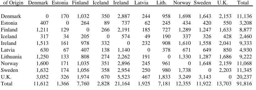
The gross flow estimates of immigration and emigration are set out in the marginal totals of Table 7 (i.e., row-sums and column-sums, respectively). The missing marginal totals for Estonia, Ireland, Latvia, Lithuania, and the United Kingdom were estimated based on the information from the Northern European countries that did provide information. Since the focus of this paper is on the place-to-place estimation of migration flows, we (for the moment) assume that these marginal estimates are reasonable and accurate. The expected international migration flows, included within the marginal totals of Table 7, were calculated based on the marginal total information. Specifically, the iterative proportional fitting
procedure was used to force a table of ones (in the off-diagonals) and zeros (in the diagonal) to fit the estimated marginal totals of the migration flow table.
Table 7. Expected international migration in Northern Europe, 1999-2000
Country
of Origin Denmark Estonia Finland Iceland Ireland Latvia Lith. Norway Sweden U.K. Total
Denmark 0 170 1,032 350 2,887 244 958 1,698 1,643 2,153 11,136 Estonia 407 0 264 89 737 62 245 434 420 550 3,208 Finland 1,211 129 0 266 2,191 185 727 1,289 1,247 1,633 8,877 Iceland 317 34 205 0 574 49 190 337 326 428 2,460 Ireland 1,513 161 978 332 0 232 908 1,610 1,558 2,041 9,333 Latvia 630 67 407 138 1,140 0 378 671 649 850 4,930 Lithuania 1,250 133 808 274 2,262 191 0 1,330 1,287 1,686 9,222 Norway 1,600 171 1,035 351 2,896 245 961 0 1,648 2,159 11,068 Sweden 1,632 174 1,056 358 2,954 250 980 1,738 0 2,203 11,345 U.K. 3,052 326 1,974 670 5,523 467 1,833 3,249 3,143 0 20,237 Total 11,612 1,366 7,760 2,828 21,164 1,925 7,181 12,355 11,922 13,703 91,816
Country of Destination
The “observed” to expected migration flow ratios are set out in Table 8 below. Note the reported international migration flows (Table 3) were proportionally adjusted to fit the adjusted column marginal totals in Table 7 before calculating the ratios. Several cells in Table 8 contain values of one. Since there were no observed values for these cells, the initial assumption was that the observed values were equal to the expected values. To improve upon this assumption, a simple regression equation based on the contiguity of countries (same as in Section 3.2.2) was used to estimate the missing ratios. Note, aside from countries that shared a border, the Scandinavian countries (i.e., Denmark, Iceland, Norway, and Sweden), and the countries of the former Soviet Union (i.e., Estonia, Latvia, and Lithuania) were considered to be neighbors. For neighboring countries, the regression model predicted a ratio of 2.1199. For non-neighboring countries, the predicted ratios were 0.2621. This regression model had an R2 of 0.346 and was significant at the 0.05 level.
Table 8. Ratios of observed to expected international migration flows in Northern Europe, 1999-2000
Country
of Origin Denmark Estonia Finland Iceland Ireland Latvia Lith. Norway Sweden U.K.
Denmark 0.0000 1.5175 0.4398 4.0495 0.1203 1.4681 0.3777 1.5284 1.0676 1.3883 Estonia 0.5830 0.0000 3.8037 0.0658 1.0000 1.0000 1.0000 0.1861 0.4992 1.0000 Finland 0.3420 2.4276 0.0000 0.1698 0.0435 0.1410 0.0163 1.0168 2.3390 1.4060 Iceland 3.6946 0.0912 0.3368 0.0000 0.0247 1.0000 0.0270 1.3030 0.9406 0.6937 Ireland 0.1625 1.0000 0.0536 0.0177 0.0000 1.0000 1.0000 0.0430 0.1021 1.0000 Latvia 0.5517 1.0000 0.1381 0.0497 1.0000 0.0000 1.0000 0.1643 0.2083 1.0000 Lithuania 0.3691 1.0000 0.0332 0.1180 1.0000 1.0000 0.0000 0.0742 0.0690 0.1304 Norway 1.8410 0.1817 1.1796 1.6807 0.0251 0.1868 0.0323 0.0000 2.6661 2.6068 Sweden 1.3011 0.3290 3.9101 1.5656 0.0802 0.1066 0.0156 3.3025 0.0000 1.0313 U.K. 1.2007 1.0000 0.3795 0.2445 3.6931 1.0000 0.0783 0.5886 0.6225 0.0000
Country of Destination
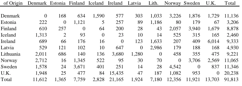
The predicted migration flows based on the estimated marginal totals (Table 7), the ratios of observed to expected flows (Table 8), and the estimated ratios based contiguity (discussed in the previous paragraph) are set out in Table 9 below. For the most part, the results appear reasonable. The only flows that may be unreasonable are the ones from Lithuania. Here, the gross flow of emigration to Northern European countries (i.e., 9,221) was most likely overestimated. This was carried out in the first stage in the modeling process --- the estimation of the marginal totals or gross flows of migration.
Table 9. Predicted international migration flows in Northern Europe, 1999-2000
Country
of Origin Denmark Estonia Finland Iceland Ireland Latvia Lith. Norway Sweden U.K. Total
Denmark 0 168 634 1,590 577 303 1,033 3,226 1,876 1,729 11,136 Estonia 222 0 1,121 5 257 89 1,186 80 179 67 3,206 Finland 610 257 0 64 200 28 43 2,057 3,940 1,679 8,878 Iceland 1,313 2 93 0 23 10 14 525 315 165 2,460 Ireland 689 66 176 16 0 123 1,633 207 409 6,014 9,333 Latvia 529 121 102 10 647 0 2,986 179 188 168 4,930 Lithuania 2,011 686 140 136 3,680 1,280 0 458 355 475 9,221 Norway 2,712 16 1,345 522 95 30 70 0 3,706 2,569 11,065 Sweden 1,578 24 3,671 401 251 14 28 4,542 0 837 11,346 U.K. 1,948 25 477 84 15,435 47 187 1,082 953 0 20,238 Total 11,612 1,365 7,759 2,828 21,165 1,924 7,180 12,356 11,921 13,703 91,813
Country of Destination
To summarize, the estimates set out in Table 9 are the result of the combination of several pieces of information. The log-linear model presented in this paper is flexible enough to deal with wide variety of place-to-place migration situations. With regard to international migration flows in Europe, there are several possible avenues for improving the estimates presented above, such as focusing on those countries with “good” data (i.e., registration-based) consistent first and then focusing on countries with relatively poor or questionable data and then those without data. Also, additional variables could be incorporated to estimate the interaction between countries. Proximity is just one factor. Other contiguity factors could include language and European Union membership, for example. Finally, it needs to be stressed that, in order to accurately model place-to-place migration flows, one needs accurate estimates of the marginal totals of a migration flow table or the gross flows of immigration and emigration for a particular migration system.
5. DISCUSSION
This paper has focused on the second stage of the estimation process and used the categorical log-linear model as the modeling platform. The main effects version of this model with an offset was used to predict the migration flows. The main effects portion ensured that the predicted values fitted the observed or estimated marginal totals. The offset portion permitted some form of spatial interaction to be included, which for the examples used in this paper, involved incorporating the available ratios of observed-to-expected migration flows and contiguity.
By considering a different interpretation of the log-linear parameters, a more
straightforward and logical solution to the estimation of origin-destination-specific migration flows was revealed. Traditionally, the parameters were interpreted in terms of geometric means or by reference to a particular category (e.g., Rogers et al. 2002; Rogers, Willekens and Raymer 2001, 2002, 2003; Willekens 1983). With an offset that includes structural zeros, the parameters of the first or last reference coding scheme are not interpretable because the reference cell is zero. With geometric mean coding, the interpretation also is not
straightforward. The interpretation of the parameters associated with both the cornered effect and effect coding schemes rely on the cell values themselves. The total sum reference
category coding scheme, on the other hand, does not. It relies on the total sum and the proportional levels represented in the row and column marginal totals. This is more useful when estimating migration flows, because one often has the marginal totals but not the cell values. The parameters of the model in this case can be used to improve the estimates.
Another development important to the estimation of origin-destination-specific flows was the identification of the offset required to perfectly predict the observed data. By
knowing that this offset represented the observed-to-expected ratios of origin-destination-specific migration flows, the focus could then be directed at the modeling of the spatial interaction. For example, the interaction parameters representing contiguity were included to improve the estimates. This identification also allowed for an easy method to convert
available data into interaction data that again improved the migration flow estimates. Migration is generally viewed as a complex phenomena that is difficult to model or incorporate into population projection models (Smith, Tayman and Swanson 2001; van der Gaag and van Wissen 1999). Unfortunately for those researchers in the area of population change, it is often the most important factor. This means it is no longer acceptable to simply ignore migration because the data are not available or are not reliable. If feasible, the missing or inadequate migration data should be collected. However, for situations in which the collection of the missing or inadequate migration data is not feasible, then an estimation procedure should be adopted and, if necessary, improved upon. The methodology provided in this paper suggests one possible avenue that is relatively robust and is based on relatively few auxiliary data.
In conclusion, estimates of place-to-place migration are needed to improve the understanding of population change, to provide more accurate population projections, and to design more effective migration policies. Toward that end, this paper has shown that is
possible to produce reasonable estimates of migration flows based on partial information. The research described herein provides new insights and improves the state-of-the-art for
estimating both internal and international migration. There are many areas where such research is needed. For example, estimates of place-to-place migration patterns could help organizations in the less developed areas of the world to construct policies that deal with
either rapid population growth or persistent decline. Historians could use this research to identify the sources of population redistribution. And, local administrators could use these methods to help predict how many jobs, schools, or hospitals their areas might require in the near future.
BIBLIOGRAPHY
Cadwallader M. 1992. Migration and residential mobility: Macro and micro approaches. Madison: The University of Wisconsin Press.
de Beer J and L van Wissen, eds. 1999. Europe: One continent, different worlds; Population scenarios for the 21st century. Dordrecht: Kluwer Academic.
Deming WE and FF Stephan. 1940. On a least squares adjustment of a sampled frequency table when the expected marginal totals are known. The Annals of Mathematical Statistics, 11(4):424-444.
Eurostat. 1999. Now-casts on international migration. Part 1: Creation of an information database. 3/1999/E/n7, European Commission, Luxembourg.
---. 2000. European social statistics: Migration. European Commission.
Flowerdew R. 1991. Poisson regression modelling of migration. In Migration models: Macro and micro approaches, Stillwell J and P Congdon, eds., pp. 92-112. London: Belhaven Press. Flowerdew R and M Aitkin. 1982. A method for fitting the gravity model based on the Poisson distribution. Journal of Regional Science, 22:191-202.
Flowerdew R and A Lovett. 1988. Fitting constrained Poisson regression models to interurban migration flows. Geographical Analysis, 20(4):297-307.
Fotheringham AS, C Brunsdon and M Charlton. 2000. Quantitative geography: Perspectives on spatial data analysis. London: Sage.
King R. 2002. Towards a new map of European migration. International Journal of Population Geography, 8:89-106.
Lowry IS. 1966. Migration and metropolitan growth: Two analytical models. San Francisco: Chandler Publishing Company.
Massey DS, J Arango, G Hugo, A Kouaouci, A Pellegrino and JE Taylor. 1998. Worlds in motion: Understanding international migration at the end of the millennium. Oxford: Clarendon Press.
Nair PS. 1985. Estimation of period-specific gross migration flows from limited data: Bi-proportional adjustment approach. Demography, 22(1):133-142.
Plane DA. 1981. Estimation of place-to-place migration flows from net migration totals: A minimum information approach. International Regional Science Review, 6(1):33-51.
Poulain M. 1994. Internal mobility in Europe: The available statistical data. Working Paper No. 17, Conference of European Statisticians, Commission of the European Communities (Eurostat), Mondorf-les-Bains, Luxembourg.
---. 1999. International migration within Europe: Towards more complete and reliable data?
Working Paper No. 37, Conference of European Statisticians, Statistical Office of the European Communities (Eurostat), Perugia, Italy.
Raymer J. 2003. The estimation of place-to-place migration flows. Dissertation. Department of Geography, University of Colorado, Boulder.
Rees PH and O Duke-Williams. 1997. Methods for estimating missing data on migrants in the 1991 British census. International Journal of Population Geography, 3:323-368.
Rogers A and LJ Castro. 1981. Model migration schedules. RR-81-30, International Institute for Applied Systems Analysis, Laxenburg, Austria.
Rogers A, FJ Willekens, JS Little and J Raymer. 2002. Describing migration spatial structure.
Papers in Regional Science, 81:29-48.
Rogers A, FJ Willekens and J Raymer. 2001. Modeling interregional migration flows: Continuity and change. Mathematical Population Studies, 9:231-263.
---. 2002. Capturing the age and spatial structures of migration. Environment and Planning A, 34:341-359.
---. 2003. Imposing age and spatial structures on inadequate migration-flow datasets. The Professional Geographer, 55(1):56-69.
Salt J. 1996. Migration pressures on Western Europe. In Europe's population in the 1990s, Coleman D, ed., pp. 92-126. Oxford: Oxford University Press.
---. 2001. Current trends in international migration in Europe. CDMG (2001) 33, Council of Europe.
Schoen R and SH Jonsson. 2003. Estimating multistate transition rates from population distributions. Demographic Research, 9(1):1-24.
Sheppard ES. 1979. Notes on spatial interaction. The Professional Geographer, 31(1):8-15. Siegel JS and CH Hamilton. 1952. Some considerations in the use of the residual method of estimating net migration. Journal of the American Statistical Association, 47:475-500. Smith SK, J Tayman and DA Swanson. 2001. State and local population projections: Methodology and analysis. New York: Kluwer Academic / Plenum.
SOPEMI. 2003. Trends in international migration: Continuous reporting system on migration (Annual report, 2002 edition). Organization for Economic Co-Operation and Development, Paris Cedex, France.
U.S. Census Bureau. 1993. 1990 County to county migration, Special Project 312. U.S. Government Printing Office, Washington, DC.
van der Gaag N and L van Wissen. 1999. Uniformity and diversity scenarios for international migration. In Europe: One continent, different worlds, de Beer J, ed., pp. 91-108. Dordrecht: Kluwer Academic.
Willekens FJ. 1977. The recovery of detailed migration patterns from aggregate data: An entropy maximizing approach. RM-77-58, International Institute for Applied Systems Analysis, Laxenburg, Austria.
---. 1980. Entropy, multiproportional adjustment and the analysis of contingency tables.
Systemi Urbani, 2:171-201.
---. 1982. Multidimensional population analysis with incomplete data. In Multidimensional mathematical demography, Land K and A Rogers, eds., pp. 43-111. New York: Academic Press.
---. 1983. Log-linear modelling of spatial interaction. Papers of the Regional Science Association, 52:187-205.
---. 1999. Modeling approaches to the indirect estimation of migration flows: From entropy to EM. Mathematical Population Studies, 7(3):239-278.
Willekens FJ, A Por and R Raquillet. 1981. Entropy, multiproportional, and quadratic techniques for inferring patterns of migration from aggregate data. In Advances in multiregional demography, RR-81-6, Rogers A, ed. Laxenburg, Austria: International Institute for Applied Systems Analysis.
Wilson AG. 1971. A family of spatial interaction models, and associated developments.
Environment and Planning, 3:1-32.