Connected Subgraph Defense Games
∗
Eleni C. Akrida
†Argyrios Deligkas
‡Themistoklis Melissourgos
§Paul G. Spirakis
¶{E.Akrida,Argyrios.Deligkas,T.Melissourgos,P.Spirakis}@liverpool.ac.uk
Abstract
We study a security game over a network played between adefenderandkattackers. Every attacker chooses, probabilistically, a node of the network to damage. The defender chooses, probabilistically as well, a connected induced subgraph of the network of λ nodes to scan and clean. Each attacker wishes to maximize the probability of escaping her cleaning by the defender. On the other hand, the goal of the defender is to maximize the expected number of attackers that she catches. This game is a generalization of the model from the seminal paper of Mavronicolas et al. [10]. We are interested in Nash equilibria of this game, as well as in characterizingdefense-optimalnetworks which allow for the bestequilibrium defense ratio, termedPrice of Defense; this is the ratio ofkover the expected number of attackers that the defender catches in equilibrium. We provide characterizations of the Nash equilibria of this game and defense-optimal networks. This allows us to show that the equilibria of the game coincide independently from the coordination or not of the attackers. In addition, we give an algorithm for computing Nash equilibria. Our algorithm requires exponential time in the worst case, but it is polynomial-time forλconstantly close to 1 orn. For the special case of tree-networks, we further refine our characterization which allows us to derive a polynomial-time algorithm for deciding whether a tree is defense-optimal and if this is the case it computes a defense-optimal Nash equilibrium. On the other hand, we prove that it is NP-hard to find a best-defense strategy if the tree is not defense-optimal. We complement this negative result with a polynomial-time constant-approximation algorithm that computes solutions that are close to optimal ones for general graphs. Finally, we provide asymptotically (almost) tight bounds for the Price of Defense for anyλ.
Keywords: Defense games, defense ratio, defense-optimal.
1
Introduction
With technology becoming a ubiquitous and integral part of our lives, we find ourselves using several different types of “computer” networks. An important issue when dealing with such networks, which are often prone to security breaches [5], is to prevent and monitor unauthorized access and misuse of the network or its accessible resources. Therefore, the study of network security has attracted a lot of attention over the years [17]. Unfortunately, such breaches are often inevitable, since some parts of a large system are expected to have weaknesses that expose them to security attacks; history has indeed shown several successful and highly-publicized such incidents [16]. Therefore, the challenge for someone trying to keep those systems and networks of computers secure is to counteract these attacks as efficiently as possible, once they occur.
To that end, inventing and studying appropriate theoretical models that capture the essence of the problem is an important line of research, ongoing for a few years now [12, 13]. In this work,
∗Supported in part by the NeST initiative of the School of EEECS of the University of Liverpool. †Department of Computer Science, University of Liverpool, Liverpool, UK.
‡Department of Computer Science, University of Liverpool, UK and Leverhulme Research Centre for Functional
Materials Design, Liverpool, UK.
§Department of Computer Science, University of Liverpool, Liverpool, UK.
¶Department of Computer Science, University of Liverpool, UK and Computer Engineering & Informatics
De-partment, University of Patras, Greece.
extending some known models for very simple cases attacks and defenses [10, 11], we introduce and analyze a more general model for a scenario of network attacks and defenses modeling it as a
defense game.
The Network Security Game. We follow the terminology established by the seminal paper of Mavronicolas et al. [11]. We consider a network whose nodes are vulnerable to infection by threats calledattackers; think of those as viruses, worms, Trojan horses or eavesdroppers [6] infecting the components of a computer network. Available to the network is a security software (or firewall), called thedefender. The defender is only able to “clean” a limited part of the network from threats that occur; the reason for the limited cleaning capacity of the defender may be, for example, the cost of purchasing a global security software. The defender seeks to protect the network as much as possible, and on the other hand, every attacker seeks to increase the likelihood of not being caught. Both the attackers and the defender make individual decisions for their positioning in the network with the aim to maximize their own objectives.
Every attacker targets (and attacks) a node chosen via her own probability distribution over the nodes of the network. The defender cleans a connected induced subgraph of the network with sizeλ, chosen via her own probability distribution over all connected induced subgraphs of the graph with
λnodes. The attack of a particular attacker is successful unless the node chosen by the attacker is incident to an edge (link) being cleaned by the defender, i.e. to an edge belonging in the induced subgraph chosen by the defender. One could equivalently think of the defender selecting a set of
λconnected nodes to defend, and an attacker is successful if and only if she attacks a node that is not being defended. Since attacks and defenses over a large computer network are self-interested procedures that seek to maximize damage and protection, respectively, it is natural to model this network security scenario as a non-cooperativestrategic game on graphs with two kinds of players:
k ≥ 1 attackers, each playing a vertex of the graph, and a single defender playing a connected induced subgraph of the graph. The (expected) payoff of an attacker is the probability that she is not caught by the defender; the (expected) payoff of the defender is the (expected) number of attackers she catches. We are interested in the Nash equilibria [14, 15] associated with this graph theoretic game, where no player can unilaterally improve her (expected) payoff by switching to another probability distribution. We are also interested in understanding and characterizing the networks that allow for a gooddefense ratio: given a strategy profile, i.e. a combination of strategies for the network entities (attackers and defender), the defense ratio of a network is the ratio of the total number of attackers over the defender’s expected payoff in that strategy profile.
1.1
Our results
In this paper we depart from and significantly extend the line of work of Mavronicolas et al. in their seminal paper [11] on defense games in graphs; we term the type of games we considerCSD games. In our model the defender is more powerful than in [11], since her power is parameterized by the size,λ, of the defended part of the network. We allow λto take values from 1 ton, while in [11] only the case whereλ= 2 was studied. We study many questions related to CSD games. We extend the notions ofdefense ratio anddefense-optimal graphs for CSD games. In fact, the defense ratio of a given graphG and a given strategy profile S of the attackers and the defender is the ratio of the number of attackers, k, over the defender’s expected payoff (the number of attackers she catches on expectation). We thoroughly investigate the notion of the defense ratio for Nash equilibria strategy profiles.
Firstly, we precisely characterize the Nash equilibria and defense-optimal graphs in CSD games. This allows us to show that, in equilibrium, the game version of k uncoordinated attackers and a single defender is equivalent to the version in which a single leader coordinates thek attackers, meaning that both versions of the game have the same defense ratio. We present an LP-based algo-rithm to compute an exact equilibrium of any given CSD game, whose running time is polynomial in nλ. Then, we focus on tree-graphs. There, we further refine our equilirbium characterization which allows us to derive a polynomial-time algorithm for deciding whether a tree is defense-optimal and, if this is the case, it computes a defense-optimal Nash equilibrium. A tree is defense-optimal if and only if it can be partitioned into n
λ disjoint sub-trees. On the other hand, we prove that
very crucial parameter for defense-optimality of a graph Gis the “best” probability with which any vertex of G is defended in a NE; we call that probabilityMaxMin probability and denote it byp∗(G). Then, for any graph G, the defense ratio in equilibrium is shown to be exactly p∗1(G).
Although it is hard to exactly compute p∗(G) even for trees, we complement this negative result with a polynomial-time constant-approximation algorithm that computes solutions that are close to the optimal ones for any λ, for any given general graph. In particular, we approximate the (best) defense ratio of any graph within a factor of 2 +λ−3
n . Finally, we provide asymptotically
tight bounds for the Price of Defense for any λ∈ ω(1)∩o(n), and almost tight bounds for any other value ofλ.
1.2
Related work
Our graph-theoretic game is a direct generalization of the defense game considered by Mavronicolas et al. [10, 11]. In the latter, the authors examined the case where the size of the defended part of the network isλ= 2, i.e. where the defender “cleans” an edge. This lead to a nice connection between equilibria and (fractional) matchings in the graph [12]. But whenλis greater than 2, one has to investigate (as we shall see here) how to sparsely cover the graph by as small a number as possible of connected induced subgraphs of size λ. This direction can be seen as an extension of fractional matchings to covers of the graph by equisized connected subgraphs. Sparse covering of graphs by connected induced subgraphs (clusters), not necessarily equisized, is a notion known to be useful also for distributed algorithms, since it affects message communication complexity [4].
In another line of work, Kearns and Ortiz [8] study Interdependent Security games in which a large number of players must make individual decisions regarding security. Each player’s safety
may depend on the actions of the entire population (in a complex way). The graph-theoretic game that we consider could be seen as a particular instance of such games with some sort of limited interdependence: the actions of the defender and an attacker are interdependent, while the actions of the attackers are not dependent on each other.
Aspnes et al. [3] consider a graph-theoretic game that models containment of the spread of viruses on a network; each node individually must choose to either install anti-virus software at some cost, or risk infection if a virus reaches it without being stopped by some intermediate node with installed anti-virus software. Aspnes et al. [3] prove several algorithmic properties for their graph-theoretic game and establish connections to a certain graph-theoretic problem called Sum-of-Squares Partition.
A game on a weighted graph with two players, thetree player and theedge player, was studied by Alon et al. [1]. At each play, the tree player chooses a spanning tree and the edge player chooses an edge of the graph, and the payoffs of the players depend on whether the chosen edge belongs in the spanning tree. Alon et al. investigate the theoretical aspects of the above game and its connections to thek-server problemand network design.
Finally, there is a long line of work on security games [2] where many scenarios are modelled using graph theoretic problems [7, 9, 18, 19].
2
Preliminaries
The game. A Connected-Subgraph Defense (CSD) game is defined by a graph G = (V, E), a
defender, k ≥ 1 attackers, and a positive integer λ. Throughout the paper, λ is considered to be a given parameter of the game. A pure strategy for the defender is any induced connected subgraph H of G with λ vertices, which we term λ-subgraph. For any λ-subgraph H of G we denote V(H) its set of vertices. Since V(H) uniquely defines an induced subgraph of G, we will use the term λ-subgraph to denote either V(H) or H. The action set of the defender is
D :={V(H)|H is aλ-subgraph ofG} and we will denote its cardinality byθ, i.e. θ :=|D|. For ease of presentation, we will also refer toD as [θ] :={1,2, . . . , θ}. A pure strategy for each of the attackers is any vertex of G. So, the action set of every attacker is V, the vertex set of G; we denoten:=|V|and we similarly refer toV also as [n].
distribution over the vertices ofG. We denote a strategy bys:= (s1, . . . , sd)∈∆d, i.e. by the
prob-ability distribution overdenumerated pure strategies, where ∆d:={x1, . . . , xd ≥0|P d
i=1xi= 1}
is the (d−1)-unit simplex. In a defense strategy q∈∆θ each pure strategyj ∈[θ] is assigned a
probabilityqj.
We say that a pure strategy of the defender, i.e. a specificλ-subgraphH ofG,covers a vertex
v∈V ifv∈V(H). A defense strategy covers a vertexv∈V if it assigns strictly positive probability to at least oneλ-subgraphH ofGwhich containsv.
Definition 1 (Vertex Probability). The vertex probability pi of vertex i∈[n], is the probability thati will be covered, formally pi :=P
j∈[θ]:i∈jqj.
Thesupportof a strategys, denoted by supp(s), is the subset of the action set that is assigned strictly positive probability.
Payoffs and Strategy profiles. A strategy profile is a tuple of strategies S = (q, t1, . . . , tk),
where q denotes the defender’s strategy and tj denotes the j-th attacker’s strategy, j ∈ [k]. A
strategy profile is pure if the support of every strategy has size one. Thepayoffof every attacker is 1 in any pure strategy profile where she does not choose a defended vertex, and 0 in all the rest. The payoff of the defender in a pure strategy profile where she defends V(H), is the number of attackers that choose a vertex inV(H). Under a strategy profile, theexpected payoffof the defender is the expected number of attackers that she catches, which we calldefense value, and the expected payoff of the attacker is the probability that she will not get caught. Abest responsestrategy for a participant is a strategy that maximizes her expected payoff, given that the strategies of the rest of the participants are fixed. ANash equilibriumis a strategy profile where all the participants are playing a best response strategy. In other words, neither the defender nor any of the attackers can increase their expected payoff by unilaterally changing their strategy.
Definition 2 (Defense Ratio). For a given graph G we define a measure of the quality of a strategy profileS, calleddefense ratio ofGand denoted DR(G, S), as the ratio of the total number of attackersk over the defense value.
In this work we are only interested in the cases whereS is an equilibrium. For a given graph, when in equilibrium, the defender’s expected payoff is unique (due to Theorem 1 and Corollary 1 (a)) and achieves theequilibrium defense ratioDR(G, S∗), whereS∗is an equilibrium. The defense strategy inS∗ which achieves this defense ratio will be termedbest-defense strategy.
Definition 3(MaxMin Probability,p∗). We call MaxMin Probabilityof a graphGthe maximum, over all defense strategies, minimum vertex probability inG, that is:
p∗(G) := max
q∈∆θ
min
i∈[n]pi.
As we will show in Lemma 1, the equilibrium defense ratio of a graph G turns out to be DR(G, S∗) = 1/p∗(G).
Definition 4(Price of Defense). ThePrice of Defense,PoD, for a given parameterλof the game, is the worst defense ratio, over all graphs, achievable in equilibrium, that is:
PoD(λ) = max
G DR(G, S
∗).
Definition 5 (Defense-Optimal Graph). For a given λ, a graph G∗ that achieves the minimum
equilibrium defense ratio over all graphs, i.e. G∗∈arg min
GDR(G, S∗), is called defense-optimal
graph.
3
Nash equilibria
In this section, we provide a characterization of Nash equilibria in CSD games, as well as important properties of their structure which prove useful for the development of our algorithms in the remainder of the paper.
Theorem 1(Equilibrium characterization). For a given graphG, in any equilibrium with support
S⊆[θ] of the defender and support Tj ⊆[n]of each attackerj ∈[k], the following conditions are
necessary and sufficient:
1. mini∈[n]pi is maximized over all defense strategies, and
2. S
j∈[k]Tj⊆V∗, whereV∗:= arg maxq∈∆θmini∈[n]pi, and
3. everys∈S has the maximum expected total number of attackers on its vertices over all pure strategies.
Proof. First we will prove that the conditions in the statement of the lemma hold in equilibrium, i.e. equilibrium is sufficient for the conditions to hold.
Condition 1. By definition, in an equilibrium the defender and each attacker have chosen a best response. Suppose that the defender has chosen some strategy q = (q1, q2, . . . , qθ) over her
action set [θ], and we will consider this strategy to be a vector variable for now. Givenq, each vertex
i∈[n] has a vertex probabilitypi. Now consider the minimum vertex probabilityp0:= mini∈[n]pi,
and the setV0⊆V consisting of the vertices with vertex probabilityp0, i.e. V0 := arg min
i∈[n]pi.
Since an attacker plays a best response, her support will be a subset ofV0; otherwise, if she assigns probability tv >0 on a vertex v /∈ V0 (withpv > p0) her expected payoff (see quantity (2)) can
be strictly increased by choosing to move all of tv to another vertex u∈ V, thus increasing her
expected payoff bytu(pv−p0). Therefore, every attacker’s support will be a subset ofV0.
Now suppose that there arek≥1 attackers and let us denote the set of attackers by [k]. We will denote bytjithe probability that the strategy of attackerj∈[k] has assigned on vertexi∈[n]. The expected payoff of the defender is:
X
i∈[n]
pi
X
j∈[k]
tji
. (1)
Since as we argued above, in an equilibrium, each attacker’s strategy has support that is subset ofV0, the expected payoff of the defender will be
X
i∈V0
pi
X
j∈[k]
tji
+
X
i∈V\V0
pi
X
j∈[k]
tji
=p
0· X
i∈V0
X
j∈[k]
tji
=p
0· X
j∈[k]
X
i∈V0 tji
=p
0·k,
where the first equality is due to the fact thatpi=p0 ∀i∈V0 andtji= 0∀i∈V \V0, and the last
equality is due to the fact that the support of any strategytj= (tj1, . . . , tji) of an attackerj∈[k]
is a subset ofV0. In an equilibrium, the defender also plays a best response, i.e. she maximizes her expected utility. Therefore, given the above quantity, the defender in an equilibrium has expected utility maxq∈∆θp
0·k, and Condition 1 of the lemma’s statement is satisfied.
Condition 2. The proof is by contradiction. Assume an equilibrium profile where the defender has strategyq= (q1, . . . , qθ) and there is an attacker,a, with strategyt= (t1, . . . , tn) whose support
includes vertexv∈[n] withpv > p0, wherep0:= mini∈[n]pi. Thena’s expected payoff is
X
i∈V i6=v
ti(1−pi) +tv(1−pv). (2)
However, a can increase her expected payoff by moving all her probability tv to a vertex v0 for
Condition 3. The proof is by contradiction. Suppose that in an equilibrium the defender has strategyq∗ ∈∆θ, where supp(q∗) :=S. According to Condition 1, this strategy achieves p∗(G),
and let us define the set V∗ := arg maxq∈∆θmini∈[n]pi. We denote by Ni the random variable
that indicates the number of attackers on vertexi∈[n], under the strategy profile determined by the strategy of the defender and each attacker. The expected utility of the defender is as in (1), or equivalently, P
i∈[n](pi·E[Ni]). Since, as argued above, in an equilibrium each attacker has
support inV∗, the defender’s expected payoff is in fact p∗·P
i∈V∗E[Ni].
For the sake of contradiction, suppose that for the expected total number of attackers on two different pure defense strategiess1∈S and s2∈[θ] it holds thatE
h P
i∈s1 Ni
i
<EhP
j∈s2Nj
i
,
and equivalently E
h P
i∈s1\s2Ni
i
<E
h P
j∈s2\s1Nj
i
. Then, the expected payoff of the defender can be strictly increased if she chooses a strategyq0= (q01, . . . , qθ0) whereqs0
1 = 0 andq
0
s2 =q
∗
s2+q
∗
s1.
In particular, when the defender playsq∗ her expected payoff is
U∗=p∗·E
X
i∈V\(s1∪s2) Ni
+p
∗·
E
X
j∈s1∩s2 Nj
+p
∗·
E
X
l∈s2\s1 Nl
+p
∗·
E
X
r∈s1\s2 Nr
,
whereas when she playsq0 it is
U0 =p∗·E
X
i∈V\(s1∪s2) Ni
+p
∗·
E
X
j∈s1∩s2 Nj
+ (p
∗+q∗
s1)·E
X
l∈s2\s1 Nl
+ (p∗−qs∗1)·E
X
r∈s1\s2 Nr
=U∗+qs∗ 1· E X
l∈s2\s1 Nl
−E
X
r∈s1\s2 Nr
> U∗,
which contradicts the equilibrium assumption. Therefore, for every pure defense strategy s1 ∈S
it holds thatE
h P
i∈s1 Ni
i
≥E
h P
j∈s2Nj
i
for everys2∈[θ].
Now we will prove that equilibrium is necessary for the three conditions of the statement to hold. Suppose that all conditions hold andp∗(G) is achieved for the defense strategy q = (q1, . . . , qθ).
We will show that the defender and each attacker play a best response.
Consider an attacker j ∈[k] with strategy t = (t1, . . . , tn) and support Tj ⊆V∗ according to
Condition 2. Her expected payoff is
X
i∈Tj
ti(1−p∗) = 1−p∗.
It suffices to consider unilateral deviations ofj to pure strategies. Any pure strategyi0 ∈Tj gives her expected payoff 1−p∗, sincepi0 =p∗ (becauseTj ⊆V∗). Any pure strategyi0 ∈V∗\Tj also
gives her expected payoff 1−p∗ for the same reason. Finally, any pure strategyi0∈V \V∗ gives her expected payoff 1−pi0 <1−p∗by the definition ofV∗. Therefore every attacker plays a best
response.
Now consider the defender with strategy q= (q1, . . . , qθ) and supportS ⊆[θ]. According to
Condition 1 of the lemma’s statement,q results to vertices ofGhaving vertex probabilityp∗. By Condition 3, for any pure defense strategy s1 ∈ S it holds that E
h P
i∈s1 Ni
i
≥ EhP
j∈s2Nj
i
for everys2∈[θ], and let us denote Nmax:=E
h P
i∈s1 Ni
i
q0= (q01, . . . , qθ0) of the defender. Her expected payoff is
U(q0) = X
j∈[θ]
qj0E
X
i∈j Ni
≤ X
j∈[θ]
qj0Nmax
=Nmax
=X
j∈S
qjE
X
i∈j Ni
=U(q),
where the penultimate equation holds due to the fact that P
j∈Sqj = 1. Therefore, q is a best
response for the defender, and the three conditions of the lemma’s statement imply a strategy profile that is an equilibrium.
Lemma 1. For any given graph G, the equilibrium defense ratio is DR(G, S∗) = p∗1(G), where
p∗(G) := max
q∈∆θmini∈[n]pi andS
∗ is an equilibrium.
Proof. As it is apparent from Theorem 1, in an equilibrium, every attacker will have in her support only vertices that are defended with probability exactlyp∗(G). Therefore, the expected number of attackers that the defender catches is p∗(G)·k. By definition of the defense ratio, DR(G, S∗) =
k p∗(G)·k =
1
p∗(G).
Corollary 1. The following hold:
(a) For a given graphG, in any equilibrium, the expected payoff of the defender and each attacker is unique.
(b) For a given graphG, in any equilibrium with supportS⊆[θ]of the defender, for everys∈S
there exists a vertexv∈ssuch thatpv=p∗(G).
(c) In any CSD game on a graph G, the problem of finding the equilibrium defense ratio (or equivalently,p∗(G)) fork≥2attackers reduces to the same problem in the game with k= 1
attacker, which is a two-player constant-sum game.
Proof. (a) By Theorem 1, in an equilibrium the defender chooses a strategy that induces proba-bilityp∗(G) to some vertex ofG(Condition 1). Also, each of the attackers has in her support
T only vertices with vertex probabilityp∗(G). Therefore, all attackers attack only such ver-tices and the expected payoff of the defender is k·p∗(G). Consider also an attacker with strategy t= (t1, t2, . . . , tn). Her expected payoff isPi∈[n]ti(1−pi), where pi is the vertex
probability of vertex i. This value is equal toP
i∈Tti(1−p∗(G)) = 1−p∗(G). Since p∗(G)
is unique for a graphG, the expected payoffs of the defender and each attacker is unique.
(b) The proof is by contradiction. Consider an equilibrium where the defender’s strategy is
q∈[θ] with supportS, and there exists a pure strategys∈S for which every vertexv ∈s
haspv > p∗(G). By Condition 2 of Theorem 1, no attacker has in her support a vertex ins.
Therefore, the defender can strictly increase her expected payoff by moving all her probability
qs>0 froms to some other pure strategys0 that contains a vertex which is in the support of some attacker.
(c) Observe that for any given graph G, the quantity p∗(G), by definition, only depends on the graph and not the number of attackers k. That is, p∗(G) is the same for every k ≥1. Lemma 1 states that in any equilibrium S∗, it is DR(G, S∗) = p∗1(G), therefore the defense
single defender and a single attacker. By definition of the game (see Section 2) the latter is a two-player constant-sum game.
The following corollary implies that coordination (resp. individual selfishness) of the attackers cannot increase the attackers’ (resp. defender’s) expected payoff in equilibrium.
Corollary 2. Every equilibrium with uncoordinated attackers (i.e. as described in Section 2) is an equilibrium with coordinated (i.e. centrally controlled) attackers, and vice versa.
Proof. Let q∗ be a best-defense strategy for the defender. Then, in any best response of any attacker, coordinated or not, every attacker plays only pure strategies that yield maximum payoff againstq∗; i.e. they play only strategies that are defended with probability p∗(G). If this was not the case, either an uncoordinated attacker could increase her payoff by unilaterally changing her strategy, or the “coordinator” could increase the payoff the attackers collectively get by dictating all the attackers to play vertices that are covered with probabilityp∗(G).
So, assume that we have an equilibrium in the uncoordinated case. This is an equilibrium for the coordinated case as well: according to Theorem 1, all attackers play vertices that are defended with probabilityp∗(G) and thus the expected collective payoff of the attackers cannot be increased, and furthermore the expected total number of attackers on the vertices of a pure strategy that is in the support of the defender is maximized over all pure defense strategies, so no unilateral deviation of the defender can increase her expected payoff.
Conversely, in any equilibrium in the coordinated setting the “coordinator” dictates all the attackers to attack vertices that are covered with probability p∗(G), satisfying Conditions 1,2 of Theorem 1. Also in the equilibrium of the coordinated setting, similarly to Condition 3 of Theorem 1, the “coordinator” will have placed the attackers in a way such that the vertices of any pure defense strategy in the support have maximum expected total number of attackers over all pure defense strategies; otherwise the defender can increase her expected payoff by neglecting a pure strategy with smaller than maximum expected total number of attackers, and move the probability assigned on that pure strategy to another one that has maximum expected total number of attackers. By Theorem 1, this is an equilibrium also for the uncoordinated setting.
The following theorem provides an algorithm for computing an equilibrium for any CSD game, whose running time is polynomial innwhenλ=cor λ=n−c, wherec is a constant natural.
Theorem 2. For some given graphGand parameterλ, there is an algorithm that computesp∗(G)
and also finds an equilibrium in time polynomial in nλ
.
Proof. Given a graphG, the number of attackersk≥1, and someλ∈ {1,2, . . . , n}, the action set
Dof the defender is constructed by the vertex sets of at most nλλ-subgraphs, so forD’s cardinality
θit holds thatθ≤ n λ
. Consider now the mixed strategyq∈∆θ of the defender, where each pure
strategyj ∈[θ] is assigned probabilityqj. Consider also the vertex probabilitypi for each vertex i ∈ [n]. According to Corollary 1 (a) and (c), the unique p∗(G) in the case of a single attacker can be used to derive an equilibrium for the case ofk≥2 attackers. Therefore, we will findp∗(G) for a single attacker, find an equilibrium for that case, and then extend this equilibrium to one in the case of k≥2 attackers. In more detail, after we find the defense strategy q∗ that maximizes mini∈[n]pi (Condition 1 of Theorem 1), i.e. yieldsp∗(G) on the setV∗:= arg maxq∈∆θmini∈[n]pi,
an equilibrium is achieved if the single attacker assigns probability 1/|V∗| to each vertex of V∗; that is because all conditions of Theorem 1 are satisfied. Then, an equilibrium fork≥2 is achieved if every attacker plays the same strategy as the single attacker; that is because again all conditions of Theorem 1 are satisfied.
The crucial observation that allows us to design such an algorithm is that we can compute
p∗(G) via a Linear Program which hasO n λ
many variables andO(n) constraints, and therefore its running time is in the worst case polynomial in nλ
, forλ∈ {2,3, . . . , n−1}. For the trivial cases λ= 1 and λ =n, D ={{i}|i ∈ V} and D = V respectively, therefore p∗(G) = 1/n and
Let us denote p∗ := p∗(G) := maxq∈∆θmini∈[n]pi. The computation of p
∗ can be done as
follows: First, consider each of the nλsubsets ofV of sizeλ, and find if it is a properλ-subgraphs ofG (i.e. connected); this can be done by running a Depth (or Breadth) First Search algorithm for each subset of size λ. If it is not, then continue with the next subset. If it is, we consider it in the action set [θ], and assign to it a variable qj which stands for its assigned probability in a general defense strategy. Now, by definition, for some vertex i ∈[n], pi =P
j∈[θ]
i∈j
qj. Therefore,
we will consider only pure strategiesj which areλ-subgraphs to create the pi’s. To compute the
minimumpiover alli’s we introduce the variablep0 and write the following set ofninequalities as
a constraint in our Linear Program:
X
j∈[θ]
i∈j
qj ≥p0 , fori∈ {1,2, . . . , n}.
The variable constraints are p0, q1, q2, . . . , qθ ≥0 and also Pθj=1qj = 1, and all of the
aforemen-tioned constraints can be written in canonical form by applying standard transformations. Finally, the objective function of the Linear Program is variablep0 and we require its maximization, which is the valuep∗.
3.1
Connections to other types of games
Although CSD games are defined as a normal form game withk+ 1 players, we can observe that there are equivalent to other well-studied types of games: polymatrix games and Stackelberg games. A polymatrix game is defined by a graph where every vertex represents a player and every edge represents a two-player game played by the endpoints of the edge. Every player has the same set of pure strategies in every game he is involved and to play the game he plays the same (mixed) strategy in every game. The payoff of every player is the sum they get from every two-player game they participate in. In a CSD game we observe the following. Firstly, the payoff of every attacker depends only on the strategy the defender plays, thus every attacker is involved only in one two-player game. In addition, all the attackers have the same set of pure strategies and they share the same payoff matrix. Similarly, the payoff the defender gets from catching an attacker depends only on the strategy the defender and this specific attacker chose. Hence, the payoff of the defender can be decomposed into a sum of payoffs fromktwo-player games. So, a CSD game can be seen as a polymatrix game where the underlying graph is a star with k leaves that correspond to the attackers and the defender is the center of the star. Although many-player polymatrix games have exponentially smaller representation size compared to the equivalent normal-form representation, we should note that this polymatrix game is of exponential size in the worst case since the defender can have exponential innpure strategies to choose from.
A Stackelberg game is an extensive form two-player game. In the first round, one of the players commits to a (mixed) strategy. In the second round, the other player chooses a best response against the committed strategy of her opponent. In a StackeIberg equilirbium the first player is playing a strategy that maximizes her expected payoff, given that the second player plays a best response (mixed strategy). The MaxMin probability p∗(G) for a CSD game on a graph G
corresponds to a Stackelberg equilibrium. By Corollary 1(c), any CSD game withk≥1 attackers has the same p∗ as that of the case with k = 1. Furthermore, as in a Stackelberg game, in the CSD game withk= 1 the defender chooses a mixed strategy that maximizes her expected payoff, given that the attacker plays a best response (mixed strategy). Therefore, when we are interested in the defense-ratio in equilibrium of a CSD game for some arbitraryk≥1, finding a Stackelberg equilibrium of the corresponding CSD game withk= 1 suffices.
4
Defense-Optimal Graphs
Theorem 3. In any defense-optimal graphG, we have that DR(G, S∗) = n λ.
Proof. First we will show that nλ is a lower bound on the Price of Defense and then prove that it is tight. According to Lemma 1, a lower bound on PoD(λ) can be found by equivalently founding an upper bound onp∗(G) over all graphsGwithnvertices. Let us show thatp∗(G)≤λ
n for everyG.
Suppose there is a graph G0 such that p∗(G0)> λn, and let us focus only on G0. Suppose also that the defender has an action set [θ] onG0. Fix the strategyq= (q1, . . . , qθ)∈∆θthat achieves p∗(G0). Then, by definition of p∗(G0), for the vertex probabilitiespi it holds thatpi > λn for all
i∈[n]. Therefore, it is
n
X
i=1
pi> λ. (3)
Also, by definition of a defense strategy, if X denotes the random variable corresponding to the number of vertices that the defender covers, then:
E[X] = θ
X
j=1
qj· |Lj|=λ ( whereLj is a λ-subgraph ofG, hence|Lj|=λ ∀j ∈[θ]). (4)
Let us introduce the indicator variablesXij, i∈[n], j ∈[θ] with value 1 if vertexi∈Lj, and
0 otherwise. Then,
E[X] = θ
X
j=1
qj n
X
i=1
Xij
=
n
X
i=1
θ
X
j=1
qjXij
=
n
X
i=1
pi (5)
> λ (by inequality (3)),
which contradicts (4).
It remains to show that the lower bound nλ on the PoD(λ) is tight. This is easy to do by showing that λ
n is a tight upper bound onp
∗(G): observe that every vertex of the line graph withn=r·λ
vertices, wherer∈N∗, can be covered with n
λ disjoint pure strategies of the defender. Therefore,
the defender can assign probability 1/(n/λ) to each pure strategy, and in that case,p∗(G) = λn.
As an intermediate corollary of Theorem 3 we get the following characterisation of defense-optimal graphs.
Corollary 3. A graph G is defense-optimal if and only if all of its vertices are defended with probability λn.
Proof. Necessity of defense-optimality is trivial: every vertex has vertex probability λ
n, therefore p∗(G) =λn, so by Theorem 3 the graph is defense-optimal.
Sufficiency of defense-optimality is also easy to see using the equations (4), (5) of the proof of Theorem 3. Suppose that the graph is defense-optimal and consider an equilibrium where the defense strategy isq= (q1, . . . , qθ). Then the sum of vertex probabilities isPni=1pi=λaccording
to the aforementioned equations. Therefore, if there exists a vertex v with vertex probability
pv > λn then there is another vertex uwith probabilitypu< nλ. This means that p∗(G)< λn, and as a result the graph is not defense-optimal which contradicts our assumption.
v1 v2 v3 v4 v5
v6
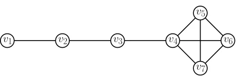
[image:11.596.198.430.95.170.2]v7
Figure 1: Heren= 7, λ= 3 andp∗(G) = 3/7 is achievable by assigning probability 3/7 to pure strategy {v1, v2, v3} and probability 1/7 to each of the pure strategies {v4, v5, v6}, {v4, v5, v7}, {v4, v6, v7},{v5, v6, v7}, so the graph is defense optimal. However, observe thatv1 cannot
partici-pate in more than one pure strategies, so in a uniform defense strategy with support of sizer, the vertex probabilitypv1 has to be 1/r(by definition of uniformity), but it also has to be 3/7. Since
r∈N, this is a contradiction.
Observation 1. All cyclic graphs are defense-optimal.
Proof. Consider an arbitrary cyclic graph G with n vertices. We will show that the graph can achieve vertex probability pi = λn for every i ∈ [n], thus by Corollary 3 it is defense-optimal. Consider the whole action set D of the defender, i.e. every path starting from a vertexi going clockwise and ending at vertex i+λ−1. Observe that there are only n such paths, therefore
θ := |D| = n. By assigning probability 1
n to each pure strategy j ∈ [θ], since each vertex is in
exactlyλpure strategies, each vertexi∈[n] has vertex probabilitypi=λ· 1θ= λn.
4.1
Tree Graphs
In this section we focus on the case where the graph is a tree. We first further refine the char-acterization of defense-optimal graphs for trees. Then, we utilise this characterisation to derive a polynomial-time algorithm that decides in polynomial time whether a given tree is defense-optimal, and if that is the case, it constructs in polynomial time a defense-optimal strategy for it. On the other hand, in the case where the tree is not defense-optimal, we show that it isNP-hard to compute a best-defense strategy for it, namely it isNP-hard to computep∗(G). We first provide Lemma 2 which will be used in our polynomial-time algorithm for checking defense-optimality on trees. Henceforth, we write that a graph is covered by a defense strategy if every vertex of the graph is covered by aλ-subgraph that is in the support of the defense strategy.
Lemma 2. A tree T is defense-optimal if and only if T can be decomposed into nλ disjoint λ -subgraphs.
Proof. (((⇒⇒⇒))) Let T be defense-optimal. We will show that the support of any best defense strategy onT must comprise of pure strategies that are disjoint λ-subgraphs which altogether cover every
v∈V. Since those are disjoint and coverT, it follows that their number is nλ in total.
Ifλ= 1 then the above trivially holds. Assume thatλ≥2 and consider a best defense strategy onT whose support comprises of a collectionLofλ-subgraphs.
Let u∈ V be a leaf ofT and let v ∈V be its parent. Any λ-subgraph inL coveringu must also cover v, sinceλ≥2. Also, any λ-subgraph in L coveringv must also cover u, otherwisepv
would be greater than pu. Now, consider the neighbors of v. For those of them that are leaves, the same must hold as holds foru, namelyv and its leaf-children must all be covered by the same exactλ-subgraph(s).
Consider the case where there is a leaf u∈ V, such that a single λ-subgraph contains u, its parentv, and all the other leaf-children ofv(and, possibly, other vertices connected tov). Then we can remove thisλ-subgraph fromLand the corresponding tree fromT. This leaves the remainder of T being a forest comprising of trees T1, . . . , Tx, each of which has a (best) defense strategy
comprising of the corresponding subset of (the remainder of) L on Ti. Notice that it must be
the case that every tree Ti, i = 1,2, . . . , x, has size at least λ (otherwise the initial collectionL
would not have coveredT). So, if there is always a leafuin some tree of the forest, such that a
vertices connected tov), we can proceed in the same fashion for each of theTi’s, always removing
aλ-subgraph fromL, and the corresponding vertices fromT, until we end up with an empty tree. This means thatLwas indeed a collection of disjoint λ-subgraphs covering T.
However, assume for the sake of contradiction that at some “iteration” the assumption does not hold, namely assume that there is a tree in the forest with no leafu, such that a singleλ-subgraph containsu, its parentv, and all the other leaf-children ofv(and, possibly, other vertices connected tov). This means that there are (at least) twoλ-subgraphs inL, namelyL1, L2, that coveru. Due
to our initial observations,u, together with its parentv and all ofv’s leaf-children are contained in both L1 and L2. Since those are different λ-subgraphs, there is a vertex z in the tree which
belongs toL2 but does not belong to L1. Sincepz=pv (due to the fact thatL is the support of
the defense-optimal strategy and Corollary 3), it must hold that there is a different λ-subgraph,
L3, which covers z but does not coverv or any of its leaf-children. If L3 also covers a vertex in
L1\L21, then there is a cycle in the tree which is a contradiction. SoL3 must not cover vertices
in L1\L2. Since L3 is different to L2, there must be a vertex z0 in the tree which belongs in
L3 but not in L2 (also not inL1). Since pz0 =pz (due to the fact that L is the support of the
defense-optimal strategy and Corollary 3), it must hold that there is a different λ-subgraph, L4,
which coversz0 but does not coverzor any of the vertices inL2. Similarly to before, ifL4 covers
a vertex inL1\L2, then there is a cycle in the tree which is a contradiction. SoL4must not cover
vertices inL1or inL2.
Proceeding in the same way, we result in contradiction since the tree has finite number of vertices and there will need to be an overlap in coverage of someLj with someLi,j > i+ 1, which would mean that there is a cycle in the tree.
Therefore, there cannot be any overlaps between theλ-subgraphs of L, meaning that L com-prises of nλ disjointλ-subgraphs which altogether coverT.
(⇐⇐⇐) Let L={L1, . . . , Ln
λ} be a collection of
n
λ disjoint λ-subgraphs that altogether cover T.
Let the defender play eachLi,i∈ {1, . . . ,nλ}, equiprobably, that is, with probability 1/ n λ
= λn. Then every vertexv ∈V is covered with probabilitypv = nλ =p∗(G), meaning thatT is defense-optimal.
With Lemma 2 in hand we can derive a polynomial-time algorithm that decides if a tree is defense-optimal, and if it is, to produce a best-defense strategy.
Theorem 4. There exists a polynomial-time algorithm that decides whether a tree is defense-optimal and produces a best-defense strategy for it, or it outputs that the tree is not defense-defense-optimal.
Proof. The algorithm works as follows. Initially, there is a pointer associated with a counter in every leaf of the tree T that moves “upwards” towards an arbitrary root of the tree. For every move of the pointer the corresponding counter increases by one. The pointer moves until one of the following happens: either the counter is equal toλ, or it reaches a vertex with degree greater of equal to 3 where it “stalls”. In the case where the counter is equal toλ, we create aλ-subgraph ofT, we delete thisλ-subgraph from the tree, we move the pointer one position upwards, and we reset the counter back to zero. If a pointer stalls at a vertex of degreed≥3, it waits until alld−1 pointers reach this vertex. Then, all these pointers are merged to a single one and a new counter is created whose value is equal to the sum of the counters of alld pointers. If this sum is more thanλ, then the algorithm returns that the graph is not defense-optimal. If this sum is less than or equal toλ, then we proceed as if there was initially only this pointer with its counter; if the new counter is equal toλ, then we create aλ-subgraph ofT and reset the counter to 0; else the pointer moves upwards and the counter increases by one. To see why the algorithm requires polynomial time, observe that we need at mostnpointers andncounters and in addition every pointer moves at mostntimes.
We now argue about the correctness of the algorithm described above. Clearly, if the algorithm does not output that the tree is not defense-optimal, it means that it partitionedTintoλ-subgraphs. So, from Lemma 2 we get thatT is defense-optimal and the uniform probability distribution over the produced partition covers every vertex with probability λ
n. It remains to argue that when the
1We useL
algorithm outputs that the graph is not defense-optimal, this is indeed the case. Consider the case where we delete aλ-subgraph of the (remaining) tree. Observe that theλ-subgraph our algorithm created deleted should be uniquely covered by thisλ-subgraph in any best-defense strategy; any other λ-subgraph would overlap with some other λ-subgraph. Hence, the deletion of such a λ -subgraph was not a “wrong” move of our algorithm and the remaining tree is defense-optimal if and only if the tree before the deletion was defense-optimal. This means that any deletion that occurred by our algorithm did not make the remaining graph non defense-optimal. So, consider the case where after a merge that occurred at vertexvwe get that the new counter isc > λ. Then, we can deduce that all the subtrees rooted atvassociated with the counters have strictly less than
λvertices. Hence, in order to cover all thec > λvertices using λ-subgraphs, at least two of these
λ-subgraphs cover vertexv. Hence, the condition of Lemma 2 is violated. But since every step of our algorithm so far was correct, it means that v cannot be covered only by one λ-subgraph. Hence, our algorithm correctly outputs that the tree is not defense-optimal.
In Theorem 4 we showed that it is easy to decide whether a tree is defense-optimal and if this is the case, it is easy to find a best-defense strategy for it. Now we prove that if a tree is not defense-optimal, then it isNP-hard to find a best-defense strategy for it.
Theorem 5. Finding a best-defense strategy in CSDgames isNP-hard, even if the graph is a tree.
Proof. We will prove the theorem by reducing from3-Partition. In an instance of 3-Partition
we are given a multiset withn positive integersa1, a2, . . . , an where n = 3mfor some m∈ N>0
and we ask whether it can be partitioned intomtripletsS1, S2, . . . , Sm such that the sum of the
numbers in each subset is equal. Lets =Pn
i=1ai. Observe then that the problem is equivalent
to asking whether there is a partition of the integers tomtriplets such that the numbers in every triplet sum up to s
m. Without loss of generality we can assume thatai< s
mfor everyi∈[n]; if this
was not the case, the problem could be trivially answered. So, given an instance of 3-Partition, we create a tree G = (V, E) with s+ 1 vertices and λ= ms + 1. The tree is created as follows. For every integer ai, we create a path with ai vertices. In addition, we create the vertex v0 and
connect it to one of the two ends of each path. We will ask whetherp∗(G)≥ 1
m.
Firstly, assume that the given instance of 3-Partitionis satisfiable. Then, givenSj we create a (ms + 1)-subgraph of G as follows. If ai ∈ Sj, then we add the corresponding path of G to the subgraph. Finally, we add vertex v0 in our (ms + 1)-subgraph and the resulting subgraph is
connected (by the construction ofG). Since the sum of ai’s equals ms, the constructed subgraph has ms + 1 vertices. If we assign probability m1 to every (ms + 1)-subgraph we get that pv ≥ 1
m for
everyv∈V.
To prove the other direction, assume that p∗(G)≥ 1
m and observe the following. Firstly, since
as we argued it isai < ms for every i ∈[n], it holds that every (ms + 1)-subgraph ofG contains vertexv0. Thus,pv0 = 1 and
P
v6=v0pv≥ s
m, since there are svertices other thanv0 and for each
one of them holds thatpv ≥ 1
m. In addition, observe that
P
v∈Vpv =λ= s
m+ 1. Hence, we get
thatpv=p∗(G) =m1 for every vertexv6=v0. In addition, observe that every pure defense strategy
that covers a leaf of this tree, covers all the vertices of the branch. Hence, for every branch of the tree, all its vertices are covered by the same set of pure strategies; if a vertexuthat is closer tov0
is covered by one strategy that does not cover the whole branch, then the leafu0 of the branch is covered with probability less thanu. So, in order for pv =p∗(G) = m1 for everyv 6=v0, it means
that there exist a (ms + 1)-subgraph that exactly covers a subset of the paths; this means that if a (ms + 1)-subgraph covers a vertex in a path, then it covers every vertex of the path. Hence, by the construction of the graph, we get that this (ms + 1)-subgraph of Gcorresponds to a subset of integers in the3-Partition instance that sum up to ms. Since, 3-Partition is NP-hard, we get that finding a best defense strategy isNP-hard.
4.2
General Graphs
We conjecture that contrary to checking defense-optimality of tree graphs and constructing a corresponding defense-optimal strategy in polynomial time, it isNP-hard to even decide whether a given (general) graph is defense-optimal.
5
Approximation algorithm for
p
∗(
G
)
We showed in the previous section that, given a graph G, it is NP-hard to find the best-defense strategy, or equivalently, to compute p∗(G). We also presented in Theorem 2 an algorithm for computing the exact value p∗(G) of a given graph G (and therefore its best defense ratio), but this algorithm has running time polynomial in the size of the input only in the cases λ = c or
λ=n−c, wherec is a constant natural. On the positive side, we present now a polynomial-time algorithm which, given a graphGofnvertices, returns a defense strategy with defense ratio which is within factor 2 + λ−3n of the best defense ratio for G. In particular, it achieves defense ratio 1/p0 ≤ 2 + λ−3n /p∗(G), where p0 = mini∈[n]pi and every pi, i ∈ [n] is the vertex probability
determined by the constructed defense strategy. We henceforth write that a collection L of λ -subgraphs covers a graph G= (V, E), if every vertex of V is covered by someλ-subgraph in L. The algorithm presented in this section returns a collectionLof at most 2n−3
λ + 1λ-subgraphs that
coversG. Therefore, the uniform defense strategy overLassigns probability at least 1/ 2n−3
λ + 1
to eachλ-subgraph.
For any collection L of λ-subgraphs and for any v ∈ V, let us denote by coverageL(v) the number ofλ-subgraphs inLwhichv belongs in. Observe that:
X
v∈V
coverageL(v) =|L| ·λ, (6)
where|L|denotes the cardinality ofL.
We first prove Lemma 3, to be used in the proof of the main theorem of this Section. We henceforth denote byV(G) andE(G) the vertex set and edge set, respectively, of some graphG.
Lemma 3. For any treeT ofnvertices, and for any λ≤n, we can find a collection Lof distinct
λ-subgraphs such that for everyv ∈ V, it holds that 1 ≤coverageL(v)≤degree(v), except maybe for (at most)λ−1 vertices, where for each of them it holds that coverageL(v) =degree(v) + 1.
Proof. We will prove the statement of the lemma by providing Algorithm 1 that takes as inputT
andλand outputs the requested collectionLofλ-subgraphs.
The algorithm starts by picking an arbitrary vertexv to serve as the root of the tree. Then it performs a Depth-First-Search (DFS) starting fromv. We will distinguish betweenvisitinga vertex andcoveringa vertex in the following way. We say that DFS visited a vertex if it considered that vertex as a candidate to be inserted to someλ-subgraph, and we say that DFS covered a vertex if it visitedandinserted the vertex at someλ-subgraph. By definition, DFS visits in a greedy manner first an uncovered child, and only if there is no such child, it visits its parent (lines 14-17, 21-24). The set-variable that keeps track of the covered vertices isS.
Starting with the root ofT, the algorithm simply visits the whole vertex set according to DFS, putting each visited vertex in the same λ-subgraph Li (starting with i = 1) (lines 18-24), and when|Li|=λ, a new emptyλ-subgraphLi+1 is picked to get filled in withλvertices (lines 26-27)
taking care of one extra thing: The first vertex that the algorithm puts in an emptyλ-subgraph
Li, i∈ {1,2, . . .} is guaranteed to be one that has not been covered by any otherλ-subgraph so far (lines 13-17). This ensures that no twoλ-subgraphs will eventually be identical.
The algorithm will not only visit all vertices inT, but also cover them. That is because there is no point where the algorithm checks whether the currently visited vertex is uncovered and then does not cover it. On the contrary, it covers every vertex that it visits, except for some already covered one in case the currentλ-subgraph is empty (lines 13-24). And since DFS by construction visits every vertex, we know that at some point the whole vertex set will be covered, or equivalently, coverageL(v) ≥ 1,∀v ∈ V. Therefore, the algorithm will eventually exit the while-loop in lines 12-29.
Now we prove that, after the algorithm terminates, every vertex v ∈ V is covered at most
degree(v) times, except for at mostλ−1 vertices that are covereddegree(v) + 1 times. Observe that DFS visits every vertex v at most degree(v) times: (a) v will be visited after its parent u
Algorithm 1Main Algorithm
Require: A tree graphT = (V, E) ofnvertices, and a naturalλ≤n.
Ensure: A collectionLof distinctλ-subgraphs that satisfies the statement of Lemma 3.
1: i, global variable. % The index of theλ-subgraphLi.
2: count, global variable. % Is 0 until the whole tree is covered, then it becomes 1 to allow for the last λ-subgraph to be completed, if it is not already.
3: S, global variable. % The set of vertices already covered by the algorithm. 4: vertex, global variable. % The vertex considered to be inserted in aλ-subgraph.
5: S← ∅
6: i←1
7: Li ← ∅
8: Pick an arbitrary vertexv ofT and consider it the root.
9: vertex←v
10: count←0
11: while count <2 do
12: while S6=V do
13: while vertex∈S do % The while-loop to ensure that the first element ofLi is
uncov-ered.
14: if vertexhas a child u /∈S then
15: vertex←u
16: else
17: vertex←parent ofvertex
18: while|Li|< λ do % The while-loop that fills in the currentλ-subgraphLi. 19: Li←Li∪ {vertex}
20: S←S∪ {vertex}
21: if vertexhas a child u /∈S then
22: vertex←u
23: else
24: vertex←parent ofvertex
25: if count <1 then
26: i←i+ 1
27: Li← ∅
28: else
29: break
30: S← ∅
31: i←i−1
32: Pick an arbitrary vertexv∈Li and consider it the root.
33: vertex←v
34: count←count+ 1
andvwill not get ever visited by its parent sincev will be covered, and alsovcannot be visited a second time by any of its children, since they can never be visited again (they can only be visited throughv sinceT is a tree). Therefore, any vertexv will be visited exactly once after its parent is visited, and at most once by each of its children, having a total of at mostdegree(v) visits. And since, as argued above, the total number of visits of a vertex is at most the number of times it will be covered, when DFS terminates, that isS =V, it will be coverageL(v)≤degree(v), for every
v∈V.
However, note that the last nonemptyλ-subgraphLi might not consist of λvertices since the
30-33). To ensure that the DFS will continue only until it fills in this current Li, the algorithm
counts the number of times that it runs the while-loop of DFS, namely lines 12-29, via the variable
count(line 34), which escapes the while-loop of DFS in case DFS has filled inLi (lines 28-29) and
terminates. Observe that in the lastλ-subgraphLi, a vertexvinserted in the last iteration of DFS (count= 1) and was not inserted in Li by the first run (count= 0) might have been covered by the first run of DFS exactlydegree(v) times, therefore when the algorithm terminates it has been covereddegree(v) + 1 times. Since by the end of the first DFS run Lihad at least one vertex, the cardinality of such vertices that are covered more times than their degree are at mostλ−1.
We can now prove the following.
Lemma 4. For any graph G of n vertices, and for any λ ≤ n, there exist (at most) 2n−3
λ + 1 λ-subgaphs ofGthat cover G.
Proof. Consider a spanning treeT of G. Then Lemma 3 applies to T. Observe that a collection
L as described in the statement of the aforementioned lemma has the same qualities for Gsince
V(T) =V(G) andE(T)⊆E(G). That is,Lis a collection of distinctλ-subgraphs ofG, such that for every v ∈V, it holds that 1 ≤ coverageL(v)≤ degree(v), except maybe for (at most) λ−1 vertices, for eachvof which it is coverageL(v) = degree(v) + 1.
Fix a particular value for λand consider a collection L of λ-subgraphs as constructed in the proof of Lemma 3. Then, by equation (6),
|L|=
P
v∈V coverageL(v)
λ ≤
P
v∈V degree(v) + (λ−1)
λ =
2(n−1)
λ +
λ−1
λ ≤
2n−3
λ + 1.
We conclude with the simple algorithm that achieves a defense strategy with defense ratio which is within factor 2 +λ−3
n of the best defense ratio for G.
Algorithm 2Approximating the best defense ratio
Require: GraphG= (V, E) ofnvertices, a naturalλ≤n.
Ensure: A defense strategy that satisfies the statement of Theorem 6.
1: Find a spanning treeT ofG.
2: Construct a collectionLofλ-subgraphs ofT as described in the proof of Lemma 3.
3: Assign probability qi= |L|1 to everyλ-subgraph inL,i= 1,2, . . . ,|L|.
4: return The above uniform defense strategy over the collectionL.
Theorem 6. Given any graphG= (V, E), Algorithm 2 computes in timeO(|E|)a defense strategy such that, for any combination of attack strategies, the resulting strategy profile S yields defense ratio DR(G, S)≤ 2 +λ−3n
·DR(G, S∗).
Proof. As argued in Lemma 4, there is a collectionLofλ-subgraphs with|L| ≤ 2n λ + 1−
3
λ which
coversG. Therefore, given the uniform defense strategy returned by Algorithm 2 (which determines the vertex probabilitypifor each vertexi) achieves a minimum vertex probabilityp0 := mini∈[n]pi
for which it holds that:
p0= 1
|L|≥
1
2n λ + 1−
3
λ
=
λ n
2 +λ−3n ≥ 1 2 + λ−3n ·p
∗(G),
where the first equality is due to the fact that any leafv∈V of the spanning treeT ofGthrough which L was created has coverageL(v) = 1, and therefore there is such a vertex v in G that is covered by exactly oneλ-subgraph; and the last inequality is due to the fact thatp∗(G)≤λ/nfor
any graphG, where p∗(G) is the MaxMin probability of G.
vertex probabilityp0 (so that the attacker is caught with minimum probability). As a result, the defender will have the minimum possible expected payoff which isp0·k. Thus, for the constructed defend strategy and any combination of attack strategies, the resulting strategy profileS yields defense ratio:
DR(G, S)≤ k
p0·k ≤
2 +λ−3
n
· 1
p∗(G) =
2 + λ−3
n
·DR(G, S∗),
where the last equality is due to Lemma 1.
With respect to the running time, notice that Step 1 of Algorithm 2 can be executed in time
O(|V|+|E(G)|) =O(|E(G)|). Step 2 can be executed in timeO(|V|+|E(T)|) =O(|V|). Finally, Step 3 can be executed in constant time. Therefore, the total running time of Algorithm 2 is
O(|E(G)|).
Corollary 4. For any graphGthere is a polynomial (in both nandλ) time approximation algo-rithm (Algoalgo-rithm 2) with approximation factor1/ 2 +λ−3n for the computation ofp∗(G).
The merit of finding a probability p0 that approximates (from below)p∗(G) for a given graph
Gthrough an algorithm such as Algorithm 2 is in guaranteeing to the defender that, no matter what the attackers play, she always “catches” at least a portion p0 of them in expectation, where the best portion is p∗(G) in an equilibrium. Algorithm 2 guarantees that the defender catches at
least 1/ 2 + λ−3
n
of the attackers in expectation.
6
Bounds on the Price of Defense
Theorem 7. ThePoD(λ) is lower bounded by j2(nλ−1)kandj2(λn+1−1)kforλeven and odd respec-tively, whenλ∈ {2,3, . . . , n−1}.
Proof. We will prove the statement by showing that for any givennandλ∈ {2,3, . . . , n−1}, there exists a graphG= (V, E) onnvertices that requires (at least) some number roughlyb=j2(λn+1−1)k ofλ-subgraphs to be covered and additionally this graph’s structure achievesp∗(G) for the uniform defense strategy, i.e. eachλ-subgraph is assigned equal probability 1/b.
The graph we construct is the following. First, consider a line graph with σ vertices, where
σ=λ
2
. Keep acentral vertexto use later, and using onlyn−1 vertices, create as manycomplete lineswith σvertices as possible, i.e. b =n−1
σ
. Create another incomplete line(if needed) with strictly less than σ vertices using the remaining ones n−1−b·σ. Now draw an edge from the central vertex to a single leaf of each of the constructed lines. For examples of the construction of
Gin each of the below three cases, see Figures 2, 3, and 4.
Consider now a defense strategy q := (q1, q2, . . . , qθ) ∈ ∆θ and the vertex probabilities p1, p2, . . . , pn it induces on the vertices ofG.
Case 1: λ is even. In this case σ =λ/2 and observe that the diameter of this graph G is equal toλ+ 1, therefore no λ-subgraph that covers a leaf of a complete line can cover a leaf of another complete line. Also, any λ-subgraph that covers a leaf of a complete line can cover the whole incomplete line. Therefore, this graph can be covered byb λ-subgraphs but no less. Assume thatqcoversG, i.e. pi>0,∀i∈[n], and let us focus on the setVcomof leaves of the complete lines
ofG, where|Vcom|=bas argued earlier, and denoteVcom by [b]. Consider the vertex probabilities pi,i∈[b], and note thatP
i∈[b]pi≤1 where strict inequality holds for the case where there exists
some pure strategyLj∈supp(q) such thatLj∩Vcom=∅. Then forp0 := mini∈[b]pi it holds that
p0 ≤1/b, otherwise pi >1/b,∀i∈[b] and thereforeP
i∈[b]pi >1 which is a contradiction. Also,
forpi= 1/b, ∀i∈[b], it isp0= 1/b, which yieldsp∗(G) := maxq∈∆θp
0 = 1/b.
Case 2: λ is odd. In this case σ= (λ+ 1)/2 and the diameter ofGequals λ+ 2, therefore noλ-subgraph that covers a leaf of a complete line can cover a leaf of another complete line.
• Subcase (a): σ−(n−1−b·σ)6= 1. Any λ-subgraph that covers a leaf of a complete line can cover the whole incomplete line. Therefore, this graph can be covered withb λ-subgraphs but no less. Following the analysis of Case 1, it isp∗(G) := maxq∈∆θp
• Subcase (b): σ−(n−1−b·σ) = 1. Noλ-subgraph that covers a leaf of a complete line can cover the leaf of the incomplete line. Therefore, this graph can be covered by b+ 1
λ-subgraphs but no less. Following similar analysis as that of Case 1, where instead ofVcom
we have Vcom∪ {vinc}wherevincis the leaf of the incomplete line, and instead ofbwe have
b+ 1, we conclude thatp∗(G) := maxq∈∆θp
0 = 1/(b+ 1).
For Case 1, and Case 2(a), since each of the leaves of thebcomplete lines have vertex probability 1/b, the defense strategy q∗ with probability qi∗ = 1/b assigned to the respective pure strategy
Li, i∈[b] that contains vertexi∈[b], yieldsp∗(G). For Case 2(b), since each of the leaves of the
b complete lines and the leafvinc of the incomplete line have vertex probability 1/b, the defense strategyq∗with probabilityqi∗= 1/(b+1) assigned to the respective pure strategyLi, i∈[b]∪{vinc}
that contains vertexi∈[b]∪ {vinc}, yieldsp∗(G).
By the above values ofp∗(G) and Lemma 1 the proof of the theorem is complete.
L1
L2
L3
[image:18.596.219.407.266.417.2]L4
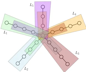
Figure 2: An example ofCase 1of Theorem 7, wheren= 15 andλ= 6. Here, graphGhasσ= 3 andb = 4. Theλ-subgraphsL1, L2, L3, L4 that constitute the support of a best-defense strategy
are shown with various colors.
L1
L2
L3
L4
Figure 3: An example of Case 2(a)of Theo-rem 7, wheren= 19 and λ= 7. Here, graph
G has σ = 4 and b = 4. The λ-subgraphs
L1, L2, L3, L4that constitute the support of a
best-defense strategy are shown with various colors.
L1
L2
L3
L4
[image:18.596.334.514.498.648.2]L5
Figure 4: An example of Case 2(b)of Theo-rem 7, where n= 20 and λ= 7. Here, graph
G has σ = 4 and b = 4. The λ-subgraphs
L1, L2, L3, L4, L5 that constitute the support
[image:18.596.109.289.517.650.2]Corollary 5. For any givennand2≤λ≤n−1, it holds thatj2(λn+1−1)k≤PoD(λ)≤ 2(n−1)+λ λ−1. Furthermore, for the trivial casesλ∈ {1, n} it isPoD(1) =nandPoD(n) = 1.
Proof. For the lower bound for 2 ≤ λ ≤ n−1, Theorem 7 shows that for given n and λ there exists a graph G with particular (very small) p∗(G), and according to Lemma 1 this yields the corresponding (great) best defense ratio. The upper bound is due to Theorem 6. For the cases
λ= 1 andλ=n, observe that the defender’s action set isD={{i}|i∈V}andD=V respectively, thereforep∗(G) = 1/n andp∗(G) = 1 respectively, and again from Lemma 1 we get the values in the statement of the corollary.
References
[1] Alon, N., Karp, R.M., Peleg, D., West, D.B.: A graph-theoretic game and its application to the k-server problem. SIAM J. Comput.24(1), 78–100 (1995)
[2] An, B., Pita, J., Shieh, E., Tambe, M., Kiekintveld, C., Marecki, J.: Guards and protect: Next generation applications of security games. ACM SIGecom Exchanges10(1), 31–34 (2011)
[3] Aspnes, J., Chang, K.L., Yampolskiy, A.: Inoculation strategies for victims of viruses and the sum-of-squares partition problem. J. Comput. Syst. Sci.72(6), 1077–1093 (2006)
[4] Attiya, H., Welch, J.: Distributed Computing: Fundamentals, Simulations and Advanced Topics. John Wiley & Sons, Inc. (2004)
[5] Cheswick, W.R., Bellovin, S.M., Rubin, A.D.: Firewalls and Internet Security: Repelling the Wily Hacker. Addison-Wesley Longman Publishing Co., Inc., Boston, MA, USA, 2 edn. (2003)
[6] Franklin, M.K., Galil, Z., Yung, M.: Eavesdropping games: a graph-theoretic approach to privacy in distributed systems. J. ACM47(2), 225–243 (2000)
[7] Jain, M., Conitzer, V., Tambe, M.: Security scheduling for real-world networks. In: Proceed-ings of the 2013 international conference on Autonomous agents and multi-agent systems. pp. 215–222. International Foundation for Autonomous Agents and Multiagent Systems (2013)
[8] Kearns, M.J., Ortiz, L.E.: Algorithms for interdependent security games. In: Advances in Neural Information Processing Systems 16 [Neural Information Processing Systems, NIPS]. pp. 561–568 (2003)
[9] Letchford, J., Conitzer, V.: Solving security games on graphs via marginal probabilities. In: Twenty-Seventh AAAI Conference on Artificial Intelligence (2013)
[10] Mavronicolas, M., Michael, L., Papadopoulou, V.G., Philippou, A., Spirakis, P.G.: The price of defense. In: Mathematical Foundations of Computer Science 2006, 31st International Sym-posium, MFCS. pp. 717–728 (2006)
[11] Mavronicolas, M., Papadopoulou, V., Philippou, A., Spirakis, P.G.: A network game with attackers and a defender. Algorithmica51(3), 315–341 (2008)
[12] Mavronicolas, M., Papadopoulou, V.G., Persiano, G., Philippou, A., Spirakis, P.G.: The price of defense and fractional matchings. In: Distributed Computing and Networking, 8th International Conference, ICDCN. pp. 115–126 (2006)
[13] Mavronicolas, M., Papadopoulou, V.G., Philippou, A., Spirakis, P.G.: A graph-theoretic network security game. In: Internet and Network Economics, First International Workshop, WINE. pp. 969–978 (2005)
[14] Nash, J.F.: Equilibrium points in n-person games. Proceedings of the National Academy of Sciences36(1), 48–49 (1950)
[16] Spafford, E.H.: The internet worm: Crisis and aftermath. Commun. ACM 32(6), 678–687 (1989)
[17] Stallings, W.: Cryptography and network security - principles and practice (3. ed.). Prentice Hall (2003)
[18] Vanˇek, O., Yin, Z., Jain, M., Boˇsansk`y, B., Tambe, M., Pˇechouˇcek, M.: Game-theoretic resource allocation for malicious packet detection in computer networks. In: Proceedings of the 11th International Conference on Autonomous Agents and Multiagent Systems-Volume 2. pp. 905–912. International Foundation for Autonomous Agents and Multiagent Systems (2012)