Efficient First-Order Temporal Logic for Infinite-State Systems

arXiv:cs/0702036v1 [cs.LO] 6 Feb 2007

Efficient First-Order Temporal Logic for Infinite-State Systems

Clare Dixon Michael Fisher Boris Konev Alexei Lisitsa Department of Computer Science, University of Liverpool

Liverpool L69 3BX, United Kingdom

{C.Dixon, M.Fisher, B.Konev, A.Lisitsa}@csc.liv.ac.uk

Abstract

In this paper we consider the specification and verification of infinite-state systems using temporal logic. In particular, we describe parameterised systems using a new variety of first-order temporal logic that is both powerful enough for this form of specification and tractable enough for practical deductive verification. Importantly, the power of the temporal language allows us to describe (and verify) asyn-chronous systems, communication delays and more complex properties such as liveness and fairness properties. These aspects appear difficult for many other approaches to infinite-state verification.

1

Introduction

First-order temporal logic (FOTL_{) has been shown to be a powerful formalism for expressing sophisticated} dynamic properties. Unfortunately, this power also leads to strong intractability. Recently, however, a fragment ofFOTL_{, called monodic} FOTL_{, has been investigated, both in terms of its theoretical [24, 22]} and practical [7, 26, 25] properties. Essentially, monodicity allows for one free variable in every temporal formula. Although clearly restrictive, this fragment has been shown to be useful in expressive description logics, infinite-state verification, and spatio-temporal logics [3, 31, 27, 20, 19].

We here develop a new temporal logic, combining decidable fragments of monodic FOTL _{[24] with} recent developments in XOR temporal logics [14], and apply this to the verification of parameterised sys-tems. We use a communicating finite state machine model of computation, and can specify not only basic synchronous, parameterised systems with instantaneous broadcast communication [17], but the powerful temporal language allows us also to specify asynchronously executing machines and more sophisticated communication properties, such as delayed delivery of messages. In addition, and in contrast to many other approaches [29, 10, 2], not only safety, but also liveness and fairness properties, can be verified through automatic deductive verification. Finally, in contrast to work on regular model checking [1] and constraint based verification using counting abstraction [17], the logical approach is both complete and decidable.

t

s

s

s

s

In describing such automata, both automata-theoretic and logical approaches may be used. While temporal logic [16] provides a clear, concise and intuitive description of the system, automate-theoretic techniques such as model checking [6] have been shown to be more useful in practice. Recently, however, a proposi-tional, linear-time temporal logic with improved deductive properties has been introduced [13, 14], provid-ing the possibility of practical deductive verification in the future. The essence of this approach is to provide an XOR constraint between key propositions. These constraints state that exactly one proposition from a XOR set can be true at any moment in time. Thus, the automaton above can be described by the following clauses which are implicitly in the scope of a ‘ ’ (‘always in the future’) operator.

1. start⇒st

2. st⇒ h(st∨sa)

3. sb ⇒ hst

4. sa⇒ hsw

5. sw ⇒ h(sw∨sb)

Here ‘ h_{’ is a temporal operator denoting ‘at the next moment’ and ‘start’ is a temporal operator which}

holds only at the initial moment in time. The inherent assumption that at any moment in time exactly one of sa,sb,storswholds, is denoted by the following.

(sa⊕sb⊕st⊕sw)

With the complexity of the decision problem (regardingsa,sb, etc) being polynomial, then the properties of

any finite collection of such automata can be tractably verified using this propositional XOR temporal logic. However, one might argue that this deductive approach, although elegant and concise, is still no better than a model checking approach, since it targets just finite collections of (finite) state machines. Thus, this naturally leads to the question of whether the XOR temporal approach can be extended to first-order temporal logics and, if so, whether a form of tractability still applies. In such an approach, we can consider infinite numbers of finite-state automata (initially, all of the same structure). Previously, we have shown that FOTL_{can be used to elegantly specify such a system, simply by assuming the argument to each predicate}

represents a particular automaton [19]. Thus, in the followingsa(X)is true if automatonXis in statesa:

1. start⇒ ∃x.st(x)

2. ∀x.(st(x)⇒ h(st(x)∨sa(x)))

3. ∀x.(sb(x)⇒ hst(x))

4. ∀x.(sa(x)⇒ hsw(x))

Thus,FOTL_{can be used to specify and verify broadcast protocols between synchronous components [17].} In this paper we define a logic, FOTLX, which allows us to not only to specify and verify systems of the above form, but also to specify and verify more sophisticated asynchronous systems, and to carry out verification with a reasonable complexity.

2

FOTLX

2.1 First-Order Temporal Logic

First-Order (discrete, linear time) Temporal Logic,FOTL_{, is an extension of classical first-order logic with} operators that deal with a discrete and linear model of time (isomorphic to the Natural Numbers,N).

Syntax. The symbols used inFOTL_are

• Predicate symbols:P0, P1, . . .each of which is of a fixed arity (null-ary predicate symbols are

propo-sitions);

• Variables:x0, x1, . . .;

• Constants: c0, c1, . . .;

• Boolean operators:∧,¬,∨,⇒,≡, true (‘true’), false (‘false’);

• First-order Quantifiers:∀(‘for all’) and∃(‘there exists’); and

• Temporal operators: (‘always in the future’), ♦(‘sometime in the future’), h_{(‘at the next}

mo-ment’), U _(until), W _{(weak until), and start (at the first moment in time).}

Although the language contains constants, neither equality nor function symbols are allowed. The set of well-formedFOTL_{-formulae is defined in the standard way [24, 7]:}

• Booleans true and false are atomicFOTL_-formulae;

• ifP is ann-ary predicate symbol andti,1 ≤i≤n, are variables or constants, thenP(t1, . . . , tn)is

an atomicFOTL_-formula;

• ifφandψareFOTL_{-formulae, so are¬φ,φ∧ψ,φ∨ψ,φ⇒ψ, andφ≡ψ;}

• ifφis anFOTL_{-formula andxis a variable, then∀xφand∃xφare}FOTL_-formulae;

• ifφandψareFOTL_{-formulae, then so are φ,}♦φ, h_φ,φU_ψ,φW_{ψ, and start.}

Mn|=atrue Mn6|=afalse

Mn|=astart iff n= 0

Mn|=aP(t1, . . . , tm) iff hIna(t1), . . . Ina(tm)i ∈In(P), where Ia

n(ti) =In(ti), iftiis a constant, andIna(ti) =a(ti), iftiis a variable

Mn|=a¬φ iff Mn6|=aφ

Mn|=aφ∧ψ iff Mn|=aφandMn|=aψ

Mn|=aφ∨ψ iff Mn|=aφorMn |=aψ

Mn|=aφ⇒ψ iff Mn|=a(¬φ∨ψ)

Mn|=aφ≡ψ iff Mn|=a((φ⇒ψ)∧(ψ⇒φ))

Mn|=a∀xφ iff Mn|=bφfor every assignmentbthat may differ fromaonly inxand such thatb(x)∈Dn

Mn|=a∃xφ iff Mn|=bφfor some assignmentbthat may differ fromaonly inxand such thatb(x)∈Dn

Mn|=a gφ iff Mn+1|=aφ;

Mn|=a♦φ iff there existsm≥nsuch thatMm|=aφ;

Mn|=a φ iff for allm≥n,Mm|=aφ;

Mn|=a(φUψ) iff there existsm≥n, such thatMm|=aψand, for alli∈N, n≤i < mimpliesMi|=

a

φ;

Mn|=a(φWψ) iff Mn|=a(φUψ)orMn|=a φ.

Figure 1: Semantics ofFOTL_.

Semantics, Intuitively, FOTL _{formulae are interpreted in first-order temporal structures which are} se-quencesM_{of worlds,}M₌M_0,M_{1, . . .with truth values in different worlds being connected via temporal}

operators.

More formally, for every moment of timen ≥0, there is a corresponding first-order structure, M_{n =}

hDn, Ini, where everyDnis a non-empty set such that whenevern < m,Dn⊆Dm, andInis an

interpre-tation of predicate and constant symbols overDn. We require that the interpretation of constants is rigid.

Thus, for every constantcand all moments of timei, j≥0, we haveIi(c) =Ij(c).

A (variable) assignmenta_{is a function from the set of individual variables to∪n∈NDn. We denote the}

set of all assignments byV_{. The set of variable assignments}V_{ncorresponding to}M_{nis a subset of the set}

of all assignments,V_n={a_∈V_|a_(x)∈Dnfor every variablex}; clearly,Vn⊆Vmifn < m.

The truth relationM_{n |=}a _{φin a structure}M_{, is defined inductively on the construction ofφonly for}

those assignmentsa_{that satisfy the condition}a _∈ V_{n. See Fig. 1 for details.} M_{is a model for a formula}

φ(orφis true inM_{) if, and only if, there exists an assignment}a_inD₀ such thatM_{0 |=}a φ. A formula is satisfiable if, and only if, it has a model. A formula is valid if, and only if, it is true in any temporal structure

M_{under any assignment}a_inD0.

The models introduced above are known as models with expanding domains sinceDn⊆Dn+1. Another

2.2 Monodicity and Monadicity

The set of valid formulae of FOTL _{is not recursively enumerable. Furthermore, it is known that even}

“small” fragments ofFOTL_{, such as the two-variable monadic fragment (where all predicates are unary),}

are not recursively enumerable [30, 24]. However, the set of valid monodic formulae is known to be finitely axiomatisable [33].

Definition 1 AnFOTL_{-formulaφis called monodic if, and only if, any subformula of the formTψ, where}

T is one of h_{, ,}♦(orψ1Tψ2, whereT is one of U, W), contains at most one free variable.

We note that the addition of either equality or function symbols to the monodic fragment generally leads to the loss of recursive enumerability [33, 8, 22]. Thus, monodicFOTL_{is expressive, yet even small}

exten-sions lead to serious problems. Further, even with its recursive enumerability, monodicFOTL_{is generally}

undecidable. To recover decidability, the easiest route is to restrict the first order part to some decidable fragment of first-order logic, such as the guarded, two-variable or monadic fragments. We here choose the latter, since monadic predicates fit well with our intended application to parameterised systems. Recall that monadicity requires that all predicates have arity of at most ‘1’. Thus, we use monadic, monodicFOTL_[7].

A practical approach to proving monodic temporal formulae is to use fine-grained temporal resolu-tion [26], which has been implemented in the theorem prover TeMP [25]. In the past, TeMP has been successfully applied to problems from several domains [21], in particular, to examples specified in the temporal logics of knowledge (the fusion of propositional linear-time temporal logic with multi-modal S5) [15, 11, 13]. From this work it is clear that monodic first-order temporal logic is an important tool for specifying complex systems. However, it is also clear that the complexity, even of monadic monodic first-order temporal logic, makes this approach difficult to use for larger applications [21, 19].

2.3 XOR Restrictions

An additional restriction we make to the above logic involves implicit XOR constraints over predicates. Such restrictions were introduced into temporal logics in [13], where the correspondence with B ¨uchi automata was described, and generalised in [14]. In both cases, the decision problem is of much better (generally, polynomial) complexity than that for the standard, unconstrained, logic. However, in these papers only propositional temporal logic was considered. We now add such an XOR constraint toFOTLX.

The set of predicate symbolsΠ ={P0, P1, . . .}, is now partitioned into a set of XOR-sets,X1,X2,. . .,

Xn, with one non-XOR setN such that

1. allXiare disjoint with each other,

2. N is disjoint with everyXi,

3. Π = n

[

j=0

Xj ∪ N, and

4. for eachXi, exactly one predicate withinXiis satisfied (for any element of the domain) at any moment

in time.

Example 1 Consider the formula

∀x.((P1(x)∨P2(x))∧(P4(x)∨P7(x)∨P8(x)))

where {P1, P2} ⊆ X1 and {P4, P7, P8} ⊆ X2. The above formula states that, for any element of the

2.4 Normal Form

To simplify our description, we will define a normal form into whichFOTLXformulae can be translated. In the following:

• X∧_ij−(x)denotes a conjunction of negated XOR predicates from the setXi;

• X∨_ij+(x)denotes a disjunction of (positive) XOR predicates from the setXi;

• N∧i(x)denotes a conjunction of non-XOR literals;

• N∨i(x)denotes a disjunction of non-XOR literals.

A step clause is defined as follows:

∧

X₁−_j(x)∧. . .

∧

X_nj−(x)∧N∧j(x)⇒

h_(X∨+

1j(x)∨. . .∨ ∨

X_nj+(x)∨N∨j(x))

A monodic temporal problem in Divided Separated Normal Form (DSNF) [7] is a quadruplehU,I,S,Ei, where:

1. the universal part,U, is a finite set of arbitrary closed first-order formulae; 2. the initial part,I, is, again, a finite set of arbitrary closed first-order formulae;

3. the step part,S, is a finite set of step clauses; and

4. the eventuality part,E, is a finite set of eventuality clauses of the form♦L(x), whereL(x)is a unary literal.

In what follows, we will not distinguish between a finite set of formulae X and the conjunction V

X of formulae within the set. With each monodic temporal problem, we associate the formula

I ∧ U ∧ ∀xS ∧ ∀xE.

Now, when we talk about particular properties of a temporal problem (e.g., satisfiability, validity, logical consequences etc) we mean properties of the associated formula.

Every monodic FOTLX formula can be translated to the normal form in satisfiability preserving way using a renaming and unwinding technique which substitutes non-atomic subformulae and replaces temporal operators by their fixed point definitions as described, for example, in [18]. A step in this transformation is the following: We recursively rename each innermost open subformula ξ(x), whose main connective is a temporal operator, byPξ(x), wherePξ(x)is a new unary predicate, and rename each innermost closed

subformulaζ, whose main connective is a temporal operator, bypζ, wherepζis a new propositional variable.

While renaming introduces new, non-XOR predicates and propositions, practical problems stemming from verification are nearly in the normal form, see Section 3.

2.5 Complexity

First-order temporal logics are notorious for being of a high complexity. Even decidable sub-fragments of monodic first-order temporal logic can be too complex for practical use. For example, satisfiability of monodic monadic FOTL _{logic is known to be} EXPSPACE_{-complete [23]. However, imposing XOR}

Theorem 1 Satisfiability of monodic monadic FOTLX formulae (in the normal form) can be decided in

2O(N1·N2·...·Nn·2Na)_{time, whereN}

1,. . . , Nnare cardinalities of the sets of XOR predicates, andNa is the

cardinality of the set of non-XOR predicates.

Before we sketch the proof of this result, we show how the XOR restrictions influence the complexity of the satisfiability problem for monadic first-order (non-temporal) logic.

Lemma 2 Satisfiability of monadic first-order formulae can be decided inNTime_{(O(n·N1·N2·. . .·Nn·2}Na_)), wherenis the length of the formula, andN1,. . . ,Nn,Naare as in Theorem 1.

Proof As in [4], Proposition 6.2.9, the non-deterministic decision procedure first guesses a structure and

then verifies that the structure is a model for the given formula. It was shown, [4], Proposition 6.2.1, Exercise 6.2.3, that if a monadic first-order formula has a model, it also has a model, whose domain is the set of all predicate colours. A predicate colour,γ, is a set of unary literals such that for every predicateP(x)from the set of all predicatesX1∪. . . , Xn∪N, eitherP(x)or¬P(x)belongs toγ. Notice that under the conditions

of the lemma, there are at mostN₁·N₂·. . .·Nn·2Na different predicate colours. Hence, the structure to

guess is ofO(N1·N2·. . .·Nn·2Na)size.

It should be clear that one can evaluate a monadic formula of the size n in a structure of the size O(N₁·N₂·. . .·Nn·2Na) in deterministic O(n·N1·N2·. . .·Nn·2Na) time. Therefore, the overall

complexity of the decision procedure isNTime_{(O(n·N1·N2·. . .·Nn·2}Na_)).

Proof [of Theorem 1, Sketch] For simplicity of presentation, we assume the formula contains no

proposi-tions. Satisfiability of a monodicFOTL_{formula is equivalent to a property of the behaviour graph for the}

formula, checkable in time polynomial in the product of the number of different predicate colours and the size of the graph, see [7], Theorem 5.15. For unrestrictedFOTL_{formulae, the size of the behaviour graph is}

double exponential in the number of predicates. We estimate now the size of the behaviour graph and time needed for its construction forFOTLXformulae.

LetΓbe a set of predicate colours andρbe a map from the set of constants,const(P), toΓ. A couple

hΓ, ρi is called a colour scheme. Nodes of the behaviour graph are colour schemes. Clearly, there are no more than 2O(N1·N2·...·Nn·2Na) _{different colour schemes. However, not every colour scheme is a node of} the behaviour graph: a colour scheme C is a node if, and only if, a monadic formula of first-order (non-temporal) logic, constructed from the givenFOTLXformula and the colour scheme itself, is satisfiable (for details see [7]). A similar first-order monadic condition determines which nodes are connected with edges. It can be seen that the size of the formula is polynomial in both cases. By Lemma 2, satisfiability of monadic first-order formulae can be decided in deterministic2O(N1·N2·...·Nn·2Na)_time.

Overall, the behaviour graph, representing all possible models, for an FOTLX formula can be

con-structed in2O(N1·N2·...·Nn·2Na)_time.

3

Infinite-State Systems

into monodicFOTL_{and used automated theorem proving in that logic to verify parameterised cache}

coher-ence protocols [10]. The model assumed not only synchronous behaviour of the communicating automata, but instantaneous broadcast.

Here we present a more general model suitable for specification of both synchronous and asynchronous systems (protocols) with (possibly) delayed broadcast and give its faithful translation into FOTLX. This not only exhibits the power of the logic but, with the improved complexity results of the previous section, provides a route towards the practical verification of temporal properties of infinite state systems.

3.1 Process Model

We begin with a description of both the asynchronous model, and the delayed broadcast approach.

Definition 2 (Protocol) A protocol, P is a tuplehQ, I,Σ, τi, where

• Qis a finite set of states;

• I ⊆Qis a set of initial states;

• Σ = ΣL∪ΣM ∪Σ¯M, where

– ΣLis a finite set of local actions; – ΣM is a finite set of broadcast actions,

i.e. “send a message”;

– Σ¯M ={σ¯|σ∈ΣM}is the set of broadcast reactions, i.e. “receive a message”;

• τ ⊆Q×Σ×Qis a transition relation that satisfies the following property

∀σ ∈ΣM.∀q ∈Q.∃q′∈Q.hq,σ, q¯ ′i ∈τ

i.e., “readiness to receive a message in any state”.

Further, we define a notion of global machine, which is a set ofnfinite automata, wherenis a parameter, each following the protocol and able to communicate with others via (possibly delayed) broadcast. To model asynchrony, we introduce a special automaton action, idle 6∈ Σ, meaning the automaton is not active and so its state does not change. At any moment an arbitrary group of automata may be idle and all non-idle automata perform their actions in accordance with the transition functionτ; different automata may perform different actions.

Definition 3 (Asynchronous Global Machine) Given a protocol, P = hQ, I,Σ, τi, the global machine

MGof dimensionnis the tuplehQMG, IMGτMG,Ei, where

• Q_MG =Q

n

• I_MG =I

n

• τMG ⊆QMG×(Σ∪ {idle})

n_×Q

MGis a transition relation that satisfies the following property

hhs₁, . . . , sni,hσ1, . . . σni,hs′₁, . . . , s′nii ∈τMG iff

∀1≤i≤n.[(σi 6=idle⇒ hsi, σi, s′ii ∈τ)

• E = 2ΣM _{is a communication environment, that is a set of possible sets of messages in transition.}

An elementG∈Q_MG×(Σ∪ {idle})

n_{× E is said to be a global configuration of the machine.}

A run of a global machineMGis a possibly infinite sequencehs1, σ1, E1i. . .hsi, σi, Eii. . .of global

configurations of MG satisfying the properties (1)–(6) listed below. In this formulation we assume si =

hsi₁, . . . , si_niandσi=hσ₁i, . . . , σ_nii.

1. s1∈In

(“initially all automata are in initial states”);

2. E1 =∅

(“initially there are no messages in transition”);

3. ∀i.hsi_{, σ}i_{, s}i+1_{i ∈τ}

MG

(“an arbitrary part of the automata can fire”;

4. ∀a∈ΣM.∀i.∀j.((σij =a)⇒ ∀k.∃l≥i.(σkl = ¯a))

(“delivery to all participants is guaranteed”);

5. ∀a∈ ΣM.∀i. ∀j. [(σij = ¯a) ⇒ (a∈ Ei)∨ ∃k. σik =a)](“one can receive only messages kept by

the environment, or sent at the same moment of time ”)

In order to formulate further requirements we introduce the following notation:

Senti ={a∈ΣM | ∃j. σji =a}

Deliveredk =

 



∃i≤k.(a∈Senti)∧

a∈ΣM (∀l.(i < l < k)→a6∈Sentl)∧ (∀j.∃l.(i≤l≤k)∧(σl

j = ¯a))

 



Then, the last requirement the run should satisfy is

6. ∀i. Ei+1= (Ei∪Senti)−Deliveredi

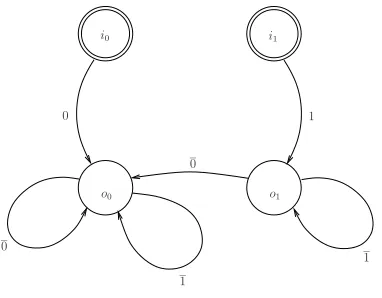
Example: Asynchronous Floodset Protocol. We illustrate the use of the above model by presenting the specification of an asynchronous FloodSet protocol in our model. This is a variant of the FloodSet algorithm with alternative decision rule (in terms of [28], p.105) designed for solution of the Consensus problem.

The setting is as follows. There arenprocesses, each having an input bit and an output bit. The processes work asynchronously, run the same algorithm and use broadcast for communication. The broadcasted messages are guaranteed to be delivered, though possibly with arbitrary delays. (The process is described graphically in Fig. 2.)

The goal of the algorithm is to eventually reach an agreement, i.e. to produce an output bit, which would be the same for all processes. It is required also that if all processes have the same input bit, that bit should be produced as an output bit.

The asynchronous FloodSet protocol we consider here is adapted from [28]. Main differences with original protocol are:

i₀ i₁

o₀ o₁

0 1

1

1 0

0

Figure 2: Asynchronous FloodSet Protocol Process.

• the original protocol assumed instantaneous message delivery, while we allow arbitrary delays in delivery; and

• although the original protocol was designed to work in the presence of crash (or fail-stop) failures, we assume, for simplicity, that there are no failures.

Because of the absence of failures the protocol is very simple and unlike the original one does not require “retransmission” of any value. We will show later (in Section 3.3) how to include the case of crash failures in the specification (and verification). Thus, the asynchronous FloodSet protocol is defined, informally, as follows.

• At the first round of computations, every process broadcasts its input bit.

• At every round the (tentative) output bit is set to the minimum value ever seen so far.

The correctness criterion for this protocol is that, eventually, the output bits of all processes will be the same.

Now we can specify the asynchronous FloodSet as a protocol hQ, I,Σ, τi, where Q = {i0, i1, o0, o1};

I = {i₀, i₁}; Σ = Σm∪Σ¯m∪ΣL withΣm = {0,1}, Σ¯m = {0¯,¯1}, ΣL = ∅. The transition relation

τ ={hi0,0, o0i,ho0,¯0, o0i,ho0,¯1, o0i,hi1,1, o1i,ho1,0¯, o0i,ho1,¯1, o1i}.

3.2 Temporal Translation

Given a protocolP =hQ, I,Σ, τi, we define its translation toFOTLXas follows.

For eachq∈Q, introduce a monadic predicate symbolPqand for eachσ ∈Σ∪ {idle}introduce a monadic

predicate symbolAσ. For eachσ∈ΣM we introduce also a propositional symbolmσ.

Intuitively, elements of the domain in the temporal representation will represent exemplars of finite automata, and the formulaPq(x)is intended to represent “automaton x is in stateq”. The formulaAσ(x)is

going to represent “automatonxperforms actionσ”. Propositionmσ will denote the fact “messageσis in

transition” (i.e. it has been sent but not all participants have received it.)

I. Each automaton either performs one of the actions available in its state, or is idle:

[∀x. Pq(x)→Aσ1(x)∨. . .∨Aσk(x)∨Aidle(x)], where{σ1, . . . σk}={σ∈Σ| ∃rhq, σ, ri ∈ τ}.

II. Action effects (non-deterministic actions): [∀xPq(x)∧Aσ(x) → hW_hq,σ,ri∈τPr(x)]for all

q∈Sandσ ∈Σ.

III. Effect of being idle: [∀xPq(x)∧Aidle(x)→ hPq(x)], for allq ∈S

IV. Initially there are no messages in the transition and all automata are in initial states: start→ ¬mσ

for allσ ∈Σmand start→ ∀xWq∈IPq(x).

V. All messages are eventually received (Guarantee of Delivery): [∃yAσ(y) → ∀x♦Aσ¯(x)], for

allσ ∈Σm.

VI. Only messages kept in the environment (are in transition), or sent at the same moment of time can be received: [∀xAσ¯(x)→mσ∨ ∃yAσ(y)]for allσ ∈Σm.

VII. Finally, for allσ∈Σm, we have the conjunction of the following formulae:

1. start→ ∀x.¬Receivedσ(x)

2. [∀x.(Aσ¯(x)∧ ¬∀y. Receivedσ(y))→ hReceivedσ(x)]

3. [∀x.(Receivedσ(x)∧ ¬∀y. Receivedσ(y)→ hReceivedσ(x)]

4. [∀x.(¬(Aσ¯(x)∨Receivedσ(x))∧ ¬∀y. Receivedσ(y))→ h¬Receivedσ(x)]

5. [∀x. Receivedσ → h¬mσ]

6. [∃x. Aσ(x)∧ ¬∀y. Receivedσ(y)→ hmσ]

7. [¬∃x. Aσ(x)∧ ¬∀y. Receivedσ(y)→(mσ ↔ hmσ]

Figure 3: Temporal Specification of Abstract Protocol Structure.

We define the temporal translation ofP, calledTP, as a conjunction of the formulae in Fig. 3. Note that, in order to define the temporal translation of requirement (6) above, (on the dynamics of environment updates) we introduce the unary predicate symbolReceivedσfor everyσ ∈Σm.

We now consider the correctness of the temporal translation. This translation of protocolPis faithful in the following sense.

Proposition 1 Given a protocol,P, and a global machine,MG, of dimensionn, then any temporal model

M1, M2, . . .ofTPwith the finite domainc1, . . . cnof sizenrepresents some runhs1, σ1, E1i. . .hsi, σi, Eii. . .

ofMGas follows:

hhs1, . . . , sni,hσ1, . . . , σni, Ei isi-th configuration of the run iff Mi |=Pq1(c1)∧. . . Pqn(cn),Mi |= Aσ1(c1)∧. . . Aσn(cn)andE ={σ ∈Σm |Mi|=mσ}

Dually, for any run ofMGthere is a temporal model of TP with a domain of sizenrepresenting this run.

3.3 Variations of the model

The above model allows various modifications and corresponding version of Proposition 1 still holds.

Determinism. The basic model allows non-deterministic actions. To specify the case of deterministic actions only, one should replace the “Action Effects” axiom in Fig. 3 by the following variant:

[∀x. Pq(x)∧Aσ(x)→ hPr(x)]

for allhq, σ, ri ∈τ

Explicit bounds on delivery. In the basic mode, no explicit bounds on delivery time are given. To intro-duce bounds one has to replace the “Guarantee of Delivery” axiom with the following one:

[∃y. Aσ(y)→ ∀x. hAσ¯(x)∨ hA¯σ(x)∨. . .∨ hnA¯σ(x)]

for allσ∈Σm and somen(representing the maximal delay).

Finite bounds on delivery. One may replace the “Guarantee of Delivery” axiom with the following one

[∃y. Aσ(y)→♦∀x. Receivedσ¯(x)]

for allσ∈Σm.

Crashes. One may replace the “Guarantee of Delivery” axiom by an axiom stating that only the messages sent by normal (non-crashed) participants will be delivered to all participants. (See [19] for examples of such specifications in aFOTL_context.)

Guarded actions. One can also extend the model with guarded actions, where action can be performed depending on global conditions in global configurations.

Returning to the FloodSet protocol, one may consider a variation of the asynchronous protocol suitable for resolving the Consensus problem in the presence of crash failures. We can modify the above setting as follows. Now, processes may fail and, from that point onward, such processes send no further messages. Note, however, that the messages sent by a process in the moment of failure may be delivered to an arbitrary subset of the non-faulty processes.

The goal of the algorithm also has to be modified, so only non-faulty processes are required to eventually reach an agreement. Thus, the FloodSet protocol considered above is modified by adding the following rule:

• At every round (later than the first), a process broadcasts any value the first time it sees it.

Now, in order to specify this protocol the variation of the model with crashes should be used. The above rule can be easily encoded in the model and we leave it as an exercise for the reader.

3.4 Verification

Now we have all the ingredients to perform the verification of parameterised protocols. Given a protocolP, we can translate it into a temporal formulaTP. For the temporal representation,χof a required correctness condition, we then check whether TP → χ is valid temporal formula. If it is valid, then the protocol is

correct for all possible values of the parameter (sizes).

Correctness conditions can, of course, be described using any legalFOTLXformula. For example, for the above FloodSet protocol(s) we have a liveness condition to verify:

♦(∀x. o0(x)∨ ∀x. o1(x))

or, alternatively

♦

(∀x.Non-faulty(x)→o0(x))∨ (∀x.Non-faulty(x)→o1(x))

in the case of a protocol working in presence of processor crashes.

While space precludes describing many further conditions, we just note that, in [19], we have demon-strated how this approach can be used to verify safety properties, i.e with χ = φ. Since we have the power of FOTLX, but with decidability results, we can also automatically verify fairness formulae of the formχ= ♦φ.

4

Concluding Remarks

In the propositional case, the incorporation of XOR constraints within temporal logics has been shown to be advantageous, not only because of the reduced complexity of the decision procedure (essentially, polynomial rather than exponential; [14]), but also because of the strong fit between the scenarios to be modelled (for example, finite-state verification) and the XOR logic [13]). The XOR constraints essentially allow us to select a set of names/propositions that must occur exclusively. In the case of verification for finite state automata, we typically consider the automaton states, or the input symbols, as being represented by such sets. Modelling a scenario thus becomes a problem of engineering suitable (combinations of) XOR sets.

In this paper, we have developed an XOR version ofFOTL_{, providing: its syntax and semantics;}

con-ditions for decidability; and detailed complexity of the decision procedure. As well as being an extension and combination of the work reported in both [7] and [14], this work forms the basis for tractable temporal reasoning over infinite state problems. In order to motivate this further, we considered a general model concerning the verification of infinite numbers of identical processes. We provide an extension of the work in [19] and [1, 2], tackling liveness properties of state systems, verification of asynchronous infinite-state systems, and varieties of communication within infinite-infinite-state systems. In particular, we are able to capture some of the more complex aspects of asynchrony and communication, together with the verification of more sophisticated liveness and fairness properties.

4.1 Related Work

The properties of first-order temporal logics have been studied, for example, in [24, 23]. Proof methods for the monodic fragment of first order-temporal logics, based on resolution or tableaux have been proposed in [7, 26, 27].

Model checking for parameterised and infinite state-systems is considered in [1]. Formulae are translated into to a B ¨uchi transducer with regular accepting states. Techniques from regular model checking are then used to search for models. This approach has been applied to several algorithms verifying safety properties and some liveness properties.

Constraint based verification using counting abstractions [9, 10, 17], provides complete procedures for checking safety properties of broadcast protocols. However, such approaches

• have theoretically non-primitive recursive upper bounds for decision procedures (although they work well for small, interesting, examples) — in our case the upper bounds are definitely primitive-recursive;

• are not suitable (or, have not been used) for asynchronous systems with delayed broadcast — it is not clear how to adapt these methods for such systems; and

• typically lead to undecidable problems if applied to liveness properties.

4.2 Future Work

Future work involves exploring further the framework described in this paper in particular the development of an implementation to prove properties of protocols in practice. Further, we would like to see if we can extend the range of systems we can tackle beyond the monodic fragment.

We also note that some of the variations we might desire to include in Section 3.3 can lead to undecid-able fragments. However, for some of these variations, we have correct although (inevitably) incomplete methods, see [19]. We wish to explore these boundaries further.

References

[1] P. A. Abdulla, B. Jonsson, M. Nilsson, J. d’Orso, and M. Saksena. Regular Model Checking for LTL(MSO). In Proc. 16th International Conference on Computer Aided Verification (CAV), volume 3114 of LNCS, pages 348–360. Springer, 2004.

[2] P. A. Abdulla, B. Jonsson, A. Rezine, and M. Saksena. Proving Liveness by Backwards Reachability. In Proc. 17th International Conference on Concurrency Theory (CONCUR), volume 4137 of LNCS, pages 95–109. Springer, 2006.

[3] A. Artale, E. Franconi, F. Wolter, and M. Zakharyaschev. A Temporal Description Logic for Rea-soning over Conceptual Schemas and Queries. In Proc. European Conference on Logics in Artificial Intelligence (JELIA), volume 2424 of LNCS, pages 98–110. Springer, 2002.

[4] E. B ¨orger, E Gr¨adel, and Yu. Gurevich. The Classical Decision Problem. Springer, 1997.

[5] J. Brotherston, A. Degtyarev, M. Fisher, and A. Lisitsa. Implementing Invariant Search via Temporal Resolution. In Proc. International Conference on Logic for Programming, Artificial Intelligence, and Reasoning (LPAR), volume 2514 of LNCS, pages 86–101. Springer Verlag, 2002.

[6] E. Clarke, O. Grumberg, and D. Peled. Model Checking. MIT Press, Dec. 1999.

[8] A. Degtyarev, M. Fisher, and A. Lisitsa. Equality and Monodic First-Order Temporal Logic. Studia Logica, 72(2):147–156, Nov. 2002.

[9] G. Delzanno. Automatic Verification of Parameterized Cache Coherence Protocols. In Proc. 12th International Conference on Computer Aided Verification (CAV), volume 1855 of LNCS, pages 53–68, 2000.

[10] G. Delzanno. Constraint-based verification of parametrized cache coherence protocols. Formal Meth-ods in System Design, 23(3):257–301, 2003.

[11] C. Dixon. Using Temporal Logics of Knowledge for Specification and Verification–a Case Study. Journal of Applied Logic, 4(1): 50-78, 2006.

[12] C. Dixon, M.C. Fern´andez-Gago, M. Fisher, and W. van der Hoek. Using Temporal Logics of Knowl-edge in the Formal Verification of Security Protocols. In Proc. International Symposium on Temporal Representation and Reasoning (TIME), pages 148–151, 2004. IEEE CS Press,

[13] C. Dixon, M. Fisher, and B. Konev. Is There a Future for Deductive Temporal Verification? In Proc. International Symposium on Temporal Representation and Reasoning (TIME), pages 11–18, 2006. IEEE CS Press.

[14] C. Dixon, M. Fisher, and B. Konev. Tractable Temporal Reasoning. In Proc. International Joint Conference on Artificial Intelligence (IJCAI). AAAI Press, 2007.

[15] C. Dixon, M. Fisher, and M. Wooldridge. Resolution for Temporal Logics of Knowledge. Journal of Logic and Computation, 8(3):345–372, 1998.

[16] E. A. Emerson. Temporal and Modal Logic. In J. van Leeuwen, editor, Handbook of Theoretical Computer Science, pages 996–1072. Elsevier, 1990.

[17] J. Esparza, A. Finkel, and R. Mayr. On the Verification of Broadcast Protocols. In Proc. 14th IEEE Symposium on Logic in Computer Science (LICS), pages 352–359. IEEE CS Press, 1999.

[18] M. Fisher, C. Dixon, and M. Peim. Clausal Temporal Resolution. ACM Transactions on Computational Logic, 2(1):12–56, Jan. 2001. ( arXiv:cs.LO/9907032)

[19] M. Fisher, B. Konev, and A. Lisitsa. Practical Infinite-state Verification with Temporal Reasoning. In Verification of Infinite State Systems and Security. IOS Press, January 2006.

[20] D. Gabelaia, R. Kontchakov, A. Kurucz, F. Wolter, and M. Zakharyaschev. On the Computational Complexity of Spatio-Temporal Logics. In Proc. 16th International Florida Artificial Intelligence Research Society Conference (FLAIRS), pages 460–464. AAAI Press, 2003.

[21] M.-C. F. Gago, U. Hustadt, C. Dixon, M. Fisher, and B. Konev. First-Order Temporal Verification in Practice. Journal of Automated Reasoning, 34(3):295–321, 2005.

[22] I. Hodkinson. Monodic Packed Fragment with Equality is Decidable. Studia Logica, 72(2):185–197, 2002.

[23] I. Hodkinson, R. Kontchakov, A. Kurucz, F. Wolter, and M. Zakharyaschev. On the Computational Complexity of Decidable Fragments of First-Order Linear Temporal Logics. In Proc. International Symposium on Temporal Representation and Reasoning (TIME), pages 91–98. IEEE CS Press, 2003. [24] I. Hodkinson, F. Wolter, and M. Zakharyashev. Decidable Fragments of First-Order Temporal Logics.

Annals of Pure and Applied Logic, 2000.

[25] U. Hustadt, B. Konev, A. Riazanov, and A. Voronkov. TeMP: A Temporal Monodic Prover. In Proc. 2nd International Joint Conference on Automated Reasoning (IJCAR), volume 3097 of LNAI, pages 326–330. Springer, 2004.

[26] B. Konev, A. Degtyarev, C. Dixon, M. Fisher, and U. Hustadt. Mechanising First-Order Temporal Resolution. Information and Computation, 199(1-2):55–86, 2005.

[28] N. Lynch. Distributed Algorithms. Morgan Kaufmann Publishers, San Mateo, CA, 1996.

[29] M. Maidl. A Unifying Model Checking Approach for Safety Properties of Parameterized Systems. LNCS, 2102:311–323, 2001.

[30] S. Merz. Decidability and Incompleteness Results for First-Order Temporal Logic of Linear Time. Journal of Applied Non-Classical Logics, 2:139–156, 1992.

[31] H. Sturm and F. Wolter. A Tableau Calculus for Temporal Description Logic: the Expanding Domain Case. Journal of Logic and Computation, 12(5):809–838, 2002.

[32] F. Wolter and M. Zakharyaschev. Decidable Fragments of First-Order Modal Logics. Journal of Symbolic Logic, 66:1415–1438, 2001.