This is a repository copy of Deriving preference-based single indices from non-preference based condition-specific instruments: Converting AQLQ into EQ5D indices.
White Rose Research Online URL for this paper: http://eprints.whiterose.ac.uk/10952/
Monograph:
Tsuchiya, A., Brazier, J., McColl, E. et al. (1 more author) (2002) Deriving
preference-based single indices from non-preference based condition-specific instruments: Converting AQLQ into EQ5D indices. Discussion Paper. (Unpublished)
HEDS Discussion Paper 02/01
Reuse
Unless indicated otherwise, fulltext items are protected by copyright with all rights reserved. The copyright exception in section 29 of the Copyright, Designs and Patents Act 1988 allows the making of a single copy solely for the purpose of non-commercial research or private study within the limits of fair dealing. The publisher or other rights-holder may allow further reproduction and re-use of this version - refer to the White Rose Research Online record for this item. Where records identify the publisher as the copyright holder, users can verify any specific terms of use on the publisher’s website.
Takedown
If you consider content in White Rose Research Online to be in breach of UK law, please notify us by
HEDS Discussion Paper 02/01
Disclaimer:
This is a Discussion Paper produced and published by the Health Economics and Decision Science (HEDS) Section at the School of Health and Related Research (ScHARR), University of Sheffield. HEDS Discussion Papers are intended to provide information and encourage discussion on a topic in advance of formal publication. They represent only the views of the authors, and do not necessarily reflect the views or approval of the sponsors.
White Rose Repository URL for this paper:
Once a version of Discussion Paper content is published in a peer-reviewed journal, this typically supersedes the Discussion Paper and readers are invited to cite the published version in preference to the original version.
Published paper
None.
The University of Sheffield
ScHARR
School of Health and Related Research
Sheffield Health Economics Group
Discussion Paper Series
May 2002
Ref: 02/1
Deriving preference-based single indices
from non-preference based condition-specific instruments:
Converting AQLQ into EQ5D indices
Aki Tsuchiya†*, John Brazier†, Elaine McColl‡, and David Parkin§
† Sheffield Health Economics Group, University of Sheffield, UK
‡ Centre for Health Services Research, University of Newcastle, UK
§ Department of Economics, City University, UK
* Corresponding author: SHEG, ScHARR, 30 Regent Street, Sheffield, S1 4DA, UK
Acknowledgements
This study has been partly funded by Novartis. We are grateful to Professor Martin Eccles for
access to quality of life data from the COGENT project, without which this analysis could not
have been completed. The COGENT study was funded by the NHS programme ‘Methods to
promote the uptake of research findings’. Tony O’Hagen and Jennifer Roberts have offered
valuable technical advice. Some of the results reported here have been presented at the
EuroQol meeting, September 2001, Copenhagen. Elaine McColl is funded by the UK
Department of Health National Primary Care Development Programme. The usual disclaimer
Abstract
Suppose that one has a clinical dataset with only non-preference-based QOL data, and that
one nevertheless would like to perform a cost/QALY analysis. This study reports on some
efforts to establish a “mapping” relationship between AQLQ (a non-preference-based QOL
instrument for asthma) and EQ5D (a preference-based generic instrument). Various methods
are described in terms of associated assumptions regarding the measurement properties of the
instruments. This is followed by empirical mapping, based on regressing EQ5D on AQLQ.
Six main regression models and two supplementary models are identified, and the regressions
carried out. Performance of each model is explored in terms of goodness of fit between
observed and predicted values, and of robustness of predictions on external data. The results
show that it is possible to predict mean EQ5D indices given AQLQ data. The general
implications for methods of mapping non-preference-based instruments onto preference-based
measures are discussed.
Key words: EQ5D, AQLQ, mapping
Introduction
What can be done when only after an important clinical trial is designed and after data
collection is completed (or only after the last chance to re-design the trial has been missed),
researchers realise the need to carry out a cost-effectiveness analysis, preferably a cost/QALY
analysis? It is very often the case that no suitable health classification instrument for deriving
preference-based single indices is incorporated, and all that is available is either a
condition-specific or generic quality of life instrument that does not have a preference-based value set to
go with it. However, suppose there is an independent dataset in which the
non-preference-based instrument used in the trial has been administered alongside a preference-non-preference-based
instrument to patients with comparable conditions to the trial patients, would it not be
possible to derive some relationship and thus an algorithm between the two types of
instruments and apply this to the trial results in order to gain some insight regarding the net
change in health gain that took place?
These are the motivations that led to this paper, which deals with the derivation of a range of
algorithms to convert non-preference information into preference-based-
single-index-equivalents. The emphasis of the paper is mostly on practicality and feasibility, what can be
done and said, rather than on the reasons why certain findings are obtained. The conversion
of non-preference-based instruments to preference-based indices should be a second best to
incorporating preference-based instruments in the trial in the first place. However, given that
some major clinical trials take years from design to completion, and that the interest in
incorporating cost/QALY studies into clinical trials is relatively recent, the kind of techniques
The paper is based on a dataset in which a disease-specific non-preference-based instrument
was administered alongside a generic preference-based instrument: these instruments were the
Asthma Quality of Life Questionnaire (AQLQ) (1, 2) and the EQ5D (3) respectively. An
algorithm for converting AQLQ information into EQ5D single indices are explored and
compared.
The AQLQ has 32 items, and each item has 7 levels, with 1 denoting extreme problems and 7
indicating no problems. The number of possible health states that can be distinguished from
each other, in theory at least, is 732 = 1.1 × 1027. The items in the AQLQ cover 4 domains
(symptoms, activities, emotions, and environment). Results can be reported in terms of
domain scores (average score across the items within each domain), or in terms of overall
score (average across all 32 items). Neither scoring system is preference-based. There are
four different versions of the instrument, two of which are relevant here: the first five items of
the original “individualised” version asks respondents to list five activities that they
personally find most limited by asthma and to indicate how much they are affected; the first
five items of the subsequent “standardised” version specifies five types of activities instead of
asking respondents to list their own particular activities. It is known that the individualised
version results in higher rates of missing data for these five items (2) Appendix 1 lists the 32
items of AQLQ.
The EQ5D has five dimensions: mobility, self-care, usual activities, pain/discomfort, and
anxiety/depression. Each dimension has one item, and each item has three levels with 1
denoting no problems and 3 denoting extreme problems. The number of theoretically
indicating the level on each dimension, or in terms of a preference-based single index number.
The latter is obtained by applying algorithms that link the 5-digit health state description with
average valuations obtained from members of the public using the time trade-off method, or
the visual analogue scale. In this study, EQ5D indices are obtained using the so-called MVH
A1 value set, derived from a population survey in the UK using 10-year time trade-offs (for
further details, see (4, 5)).
This paper is organised as follows. Section 1 reviews different ways in which this problem
may be addressed. Then section 2 describes the regression models employed in this study and
the data on which these models were applied. Section 3 reports the results of the regressions.
Section 4 is for discussion, and our conclusions regarding the feasibility and desirability of
this approach to this approach to deriving preference-based measures of health states.
1. Possible ways forward
There are four different ways in which to obtain indices from a non-preference-based
instrument such as the AQLQ, and the following is a brief exposition of each of them.
1.1. Simple transformation
The overall AQLQ score (which runs from 1-7) could be transformed to a preference-based
quality of life weight using the formula
where Q represents the preference-based quality of life weight, and A represents the overall
AQLQ score. Whilst this is the simplest approach, this is probably also the one involving the
most stringent of assumptions. These are:
(a) that the AQLQ item levels can be interpreted to represent preferences on an
interval scale, with 1 for worst health and 7 for best health,
(b) that the AQLQ items within a given domain carry equal weight,
(c) that the AQLQ domains cover all the domains of health of relevance to the
condition and its treatment,
(d) that the 4 AQLQ domains carry equal weight,
(e) that the worst state (i.e. answering 1 to all 32 items) is equivalent to being dead
and that there are no health states worse than dead, and
(f) that the best state defined by the AQLQ is equivalent to full health.
The AQLQ is designed to satisfy (c), but none of the remaining assumptions.
Furthermore, there is empirical, though inconclusive, evidence indicating that different
asthma symptoms cause different degrees of disutility to patients: Revicki and colleagues
report that patients perceive shortness of breath as being worse than coughs and wheezes
(6), while McKenzie and colleagues found that coughs and breathlessness are worse than
wheezes and chest tightness (7). Thus this approach is unlikely to be empirically robust.
1.2. A valuation study of AQLQ
A second approach is to obtain preference weights for items (i.e. individual questions) of
This approach has been successfully undertaken in three studies, one with a condition specific
measure (8) and two others involving a generic instrument, the SF-36 (9, 10). The estimation
of preference weights using this approach involves three stages. The first is to derive a health
state classification from the AQLQ that is amenable to valuation. Given that AQLQ has
millions of millions of possible combinations (or states) in all, obtaining a valuation for every
one of them is impossible. More importantly, it would be impossible for respondents to
reliably differentiate health states containing 32 pieces of information. Therefore, the health
state classification used may be reduced to the four dimensions, with appeal to assumption (b)
above, that the items within a given domain carry equal weight. If so, since there are 7 levels
on four dimensions, this reduced form will distinguish between 47 (=16,384) health states. An
alternative may be to derive a health state classification using a sample of items considered to
best represent the descriptive system of the original instrument. The second stage is to
conduct a valuation survey of a subgroup of states defined by the classification, using
standard gamble or time trade-off techniques. The third is to estimate a regression model to
establish the value set. While a valuation study of AQLQ will be an interesting enterprise, it
is unfortunately not feasible within the relevant resource constraints for our particular
exercise.
1.3. A priori mapping of AQLQ to a preference-based quality of life instrument
In this approach components of AQLQ would be associated, by judgement, to specific
domains and levels of another quality of life instrument for which preference-based weights
(c′): that the AQLQ and the preference-based measure both cover all the domains of
relevance to the condition and its treatment.
This could be done in 2 different ways: by domains, or by items. In either case, AQLQ scores
would be judged to be equivalent to a given level on a given domain of EQ5D. For instance,
scores in the range 3 to 5 on the activity domain of AQLQ might be mapped to level 2 on the
usual activities dimension of EQ5D, or levels 6 and 7 on item 14 might be equated to EQ5D
anxiety/depression level 1. Needless to say, mapping by domains involves assumption (b),
that the AQLQ items within a given domain carry equal weight, but mapping by item does
not.
A variant of this would be to deal with the problem at the level of individual patients. The
32-item profile given by a specific patient would be taken as a whole and assigned a particular
EQ5D profile, by judgement.
The main criticism for this approach is its arbitrariness (11). However, this could be
overcome by testing empirically for the appropriateness of the judgements against real data (if
there were any) to see whether or not patients who score between 3 and 5 on the AQLQ
activities domain report themselves as being on level 2 for usual activities in EQ5D. This
could lead to some kind of regression between peoples’ self-reported AQLQ and EQ5D.
Pushing this further is equivalent to the empirical mapping discussed in the following section.
The essence of this approach is to explore the relationship between the two instruments by
regression analyses. This requires a real dataset in which patients have responded to an
appropriate quality of life instrument (which will be the dependent variable in the regressions)
alongside AQLQ (scores of which will be the independent variables). This is the method
employed in this paper, and is explained in more detail in the following section.
2. Methods
2.1. The regression models
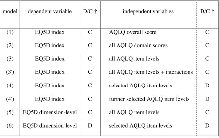
As summarised in table 1, there are at least six additive regression models, and two
supplementary models, which could be used to estimate the relationship between AQLQ and
EQ5D. Each is briefly explained. The notation used is as follows, where figures in square
brackets indicate the potential range:
Q: the preference-based EQ5D index [-0.59,1]
A: the AQLQ overall score [1,7]
Ad: the score of an AQLQ domain [1,7], where d = S, A, Em, Ev,
Ai: the level of an AQLQ item [1,7], where i = 1, 2, … 32
Ai.x: a dummy variable that = 1 when the level of an AQLQ item i is x
Ed: the level of an EQ5D dimension [1,3], where d = M, SC, UA, PD, AD
All regressions are run using STATA version 6. Rather arbitrarily, “level” is used for AQLQ
domains and overall scores, ie. for continuous data. Scores are always treated as continuous
variables in the regressions, but levels can be treated as either continuous or discrete variables.
(1) Q = a + $ + u,
(2) Q = a + 1AS + 2AA + 3AEm + 4AEv + u,
(3) Q = a + 1A1 + 2A2 + … 32A32 + u.
These 3 models are estimated using ordinary least squares (OLS), and the independent
variables are treated as continuous. Model (1) requires assumptions (a) (b) (c') and (d), while
model (2) requires (a) (b) and (c'), and model (3) requires (a) and (c').
(3'): Q = a + 1A1 + … 32A32 +i.iAiAi + … i.nAiAn + … n.nAnAn + u,
where the subscript i.n represents item i and item n of AQLQ. This is supplementary to
model (3), and additional interaction terms are included. In this study, the independent
variables (i to n) used to form the interaction terms are selected according to the results of
model (3) based on the criteria: (i) the sign for the estimator is positive (a positive sign is
expected, since a higher AQLQ level should be associated with better quality of life and
larger EQ5D indices), and (ii) its p value is less than 0.01. The latter criterion is arbitrary.
The products of pairs of these items and squares of these items are added to the main effects
model and estimated using OLS. Like model (3), this model requires assumption (a) and (c').
(4) Q = a + i.2Ai.2 + i.3Ai.3 + …i.7Ai.7 + … n.7An.7 + u,
where the subscript i.x represents level x on item i of AQLQ. The independent variables are a
selected subset of the AQLQ items. In this study, this subset is selected according to the
results of model (3) based on the criteria: (i) the sign for the estimator is positive, as expected,
counterpart in model (3'). This model continues to use OLS, but now the independent
variables are treated as categorical variables. Thus, the number of independent variables will
be 6 times the number of items selected (because each item has 7 levels). This model requires
assumption (c') alone.
(4') Q = a + i.2Ai.2 + i.3Ai.3 + …i.7Ai.7 + … m.7Am.7 + u, m < n.
Here, the independent variables are restricted further by applying the same criteria again.
Whole items will be excluded, as opposed to excluding individual variables. This is because
each variable represents different levels within a given item, and it becomes difficult to
interpret if not all the levels of a given item were either included or excluded as one set. An
alternative at this stage would be to merge levels by imposing equality constraints on the
coefficients. This was not done in this study.
(5) regress the five EQ5D dimensions on the 32 AQLQ item levels so that
EM = a + 1A1 + 2A2 + … 32A32 + u,
ESC = a + 1A1 + 2A2 + … 32A32 + u,
EUA =
…
Again, OLS is used, and both the dependent and the independent variables are treated as
continuous. Five regression functions, each for one of the EQ5D dimensions, are estimated.
The required assumptions are (a) and (c'). Further, note that, while on the one hand the EQ5D
algorithm for obtaining the preference-based single index is based on a series of coefficients
to be applied to discrete numbers representing the level on different EQ5D dimensions, on the
in terms of goodness of fit cannot be tested. Rather, the objective of this model is to enable
the selection of the independent variables used in the next model. In addition, this is the best
model to explore empirically the relationship between the descriptive content of the two
instruments, which is explored in section 5 below.
(6) regress the 5 EQ5D dimensions on a subset of the AQLQ item levels so that
EM = a + iAi + jAj + … nAn + u,
ESC = a + iAi + jAj + … nAn + u,
EUA =
…
As in model (5), there is one regression function for each of the five EQ5D dimensions.
Instead of OLS, multinomial logistic regressions are used where the levels within a given
EQ5D dimension are treated as categorical variables (in other words, the dependent variable
is now discrete). The independent variables are also treated as categorical, and are selected
based on the results of model (5), while the selection criteria are the same as those used for
model (4). The subset of independent variables will not necessarily be the same across the 5
EQ5D dimensions. The required assumption is (c') alone.
2.2. The goodness of fit
Given that the objective of the exercise is not to explain the relationship between AQLQ and
EQ5D, the size of R2 is not an indicator of much importance (although it is reported). The
objective of the exercise is to predict the EQ5D index of a patient with a given AQLQ profile.
Therefore the error of the prediction, or the goodness of the fit is taken as the criterion of
smaller this value, the better is the performance. Scatter plots between directly derived EQ5D
indices and EQ5D indices predicted from the models will be examined (mostly not shown due
to space constraints, but available from the corresponding author on request). The range of
the predicted values, and Pearson’s correlation coefficients between the observed and the
predicted EQ5D indices are also reported.
While obtaining predicted EQ5D indices for the OLS models is straightforward, doing this for
model (6) requires some explanation. The predictions generated from model (6) are the
probability that a given respondent has a given level on each of the EQ5D dimensions (eg. the
probability of level 1 for mobility, the probability of level 2 for mobility, etc). Based on these,
there are two ways in which to calculate an EQ5D index. The first, “indirect” way, looks at
these probabilities and determines the level for each of the five dimensions by choosing the
level with the highest associated probability. This leads to the identification of an EQ5D
profile, to which the value set can be applied. Since this approach makes no distinction
between a probability distribution of 34%-33%-33% for the three levels of a given dimension
and one of 90%-5%-5%, the method does not utilise all available information. The second,
“direct” way, uses the probabilities for different dimensions and levels, including the
interaction term for extreme problems, and combines these with the value set to calculate an
expected EQ5D index. The shortcoming of this latter method is that it becomes almost
impossible to have a predicted EQ5D index of 1.00. Given the observed distribution of
EQ5D responses in the estimation dataset (presented below), where a substantial proportion
of respondents had EQ5D of 11111, the choice was made to obtain predicted values for model
2.3. Robustness
The goodness of fit above is obtained for “within-sample” predictions. In other words, the
dataset on which the model is estimated and the dataset on which the predictions are fitted are
the same. In order to explore the robustness of the model, “out-of-sample” predictions are
also obtained. Here, the data on which the predictions are fitted are not the same as the data
on which the model is estimated. 75% of the whole sample is randomly selected, the
regressions run, and then the predictions calculated for the remaining 25% of the sample.
This is repeated three times on different splits of the whole sample, and MSE is reported for
each.
2.4. The data
The data used in this study comes from a randomised controlled trial that looked into the
effectiveness of computerised decision support in primary care, covering a wide range of
patients with asthma. A sample of 3000 patients was identified from general practice
morbidity and prescribing registers and were surveyed in three rounds roughly 12 months
apart (n diminishes with round). Amongst other information, AQLQ and EQ5D were
collected using posted questionnaires. The original AQLQ was used for round 1, and due to
significant levels of item non-response to the individualised items in round 1, the standardised
AQLQ was used for rounds 2 and 3. For further details, see Eccles et al (12).
There are three datasets to work on:
“R1”: all responses to round 1; n = 3059; AQLQ items 1-5 are individualised,
“R123”: items 6-32 from rounds 1,2, and 3; n = 6939 (items 1-5 are excluded because of
the lack of comparability of data from round 1 vs. rounds 2 and 3).
Across the three rounds, each EQ5D dimension has around 2-3% missing data. There are
more missing data in AQLQ: 12-24% for items 5 of original AQLQ; and 2-11% for items
1-5 of the standardised questionnaire. For other items, 1-4% of responses are missing.
Mean EQ5D index in dataset R123 is 0.73. 27% of respondents report full health (11111).
Other common states are 11121 (10%), 21222 (7%), 11112 and 11122 (6% each). 75% of
respondents do not report any impairment at level 3 on any dimension. Further, some EQ5D
dimensions have very few patients in level 3 (0.2% for mobility, 0.3% for self care).
Mean AQLQ overall score in dataset R123 is 4.94. Domain scores range from 4.81
(environment) to 5.10 (activities). The distribution of AQLQ responses is somewhat more
uniform, so that the least frequently endorsed level (which always is the worst level) usually
has over 3% responses, and at the least 1%. 91-97% of respondents (depending on dataset)
have a “unique” response so that there is no other respondent sharing the same AQLQ
response across all 32 items. Around 1% have one other respondent with the same response
profile. 1-3% of respondents have no problems across any of the 32 AQLQ items (i.e.
endorse level 7 on all 32 items).
The overall skewness of the data from both instruments is problematic. It means that data are
thin regarding the more severe health states, and the ability of the model to predict with
distribution before running the regressions. However, given that the objective of this exercise
is to estimate a model for prediction, as opposed to explanation, and given also that the same
skew of the AQLQ responses may not apply to the data to which the mapping algorithm is
applied, data are not transformed.
2.5. The choice of regression models
There are three issues here: the inclusion of patient background characteristics, the use of
generalised linear models, and the use of random or fixed effects models.
The independent variables of the regression models used are limited to AQLQ scores, and
exclude patient background characteristics, such as age and sex, despite the possibility of
misspecification. Preliminary analyses using dataset R1 and models (1) (2) (3) and (4)
indicate that when age, age squared, and sex are included, these variables result in statistically
significant coefficients. However, the other coefficients are hardly affected (maximum,
minimum, and average change are: 0.010, -0.007, 0.000, and average absolute change is
0.000). Note moreover that, given that the final objective of the exercise is to apply the
estimated mapping algorithm to trial data and to calculate net benefit of treatment, whatever
variables included in the additive model that do not change between baseline and follow up
observations will simply be cancelled out. Therefore, background characteristics are
deliberately excluded from the regression models.
Given that the EQ5D indices used as the dependent variable in the OLS models are bounded
to 1.00, the use of simple linear models risks the predicted values being larger that this limit.
transformed into an s-shaped non-linear variable that approaches 1, but does not reach it. The
obvious shortcoming of this in our context is that there are many responses with observed
EQ5D index of 1.00, and the transformation will imply dropping these observations (because
the transformed values approaches infinity). This can be accommodated by standardising the
raw EQ5D indices to the range [0, 1], based on an artificial range, say, [-0.5, +1.1], and then
transforming this. A preliminary analysis was carried out using dataset R1 and models (1) (2)
(3) and (4), and applying a logit transformation to the thus standardised EQ5D indices. In
terms of Pearson’s correlation between the observed and predicted EQ5D indices,
performance of GLM and the simple linear model are roughly the same (correlation
coefficients of GLM are better by less than 1%). However, GLM for models (1) and (2) do
markedly worse than the simple linear model in terms of MSE (>0.08 as opposed to <0.05),
and maximum predicted value for those with EQ5D index = 1 is much smaller (around 0.65
as opposed to 1.00 ± 0.02). With models (3) and (4), GLM is comparable to the simple linear
regression, but not better. Given the additional complication, the arbitrary nature of the
standardisation and the transformation, and the fact that the maximum predicted EQ5D
indices of the simple linear models hardly exceed 1.00, the associated benefits of GLM do not
seem to outweigh its costs. Therefore the decision was made not to use GLM.
Finally, given that the datasets R23 and R123 are composed of repeated observations, there is
theoretical scope to consider the use of either random or fixed effect models. Indeed, using
dataset R123 and model (3), the Breusch-Pagen test indicates that there are individual effects.
A subsequent Hausman test rules out the use of fixed effects model in favour of the random
effects model. However, on the one hand, a requirement for the use of random effects models
independent variables being self-reported AQLQ, the two are unlikely to be independent.
Therefore, the decision was made to not to use random or fixed effects models.
3. Results
3.1. Regression coefficients, p-values and MSE.
Model (1)
This indicates a positive correlation between EQ5D index and AQLQ overall score, and there
is very little difference in the coefficients across the three datasets. Adjusted R2 = 0.33 for all
datasets, and MSE is 0.049 to 0.053.
overall 0.12, p < 0.01,
Model (2):
As already outlined, AQLQ domain scores should be positively correlated to EQ5D indices
(i.e. the larger the score the better the quality of life). AQLQ symptoms and activities
domains have expected signs ( > 0), but emotions and environment domains have the
opposite sign and p < 0.1, except for emotions for dataset R1 (where >0 but p = 0.77).
Adjusted R2 across the three datasets ranges from 0.35 to 0.37, and MSE ranges from 0.044 to
0.049.
symptom 0.04 to 0.05, p < 0.01
activities 0.10 to 0.11, p < 0.01
environment -0.03, p < 0.01
Model (3):
There are certain AQLQ items that persistently have the reverse, or wrong sign ( < 0) with p
< 0.1, across the three datasets. The “well behaved” items ( > 0 and p < 0.1 in at least two
datasets) are:
Symptoms: 6, 16, 29, 30
Activities: 3, 5, 25, 28, 31, 32
Emotions: 15, 27
Environment: 26
The “badly behaved” items ( < 0 and p < 0.1 in at least two datasets) are:
Symptoms: none
Activities: 22, 24
Emotions: 21
Environment: 23
There are larger differences across datasets than with models (1) and (2), which is expected,
due to the treatment of items 1-5. Adjusted R2 across the three datasets is in the range 0.36 to
0.39 and MSE ranges from 0.042 to 0.048.
Model (3')
The AQLQ items selected to form the interaction terms are as follows:
dataset R1: 3, 5, 25, 27, 31
The five items selected for dataset R1 form 15 interaction independent variables (item 3
squared, item 5 squared, …; product of items 3 and 5, product of items 3 and 25, …), and
similarly, there are 15 interaction terms for dataset R23, and 28 for dataset R123. Of these,
six, six and 14 items respectively had regression coefficients with the expected sign ( > 0).
For dataset R1 none of these had p < 0.1, for R23 two (product of items 2 and 4, product of
items 2 and 16) had p < 0.1, and for R123 three (square of item 29, product of items 16 and 27,
and product of items 16 and 29) had p < 0.1. Adjusted R2 for the three datasets is between
0.37 and 0.40, and MSE is between 0.041 and 0.047.
Model (4):
The AQLQ items selected for this model based on model (3) are:
dataset R1: 1, 3, 5, 6, 25, 26, 27, 29, 31, 32
dataset R23: 2, 3, 4, 5, 6, 14, 16, 25, 28, 30, 31
dataset R123: 6, 16, 25, 26, 27, 28, 29, 30, 31, 32
Not many coefficients have the wrong sign: there are five to 10 variables depending on
dataset. Not all coefficients have p < 0.1: coefficients with p > 0.1 tend to be clustered by
items (eg. some AQLQ items have none or one variable with p > 0.1, while other items have
more than four). Further, not all coefficients are “consistent within an item”, in other words,
ordering of coefficients within an AQLQ item do not match the ordering of the levels, so that
for instance an improvement in AQLQ item (i.e. a higher level) results in an decrease in
EQ5D index, other items being equal. Adjusted R2 ranges from 0.37 to 0.40, and MSE from
0.041 to 0.048.
Given that there remain in model (4) several items with the wrong sign, a further subset of
items are selected. Selection criterion is that the number of coefficients within the item with
p > 0.1 is equal to or less than one. The AQLQ items used are:
dataset R1: 5, 6, 27, 31
dataset R23: 2, 5, 6, 16, 31
dataset R123: 6, 16, 27, 31, 32
This results in all coefficients having the expected sign, where most coefficients have p < 0.1
(one to three exceptions per dataset). Moreover, most coefficients are consistent within an
item (two exceptions per dataset). Adjusted R2 ranges from 0.37 to 0.39, and MSE is 0.043 to
0.048.
Model (5):
Given that there are three datasets (R1, R23, R123), 5 × 3 = 15 regressions are run. The
results indicate which AQLQ items are correlated with the EQ5D dimensions, and thus are of
interest. The list of well-behaved items is given below for model (6).
Model (6):
The independent variables selected from model (5) are:
R1, mobility: 3, 5, 25, 28, 29, 31, 32
R23, mobility: 2, 4, 25, 31
R123, mobility: 6, 8, 25, 27, 28, 30, 31, 32
R123, self care: 6, 18, 25, 28, 31, 32
R1, usual activities: 1, 2, 5, 8, 25, 27, 31, 32
R23, usual activities: 2, 3, 4, 16, 28, 30, 31, 32
R123, usual activities: 6, 8, 16, 25, 28, 29, 30, 31, 32
R1, pain/discomfort: 1, 3, 5,6, 11, 12, 14, 16, 25, 27, 29, 31
R23, pain/discomfort: 2, 4, 5, 6, 12, 14, 16
R123, pain/discomfort: 6, 8, 11, 12, 14, 16, 25, 26, 29, 31, 32
R1, anxiety/depression: 3, 6, 15, 26, 27
R23, anxiety/depression: 5, 7, 13, 14, 16, 26, 27, 31
R123, anxiety/depression: 6, 7, 13, 14, 16, 25, 26, 27, 29, 31
The sign and p-values of the coefficients are mixed: not all of them have the right sign, and
many of them have p > 0.1. The sign and p-values are not strongly clustered by items. This
is likely to be affected by the uneven distribution of the EQ5D responses, especially the small
proportion of those in level 3. MSE for the three datasets is in the range 0.072 to 0.077.
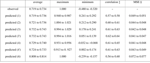
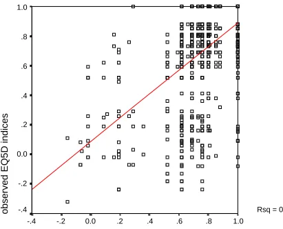
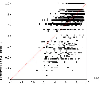
3.2. Goodness of fit
Goodness of fit is summarised in Table 2. While the OLS models (1) to (4') do better in terms
of average predicted EQ5D compared to model (6), these models struggle to produce EQ5D
indices that are negative. The improvement in moving down the list of OLS models can be
the observed indices have a correlation coefficient ranging from 0.56 (model 6, dataset R123)
to 0.65 (model 4, dataset R1). Models (1) and (6) tend to be worse while models (3') and (4)
perform better. In terms of prediction error, there is little difference between the OLS models,
but models (3') and (4) perform slightly better than the others. Model (6) performs markedly
worse compared to the OLS models. Figure 1 is a scatter plot between the observed and
predicted EQ5D indices with model (6), using dataset R1, where the straight line drawn is the
trend line through the plots. The figure illustrates the low concentration of the predicted
EQ5D indices and their biased structure. Figure 2 illustrates the case of model (4), using
dataset R1. Here, a higher concentration of the predicted values is observed, and the trend
line coincides with the 45° diagonal, representing the unbiased nature of the prediction.
3.3. Robustness
For the OLS models, increase in error by going from within sample predictions to out of
sample predictions is very small (less than 0.003), and the variation across the three trials is
smaller (less than 0.002), thus implying the robustness of the models. Dataset R1 tends to
have slightly smaller errors than R23 and R123. Again, model (6) does not perform well,
suggesting that this is less robust than the others. Examination of scatter plots (not shown)
suggests that the patterns of prediction and of errors are roughly the same between the split
samples and the corresponding whole samples.
This section will address three issues. The first is, given the results, which model should be
recommended when EQ5D indices are to be estimated based on AQLQ data. The second is
an exploration of the relationship between the two instruments given the results above. The
last is the implications for mapping non-preference-based measures onto a preference-based
one.
4.1. Recommended model
In terms of goodness of fit, models (3') and (4) do best. We favour model (4) for two reasons.
Firstly, model (3') involves additional variables to model (3), not all of which have the
expected sign or significance level, while model (4) performs only marginally worse.
Secondly, model (3') requires the additional assumption (a) that the AQLQ item levels satisfy
the interval property (see section 1.1 above). The regression coefficients of model (4)
demonstrate that this assumption does not hold. While model (4) involves some inconsistent
coefficients, accounting for these (as in model 4') does not lead to improvements in goodness
of fit. Further, given that the number of items involved is not small, model (3), with fewer
independent variables, may be seen as more practical. It will be advisable therefore to use
model (4) for the main prediction, but to employ models (3), (4') and/or (3') as sensitivity
analyses. When the AQLQ version in question is the original individualised version, then the
coefficients based on R1 is recommended. When the standardised version is used, there is
little to choose between the coefficients based on R23 and those based on R123.
This sub-section will discuss the relationship between the descriptive content of EQ5D and
AQLQ. If the relationship between EQ5D and AQLQ is stable, one would expect the same
set of independent variables to be selected for model (4) across the three datasets. If on the
other hand, there was no stable relationship, then the particular AQLQ items selected for one
dataset may not apply to another dataset. Ignoring AQLQ items 1 to 5 (since they are not
directly comparable between datasets R1 and R23 and were dropped from dataset R123),
there are three AQLQ items with β coefficients that demonstrate the expected sign and good
significance level across all three datasets: 6, 25, and 31. Six more items (16, 27, 28, 29, 30,
and 32) are selected in two datasets, and there is only one item that is selected in one dataset
alone (14). All this seems to indicate that the set of AQLQ items that are selected for model
(4) is reasonably stable across the three datasets, implying a stable relationship across the two
instruments.
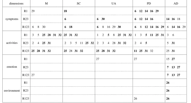
Another way in which to explore this matter is to look at the results of model (5). While the
results of this model are not expected to yield an algorithm with which to estimate EQ5D
indices based on AQLQ data, it offers empirical information on the relationship between
EQ5D dimensions and AQLQ items. Table 3 shows those AQLQ items where the association
between the item and an EQ5D dimension is in the expected direction (β > 0) and p < 0.1, and
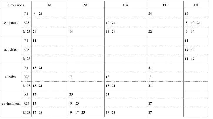
Table 4 shows items with the reverse association (β < 0) and p < 0.1. The AQLQ items are
grouped by their domains. From the first table, it can be seen that: the AQLQ items from the
activities domain affect all EQ5D dimensions; the AQLQ items in the symptoms domain
affect the EQ5D pain/discomfort and anxiety/depression dimensions most; and the emotions
However, Table 4 illustrates that for a number of AQLQ items the association with EQ5D
dimensions is opposite to that expected, and that some of them are also persistent across the
three datasets. Again, this suggests a stable relationship (albeit not in the expected direction)
between the two instruments. It is not clear why AQLQ items such as 10 or 24, which are
straightforward questions on asthma symptoms (“did you experience a wheeze in your chest?”
“were you woken at night by your asthma?”), should result in this unexpected association.
However, items 9, 17, and 23 merit some discussion. These items are worded as “did you
experience asthma symptoms as a result of being exposed to cigarette smoke? / as a result of
being exposed to dust? / as a result of the weather or air pollution outside?”. The reason for
the reverse association between EQ5D and these items may be that, if the patient (for
whatever reason) has problems with mobility, self care, or usual activities, and thus does not
go out, then this individual will not be exposed to cigarette smoke, outdoor dust or air
pollution, and therefore as a result will not experience asthma symptoms in this way. In other
words, better AQLQ levels can be associated with worse EQ5D levels. The only other AQLQ
item worded similarly (item 26) has no association (expected or reverse) with EQ5D. This
interpretation, if correct, throws light on the different conceptualisations of quality of life
behind the two instruments. While on the one hand EQ5D targets problems in different
dimensions of health regardless of their cause, on the other hand AQLQ looks into not only
the experience of asthma symptoms but different causes and triggers for the symptoms, and
how potential or anticipated symptoms affect patient behaviour. This relates to assumption
(c').
This study has shown that it is possible to estimate a robust relationship between EQ5D
indices with AQLQ. Thus, it is not impossible to obtain changes in quality of life in terms of
preference-based single indices in a clinical trial where no direct observation is available.
However, given that non-based condition specific instruments and
preference-based generic instruments are designed to measure different concepts of quality of life, one
cannot substitute completely for the other, and mapping from one to the other is a second best
strategy.
Given the large error associated with the prediction of EQ5D indices, none of these
coefficients can be used to predict EQ5D indices of an individual patient. This study can be
understood as a modelling exercise, where the observations are not systematically assigned to
respondents, but are naturalistically determined by respondents’ self-reported health. The
obvious shortcoming compared to a more experimental setting is the skewed distribution of
health states for which data are available. (This does not mean that the original data comes
from a biased sample, but simply reflects the natural pattern of variability and skew in health
status in the population of interest.) In the context of a modelling study, the ideal distribution
of states would be evenly spread, with a good number of observations for each state: but the
available information only covers an extremely small portion of all the possible AQLQ health
states, and most respondents give the only available observation regarding the particular state
they are in. This has two drawbacks: firstly, there are simply not enough data on the worst
levels; and secondly, the data fed into the model is not rich enough to say what is the average
EQ5D index of a group of patients with a given AQLQ response, because there are only a
There may be those who expect this kind of approach to replace the need to include
preference-based instruments in a clinical trial altogether: if EQ5D indices can be predicted
from AQLQ, or from any other instrument that is more widely accepted in the medical
community, why bother arguing with medical colleagues over the necessity of burdening the
patients with yet another instrument that provides information that could be derived through
the instruments already included? Our findings, however, suggest that the derivation of
preference values is only a poor second best: while the functional relationships are stable, the
predictions have wide margin of error and the method is totally inappropriate for predicting
EQ5D indices at the individual level. The costs of taking this approach (although not exactly
quantified) are no doubt much larger than the marginal cost of including an EQ5D or other
References
1. Juniper EF, Guyatt GH, Ferrie PJ, Griffith LE. Measuring quality of life in asthma.
American Review of Respiratory Disease 1993;147:832-838.
2. Juniper EF, Buist AS, Cox FM, Ferrie PJ, King DR. Validation of a standardized version
of the Asthma Quality of Life Questionnaire. Chest 1999;115(5):1265-1270.
3. Brooks R for the EuroQol Group. EuroQol: The current state of play. Health Policy
1996;37:53-72.
4. Dolan P. Modelling valuation for Euroqol health states. Medical Care 1997;35:351-363.
5. The MVH Group. The Measurement and Valuation of Health: Final Report on the
Modelling of Valuation Tariffs: Centre for Health Economics, University of York; 1995.
6. Revicki DA, Leicy NK, Brennan-Diemer F, Sorensen S, Togias A. Integrating patient
preferences into health outcomes assessment: The multiattribute asthma symptom utility
index. Chest 1998;114:998-1007.
7. McKenzie L, Carins J, Osman L. Symptom-based outcome measures for asthma: The use
of discrete choice methods to assess patient preferences. Health Policy 2001;57:193-204.
8. Chancellor J, Coyle D, Drummond M. Constructing health state preference values from
descriptive quality of life outcomes: Mission impossible? Quality of Life Research
1997;6:159-168.
9. Brazier JE, Usherwood TP, Harper R, Jones NMB, Thomas K. Deriving a preference
based single index measure for health from the SF-36. Journal of Clinical Epidemeology
1998;51(11):1115-1129.
10. Brazier J, Roberts J, Deverill M. The estimation of a utility based algorithm from the
11. Coast J. Reprocessing data to form QALYs. British Medical Journal
1992;305(6845):87-90.
12. Eccles M, Grimshaw J, Steen N, Parkin D, Purves I, McColl E, et al. The design and
analysis of a randomized controlled trial to evaluate computerized decision support in
Table 1: Summary of regression models
model dependent variable D/C † independent variables D/C †
(1) (2) (3) (3') (4) (4') (5) (6) EQ5D index EQ5D index EQ5D index EQ5D index EQ5D index EQ5D index EQ5D dimension-level EQ5D dimension-level C C C C C C C D
AQLQ overall score
all AQLQ domain scores
all AQLQ item levels
all AQLQ item levels + interactions
selected AQLQ item levels
further selected AQLQ item levels
all AQLQ item levels
selected AQLQ item levels
Table 2: Summary of regression results across the three datasets
average maximum minimum correlation ‡ MSE §
observed predicted (1) predicted (2) predicted (3) predicted (3') predicted (4) predicted (4') predicted (6)
0.719 to 0.734
0.719 to 0.736
0.721 to 0.736
0.732 to 0.743
0.732 to 0.743
0.729 to 0.740
0.724 to 0.733
0.808 to 0.814
1.000
0.940 to 0.987
1.004 to 1.021
0.994 to 1.029
0.994 to 1.016
0.931 to 0.956
0.913 to 0. 927
1.000
-0.480 to -0.320
0.241 to 0.292
0.212 to 0.290
0.178 to 0.241
0.051 to 0.139
-0.032 to +0.068
0.002 to 0.174
-0.239 to -0.157
-
0.57 to 0.58
0.60 to 0.61
0.61 to 0.63
0.62 to 0.64
0.61 to 0.65
0.61 to 0.63
0.56 to 0.60
-
0.049 to 0.051
0.044 to 0.048
0.042 to 0.048
0.041 to 0.047
0.041 to 0.048
0.043 to 0.049
0.072 to 0.077
† Predicted EQ5D indices cannot be calculated for model (5).
‡ Range of Pearson’s correlation coefficient between observed and predicted EQ5D indices, across the three datasets.
Table 3: EQ5D dimensions and AQLQ items: AQLQ items with the expected association in model (5) (p<0.1, bold if across two datasets)
dimensions M SC UA PD AD
R1 29 18 6 12 14 16 29
R23 6 6 30 6 12 14 16 14 16 18
symptoms
R123 6 8 30 6 18 6 8 16 29 30 6 8 12 14 16 29 6 14 16 29
R1 3 5 25 28 31 32 25 31 32 1 2 5 8 25 31 32 1 3 5 11 25 31 3 6
R23 2 4 25 31 2 3 5 11 25 32 2 3 4 28 31 32 2 4 5 5 31
activities
R123 25 28 31 32 25 28 31 32 25 28 31 32 11 25 31 32 25 31
R1 27 27 15 27
R23 7 13 27
emotion
R123 27 7 13 27
R1 26
R23 26
environment
Table 4: EQ5D dimensions and AQLQ items: AQLQ items with the reverse association in model (5) (p<0.1, bold if across two datasets)
dimensions M SC UA PD AD
R1 6 24 24 10
R23 10 24 8 10 24
symptoms
R123 24 14 14 24 22 9 10
R1 11 11
R23 1 19 32
activities
R123 11 19
R1 13 21 21
R23 7 15 7
emotion
R123 13 21 15 21 21
R1 17 23 23
R23 17 9 23 17
environment
Figure 1: The performance of model (6) dataset R1
predicted EQ5D indices: model (6) dataset R1
1.0 .8
.6 .4
.2 0.0
-.2 -.4
observed EQ5D indices
1.0
.8
.6
.4
.2
0.0
-.2
Figure 2: The performance of model (4) dataset R1
predicted EQ5D indices: model (4) dataset R1
1.0 .8
.6 .4
.2 0.0
-.2 -.4
observed EQ5D indices
1.0
.8
.6
.4
.2
0.0
-.2
Appendix 1: The EQ5D instrument
Mobility
No problems in walking about
Some problems in walking about
Confined to bed
Self-Care
No problems with self-care
Some problems washing or dressing oneself
Unable to wash or dress oneself
Usual Activities (e.g. work, study, housework, family or leisure activities)
No problems with performing one’s usual activities
Some problems with performing one’s usual activities
Unable to perform one’s usual activities
Pain/Discomfort
No pain or discomfort
Moderate pain or discomfort
Extreme pain or discomfort
Anxiety/Depression
Not anxious or depressed
Moderately anxious or depressed
Extremely anxious or depressed
some problems in walking about,
no problems washing and dressing oneself,
some problems with performing one’s usual activities,
extreme pain or discomfort, and
moderately anxious or depressed.
Appendix 2: The Asthma Quality of Life Questionnaire (the original individualised version)
[Each of the following questions is followed by a 7-point scale with appropriate labels to do with degrees of
limitation, or frequency of the problem, etc. The smaller the level, the more severe. Items are marked here
with S (symptoms), A (activities), Em (emotions), En (environment), to represent the 4 domains.]
[A list of 26 activities such as bicycling, dancing, carrying out DIY, doing housework, gardening etc. is first
given, and respondents are asked to write out “the 5 most important activities in which you have been
limited by your asthma during the last 2 weeks” on 5 spaces linked to Q1 to Q5.]
A 1-5 How limited have you been during the last 2 weeks in these activities?
S 6 How much discomfort or distress have you felt over the last 2 weeks as a result of chest tightness?
In general, how much of the time during the last 2 weeks did you:
Em 7 feel concerned about having asthma?
S 8 feel short of breath as a result of your asthma?
En 9 experience asthma symptoms as a result of being exposed to cigarette smoke?
S 10 experience a wheeze in your chest?
A 11 feel you had to avoid a situation or environment because of cigarette smoke?
S 12 How much discomfort or distress have you felt over the last 2 weeks as a result of coughing?
In general, how much of the time during the last 2 weeks did you:
Em 13 feel frustrated as a result of your asthma?
S 14 experience a feeling of chest heaviness?
Em 15 feel concerned about the need to use medication for your asthma?
S 16 feel the need to clear your throat?
A 19 feel you had to avoid a situation or environment because of dust?
S 20 wake up in the morning with asthma symptoms?
Em 21 feel afraid of not having your asthma medication available?
S 22 feel bothered by heavy breathing?
En 23 experience asthma symptoms as a result of the weather or air pollution outside?
S 24 were you woken at night by your asthma?
A 25 avoid or limit going outside because of the weather or air pollution?
En 26 experience asthma symptoms as a result of being exposed to strong smells or perfume?
Em 27 feel afraid of getting out of breath?
A 28 feel you had to avoid a situation or environment because of strong smells or perfume?
S 29 has your asthma interfered with getting a good night’s sleep?
S 30 have a feeling of fighting for air?
How limited have you been during the past 2 weeks?
A 31 Think of the overall range of activities that you would have liked to have done during the last 2
weeks. How much has your range of activities been limited by your asthma?
A 32 Overall, among all the activities that you have done during the past 2 weeks, how limited have you
been by your asthma?
[In the standardised version, the first five items (all of them S) are changed to:]
How limited have you been during the last 2 weeks in these activities as a result of your asthma?
1 strenuous activities (such as hurrying, exercising, running up stairs, sports)
2 moderate activities (such as walking, housework, gardening, shopping, climbing stairs)
3 social activities (such as talking, playing with pets/children, visiting friends/relatives)
4 work related activities* (tasks you have to do at work)
5 sleeping