Determination of multi-component flow process parameters based on electrical capacitance tomography data using artificial neural networks

This is a repository copy of Determination of multi-component flow process parameters based on electrical capacitance tomography data using artificial neural networks .

White Rose Research Online URL for this paper: http://eprints.whiterose.ac.uk/743/

Article:

Mohamad-Saleh, J. and Hoyle, B.S. (2002) Determination of multi-component flow process parameters based on electrical capacitance tomography data using artificial neural networks. Measurement Science and Technology, 13 (12). pp. 1815-1821. ISSN 1361-6501

https://doi.org/10.1088/0957-0233/13/12/303

[email protected] https://eprints.whiterose.ac.uk/ Reuse

See Attached

Takedown

If you consider content in White Rose Research Online to be in breach of UK law, please notify us by

White Rose Consortium ePrints Repository

http://eprints.whiterose.ac.uk/

This is an author produced version of a paper published in Measurement Science and

Technology. This paper has been peer-reviewed but does not include the final

publisher proof-corrections or journal pagination.

White Rose Repository URL for this paper: http://eprints.whiterose.ac.uk/archive/00000743/

Citation for the published paper

Hoyle, B.S. and Jia, X. and Podd, F.J.W. and Schlaberg, H.I. and Wang, M. and West, R.M. and Williams, R.A. and York, T.A. (2001) Design and application of a multi-modal

process tomography system. Measurement Science and Technology, 12 (8). pp.

1157-1165.

Citation for this paper

Hoyle, B.S. and Jia, X. and Podd, F.J.W. and Schlaberg, H.I. and Wang, M. and West, R.M. and Williams, R.A. and York, T.A. (2001) Design and application of a multi-modal

process tomography system. Author manuscript available at:

http://eprints.whiterose.ac.uk/archive/00000743/ [Accessed: date]. Published in final edited form as:

Hoyle, B.S. and Jia, X. and Podd, F.J.W. and Schlaberg, H.I. and Wang, M. and West, R.M. and Williams, R.A. and York, T.A. (2001) Design and application of a multi-modal

process tomography system. Measurement Science and Technology, 12 (8). pp.

1157-1165.

Determination of multi-component flow process parameters

based on electrical capacitance tomography data using

artificial neural networks

J Mohamad-Saleh and B S Hoyle

Institute of Integrated Information Systems, School of Electronic and Electrical Engineering, University of Leeds, Leeds LS2 9JT, UK.

E-mail: [email protected]

Abstract. Artificial neural networks have been used to investigate their capabilities at

estimating key parameters for the characterisation of flow processes, based on electrical capacitance-sensed tomographic (ECT) data. The estimations of the parameters are done directly, without recourse to tomographic images. The parameters of interest include component height and interface orientation of two-component flows, and two-component fractions of two-two-component and three-two-component flows. Separate multi-layer perceptron networks were trained with patterns consisting of pairs of simulated ECT data and the corresponding component heights, interface orientations and component fractions. The networks were then tested with patterns consisting of unlearned simulated ECT data of various flows and, with real ECT data of gas-water flows. The neural systems provided estimations having mean absolute errors of less than 1% for oil and water heights and fractions; and less than 10° for interface orientations. When tested with real plant ECT data, the mean absolute errors were less than 4% for water height, less than 15° for gas-water interface orientation and less than 3% for water fraction, respectively. The results demonstrate the feasibility of the application of artificial neural networks for flow process parameter estimations based upon tomography data.

Keywords: electrical capacitance tomography, neural networks, process

interpretation, multi-component flows.

1. Introduction

The application of electrical capacitance tomography (ECT) systems for quantitative measurement purposes in a range of processes is well established due to its non-invasive and non-hazardous properties [1-4]. Systems have mainly centred upon the approximate solution of the inverse problem of tomographic image

reconstruction. In many laboratory-targeted demonstrations, the resulting images of the process in operation are the end-point. For real plant and process use, however, interpretations are required to relate the internal process information to typical process reference frames.

The Linear Back-Projection (LBP) algorithm [5], the most commonly used image reconstruction algorithm for ECT, is computationally simple, but suffers from the soft-field effect, smearing sharp transitions between materials of differing

More sophisticated reconstruction methods have been proposed to reduce or eliminate the smearing effects in reconstructed images. Examples are the iterative LBP algorithm [7], the algebraic reconstruction algorithm [8] and the model-based reconstruction algorithm [9-10]. Nevertheless, these algorithms are not normally preferred, usually because the reconstruction speed is too slow relative to the real-time needs of the process, or because the gains in image quality are marginal. Although the problem of reconstruction speed is diminishing as processing speeds increase, the use of these algorithms will not be preferable until a satisfactory real-time

reconstruction speed is achieved.

Research in capacitance-sensed tomographic image reconstruction has also focussed upon the neural computation approach. A number of pilot investigations have developed artificial neural networks (ANNs) [11-12] for image reconstruction [13-19]. The approach has been shown to produce improved reconstructed images, and thus more accurate parameter estimations than the conventional methods.

In many cases, estimation of key process parameters is of more interest than the estimation of images. For example, in flow processes, characterisation is likely to be based upon component fraction and interface state. Hence some research effort has been channelled toward direct methods of process interpretation that do not include image reconstruction. In this role such solutions are expected to be more efficient and cost effective than conventional techniques.

A number of direct techniques, based on electrical capacitance tomography, have incorporated the use of ANNs for flow process parameter estimation. Duggan and York investigated a RAM-based neural network model to directly estimate the component fraction of oil in gas-oil flows [13-14]. Williams and York also used the RAM-based neural network, implemented in specialised hardware, to also determine the component fraction of oil in gas-oil flows [18]. Initial investigations by Mohamad Saleh et al. have revealed the capability of multi-layer feed-forward neural networks in direct component fraction estimations of oil in gas-oil flows, water in gas-water flows and, and oil and water in gas-oil-water flows [20]. This paper summarises key results to offer a comprehensive view and extend these in detail to provide fuller dynamic model estimation such as interface height and orientation. The composite data is intended to offer comprehensive support for multi-component flow studies.

The robustness demonstrated by ANNs, in direct flow component fraction estimation, has motivated the use of a similar approach for the estimation of other flow parameters. In this paper we discuss the use of ANNs for direct estimations of oil height in gas-oil flows, water height in gas-water flows, gas-oil interface

orientation, and gas-water interface orientation. This offers new possibilities for component fraction estimation in dynamically evolving flows. Novel techniques are presented for component fraction estimation of two-component as well as three-component flows using the neural network approach based on ECT data. The results obtained reveal the robustness of the ANN system for direct component fraction estimation of two-component (typically two-phase) and three-component flows (for example comprising oil, water and gas; sometimes called three-phase flows). Figure 1 illustrates the flow parameters of interest. As shown the height is the depth of the liquid component normal to its nominal interface. For high flow rates the interface can be expected to be very mobile.

2. Development of the estimation system

Three stages are involved in the development of the proposed system; (i) ECT dataset collection and pre-processing, (ii) ANN training and (iii) ANN testing, or verification.

Simulated ECT data was used for a number of reasons. Actual plant data for complex flow regimes is extremely difficult to generate in the reliable and repeatable manner required. Also a specific plant and ECT system will inevitably include some asymmetry and specific noise. This may result in the over-training of the ANN to characteristics of the specific plant. In contrast the aim in this work was a generic training process, independent of a particular plant. The use of simulation data also provides much more variety than could have been obtained with the practical

constraints of laboratory-based exercise. Simulated ECT data were obtained using a simulator, developed at the University of Leeds, based on a two-dimensional finite-element method [21].

As shown in figure 2, the simulator takes the relative permittivity of each component, together with the flow geometry involved in the flow process, to calculate the corresponding raw ECT measurements. At the same time, the actual flow process parameters (component heights, interface orientation and component fractions) of materials for the particular flow process are calculated.

Raw ECT measurements are passed to a pre-processor, which transforms the data into orthogonal components, using the Principal Component Analysis (PCA) method [22]. For the purpose of this investigation, raw ECT measurements

corresponding to various flow regimes including stratified, annular and bubble flow were collected. In addition to simulated data, real plant ECT data were also obtained through colleagues in the Virtual Centre for Industrial Process Tomography (VCIPT).

Figure 2. Schematic diagram of simulation and pre-processing of ECT data.

As illustrated in figure 3, training patterns, consisting of pairs of uncorrelated ECT data obtained from the orthogonal dataset and the corresponding flow parameter value, are used to train an MLP. The training procedure was based on a variant of the Back Propagation algorithm, known as the Bayesian Regularisation algorithm [23-24]. During each training cycle, the uncorrelated ECT measurements, as the inputs to the MLP, are used together with the MLP’s weight values to obtain an estimated output parameter value. The difference between the MLP-estimated and the actual flow parameter values is back-propagated into the MLP to update the network’s weights for use in the next training cycle. The process is repeated until the MLP has reached a satisfactory performance.

Figure 3. Schematic diagram of MLP training procedure.

Eight separate MLPs were trained for the different flow process parameter estimation tasks tabulated below. Four of the MLPs noted below relate to component fraction estimation, and four to interface height and orientation.

MLP_6 Water fraction estimation of gas-water flows MLP_7 Oil fraction estimation of gas-oil-water flows MLP_8 Water fraction estimation of gas-oil-water flows

Table 1. MLP flow parameter estimation tasks

Once the training processes were completed, the MLPs were tested with a set of (unlearnt) simulated ECT measurements. The ECT measurements were first pre-processed, using the PCA technique, before being passed to the developed MLPs, designed to estimate the flow process parameter values. The performances of the MLPs were measured in terms of their mean absolute test errors, based on the set of test patterns used.

Those MLPs that were trained with association to gas-water flows (MLP_3, MLP_4 and MLP_6) were also tested with sets of real plant ECT measurements of gas-water flows. These include measurements based on static and dynamic flows.

The static tests were carried out on a small capped pipe section equipped with Perspex end plates with calibration scales. This could be filled to given level to provide a physical simulation of a stratified flow. Physical simulations of annular and bubbles flows were provided by using tubes that could be inserted at a given position in the cross-section.

The sensor electrodes in this static physical simulation did not correspond exactly to the simulation parameters used for training. Since these differences can be expected to appear only as subtle changes in the electric field, it is complex to

quantify them, except through the trial. A background aim of this investigation was to test the extent to which the ‘generic’ simulation-trained network is useful in

interpreting data from the same class of ECT sensor, even where the detailed

parameters of electrode arrangements differ. Here the term “same class” implies the same number of electrodes, and the same topology. For example, 12-electrode and circular topology ECT sensors were used in all tests reviewed in this paper. Thus the static trial sensor provides an opportunity to explore this capability, albeit in a

qualitative manner in this work.

The dynamic tests were carried out on a flow loop and restricted to gas/water flow. Once again the available sensor did not have exactly the same physical

arrangement as either, the simulation parameters, or, the static physical simulation sensor, providing a further opportunity to test the generic interpretation capability.

In this case, however, independent instrumentation was not available to measure the actual flow parameters. Although a video camera was installed on the experimental rig, it was positioned on the side of the pipe. Hence, images

reconstructed by the MLPs could only be compared to the actual video images at the corresponding time reference for a general verification of the MLPs’ performance. These tests are intended to illustrate the system in actual dynamic use rather than building upon the quantitative aspects of the investigation.

3. Results and discussion

3.1 Simulated ECT data

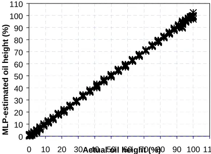
directly and accurately determine oil heights from gas-oil flows without recourse to reconstructed images.

Figure 4. MLP_1 estimations of oil height with reference to actual height

values of gas-oil flows.

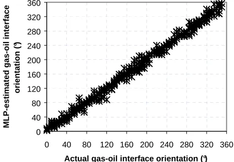
Figure 5 shows the results of gas-oil interface orientations, as estimated by MLP_2, with reference to the actual interface orientation values. It can be seen that the MLP’s estimations are quite close to the actual interface orientation values. The linear regression coefficient of the plot is again 1. This demonstrates the feasibility of the MLP estimator for direct interface orientation estimations from gas-oil flows.

Figure 5. MLP_2 estimations of gas-oil interface orientation with reference to

actual orientations.

MLP_3’s estimations of water heights in comparison to the actual water height values are shown in figure 6. The regression coefficient of the plots is 1,

demonstrating the capability of the MLP for estimating water heights from gas-water flows.

Figure 6. MLP_3 estimations of water height with reference to actual height

values of gas-water flows.

Figure 7 shows the results of gas-water interface orientations, as estimated by MLP_4, versus the actual interface orientations. The regression coefficient of the plot is 0.98. The smallest and largest estimation errors are 0.01° and 98°, respectively. Most of the largest errors occur when estimating the interface orientation of annular flows, which have the value of 1 (i.e. corresponding to 360°) for annular flows, bubble flows and for the pipe when full of water. This is because MLP_4 has

difficulty in mapping different trends of capacitance measurements to the same output value. Despite this limitation, the mean absolute test error produced is rather small.

For component fraction estimation, MLP_5 produced a mean absolute error of 0.32%±0.01% for oil fraction estimation, from gas-oil flows, when tested with a set of simulated test patterns.

MLP_6 produced a mean absolute test error of about 0.7%±0.6% for water fraction estimations from gas-water flows.

Figure 7. MLP_4 estimations of gas-water interface orientation with reference

to actual orientations.

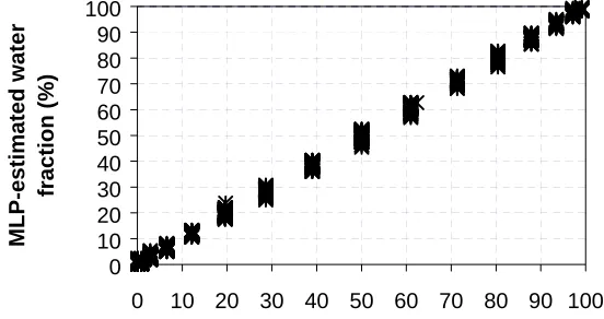
Figure 8 and figure 9 present the results of the oil and water fractions from gas-oil-water flows as estimated by MLP_7 and MLP_8, respectively, with reference to the actual fraction values. The mean absolute errors with their standard deviations for oil and water fraction estimations are 0.85%±0.7% and 0.72%±0.6%, respectively. The results revealed that it was easier for an MLP to estimate water fractions than oil fractions, from gas-oil-water flows. This is because the raw capacitance

associated to water than to the data associated to oil. Even though the errors produced for oil fraction estimations are larger than for water, they are rather small, suggesting that MLPs are good at estimating individual material fraction values from three-component flows. The results demonstrate that an ECT system, incorporating the ANN, can be a useful means of extracting three-component flow parameters.

Figure 8. MLP_7 estimations of oil fractions from various regimes of

gas-oil-water flows in comparison to actual fraction values.

Figure 9. MLP_8 estimations of water fractions from various regimes of

gas-oil-water flows in comparison to actual fraction values.

Further analysis of the results reveals that the MLPs estimate parameters of stratified flows more accurately than bubble and annular flows. This is due to the larger number of stratified flow patterns used for network training compared to bubble and annular flow patterns. The fact that fewer bubble and annular flow patterns than stratified are used in the training data set is because of the limited number of patterns that can be generated from these regimes.

3.2 Real plant ECT data for static gas-water flows

These trials were carried out on data obtained using the capped pipe section and ECT sensor described in Section 2.

Figure 10 shows the MLP_3 estimations with reference to the actual water heights for different flow regimes. It can be seen in the figure that the estimation of water height for a full pipe (one) offers good accuracy. The estimation of water height for an empty (zero) pipe also offers good accuracy (not shown in the figure). This is because MLP_3 has been trained with capacitance values corresponding to these flow patterns. The mean absolute test errors produced by MLP_3 for water height estimations are 2%±0.2%, 4%±0.14% and 5%±0.14% for stratified, bubble and annular flow patterns, respectively.

Figure 10. MLP_3 estimations of water heights in comparison to actual height

values for patterns of stratified, bubble and annular flow regimes.

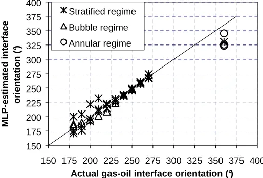
The results of gas-water interface orientation estimations produced by MLP_4 are shown graphically in figure 11. The mean values of absolute error for the

estimations are 7.3°, 4.3° and 28.5° with variance values of 0.2°, 0.03° and 0.4° for stratified, bubble and annular flows, respectively. Most of the interface orientation estimation errors for stratified and bubble flow patterns are smaller than those of annular flows. The largest error is about 36.5°, produced when estimating the interface orientation of an annular flow. The large mean error, in the interface orientation estimations of annular flows, is likely to be due to the network confusion that arises because the same interface orientation value (of one) is used for a pipe that is full of water, and for all annular flow patterns during network training. Another factor that contributes to the larger estimation errors in annular flows is the fact that only limited number of annular flow patterns can be generated and used to train the MLP estimators, in comparison to stratified and bubble flow patterns.

Figure 11. MLP_4 estimations of gas-oil interface orientations with reference

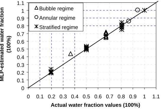
Figure 12 shows the results of MLP_6 estimation of water fractions from gas-water flows with reference to the actual fraction values for stratified, bubble and annular flow regimes. It can be seen that most of MLP_6 estimations, of water fraction from stratified flows, correspond well to the actual values. The mean absolute error for the estimations is about 1.3%, with a variance of 0.02% for stratified flows; 3.6% with a variance of 0.05% for bubble flows; and 2.5% with a variance of 0.1% for annular flows. These results are similar to those for the cases of water height and gas-water interface orientation estimation; in that they show that the MLP is better at estimating water fractions of stratified flows, than bubble and annular flows. The explanation of these findings is the same as that of water height and interface orientation estimations.

Figure 12. MLP_6 estimations of water fractions with reference to actual water

fraction values for patterns of stratified, bubble and annular flow regimes.

For all the three flow parameter estimations, the MLP estimation errors are larger when tested with the real plant ECT data reviewed here, than with the simulation reviewed in section 3.1 above.

This is likely to be due partly to specific electronic noise present in ECT measurements from a particular sensor. Also, as noted in Section 2, the ECT sensor does not have the same parameters as the simulation used for training, although assessing the difference will be complex as this must be studied in terms of the effect on the electric field generated for a particular object configuration. Hence the relative performance does provide an indication of the value of the simulation training in ‘generic’ interpretation, for a given class of ECT sensor. Of course the MLP performance could be expected to have been improved had it been trained with the specific noisy data-sets from the actual ECT sensor.

3.3 Real plant ECT data for dynamic gas–water flows

These trials were carried out on data obtained using the flow loop and ECT sensor described in section 2.

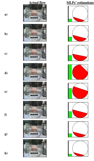
The images in figure 13 show some of the results for flow parameter

estimations based on these dynamic gas-water flows. The images on the left are video clips of the gas-water flows at a known time synchronised with data collection. This figure is intended to be qualitative only, its major aspect being in the interpreted data of the right hand column.

Figure 13. A comparison between the actual flow and the MLPs’ estimations of water

height, gas-water orientation and water fraction of dynamic gas-water flows.

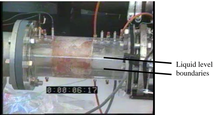
Figure 14 provides an enlarged view of one flow condition, frame (f), to illustrate how the estimated level can be verified from the synchronised video frame. Lines have been added to this figure 14 to highlight the stratified level.

Figure 14. Enlarged view of one frame (f) to show how estimates of stratified level

The right column shows cross-sectional images of the pipe, generated simply from MLPs’ estimations of water height and gas-water interface orientation. The vertical calibration line on the left of each image is a reference for the water fraction. The bar column shown indicates the water fraction as estimated by MLP_6.

The generated images of figure 13(a), (b) and (c) show increasing water level, and these agree with the corresponding video frames.

A plug of water rushing through the pipe is depicted in the video frame of figure 13(d). The corresponding generated image (d) shows an increase in the water level and fraction, and a sudden change in the interface orientation value. The video frames of Figure 13(e) to (h) show decreasing water level, and these agree with the generated images.

The generated images demonstrate that an ANN estimation system is able to give sensible flow parameter estimation values for dynamic flows.

As in the case of the static trials reviewed in Section 3.2, the system performs well in this ‘generic’ interpretation mode; where training has not employed the actual data from the ECT sensor, and which differs from the parameters used in the training simulation. Typically errors are increased by about 1%. As above, it is likely that performance would be improved if such a system specific training were employed.

The direct estimation of flow parameters for 1000 gas-water flow patterns takes an average of about 44s on a 64MHz stand-alone PC when computed in sequence. This means that the software ANN algorithm takes an average of about 44ms to estimate the component height, interface orientation and component fraction of each flow pattern (corresponding to about 1ms on a current 2GHz computer assuming a linear speedup). The use of dedicated neural computing hardware could provide parallel execution in the ANN and reduce the processing time further.

4. Conclusions

The research concentrated on the development and application of ANN methods and investigated its suitability at estimating process flow parameters: component height, interface orientation, and component fraction. The experimental results demonstrated the feasibility of applying ANN methods for flow parameter estimation without recourse to image reconstruction. The developed ANN estimation system has been robust at determining component heights and interface orientations of two-component flows and component fractions of two-component and

three-component flows. Among the advantages offered by the system are fast response, direct process flow parameter estimations, tolerance to instrumentation noise and capability in dealing with multi-component flows. The system also demonstrates its ‘generic’ interpretation capability, where the actual ECT sensor is of the same class but its measurement data has not been used in ANN training.

References

[1] Beck M S, Byars M, Dyakowski T, Waterfall R, He R, Wang S J and Yang W Q 1997 Principles and industrial applications of electrical capacitance

tomography Measurement + Control 30 197-200

[2] Reinecke N and Mewes D 1996 Recent developments and industrial/research applications of capacitance tomography Meas. Sci. Technol. 7 233-246 [3] Williams, R A and Beck M S (eds) 1995 Process Tomography: Principles,

[4] Yang W Q, Beck M S and Byars M 1995 Electrical capacitance tomography – from design to applications Measurement + Control 28 261-266

[5] Xie C G, Plaskowski A and Beck M S 1989 8-electrode capacitance system for two-component flow identification:Tomographic flow imaging IEE

Proceedings 136 173-183

[6] Isaksen Ø 1996 A review of reconstruction techniques for capacitance tomography Meas. Sci. Technol. 7 325-337

[7] Chen Q, Hoyle B S and Strangeways H J 1992 Electrical field interaction and an enhanced reconstruction algorithm in capacitance process tomography Proc.

1st ECAPT Conf. (Manchester 26-29 March 1994) 205-212

[8] Reinecke N and Mewes D 1994 Resolution enhancement for multi-electrode capacitance sensors Reviewed Proc. 3rd ECAPT Conf. (Porto, Portugal, 22-26 March 1994)

[9] Isaksen Ø and Nordtvedt J E 1994 An implicit model based reconstruction algorithm for use with a capacitance tomography system Proc. 3rd ECAPT Conf. (Porto, Portugal, 22-26 March 1994) 215-226

[10] Isaksen Ø and Nordtvedt J E 1993 A new reconstruction algorithm for process tomography Meas. Sci. Technol. 4 1464-1475

[11] Haykin S 1999 Neural Networks: A Comprehensive Foundation London: Macmillan College

[12] Bishop C M 1994 Neural networks and their applications Review of Scientific

Instruments 65 1803-1832

[13] Duggan P M and York T A 1995 Tomographic image reconstruction using RAM-based neural networks Process Tomography--Implementation for

Industrial Processes Proc. 4th ECAPT Conf. (Bergen, Norway, 4-8 April 1995)

411-419

[14] Duggan P M 1997 Application of RAM-based Neural Networks to Electrical

Capacitance Tomography Ph.D. Thesis University of Manchester Institute of

Science and Technology.

[15] Nooralahiyan A Y, Hoyle B S and Bailey N J 1995 Performance of neural network in capacitance-based tomographic process measurement systems

Measurement + Control 28 109-112

[16] Nooralahiyan A Y 1996 Artificial Neural Networks for Image Reconstruction

and Interpretation in Electrical Capacitance Tomography PhD Thesis

University of Leeds

[17] Nooralahiyan A Y and Hoyle B S 1997 Three-component tomographic flow imaging using artificial neural network reconstruction Chemical Engineering

52 2139-2148

[18] Williams P and York T 1999 Hardware implementation of RAM-based neural networks for tomographic data processing IEE Proc.-Comput. Digit. Tech. 146 114-118

[19] Sun T D, Mudde R, Schouten J C, Scarlett B, van den Bleek C M 1999 Image reconstruction of an electrical capacitance tomography system using an artificial neural network Proc. 1st World Congress on Industrial Process Tomography (Buxton, 14-17April 1999) 174-180

[20] Mohamad-Saleh J, Hoyle B S, Podd F J W, Spink D M 2001 Direct process estimation from tomographic data using artificial neural systems SPIE Journal

of Electronic Imaging 10 646-652

International Journal for Computation and Mathematics in Electrical and Electronic Engineering 15 70-84

[22] Jolliffe I T 1986 Principal Components Analysis New York:Springer-Verlag [23] MacKay D J C 1992 Bayesian Interpolation Neural Computation 4 415-447 [24] Forsee F D and Hagan M T 1994 Gauss-Newton approximation to Bayesian

learning Proceedings of the International Joint Conference on Neural

Figures

h

θ

f

Figure 1. Flow process parameters involving component height (h), interface

orientation (θ), and component fraction (f).

Raw ECT dataset

FE Simulation

Component

permittivity _PCA

Corresponding flow process parameters

Ortogonal dataset Flow

geometry

Figure 2. Schematic diagram of simulation and pre-processingof ECT data.

Uncorrelated ECT data

Actual flow parameter value

MLP training

Error

MLP-estimated parameter value

+

Figure 3. Schematic diagram of MLP training procedure.

0 10 20 30 40 50 60 70 80 90 100 110

0 10 20 30 40 50 60 70 80 90 100 110Actual oil height (%)

MLP-e

s

tima

te

d

oil he

ight (%)

Figure 4. MLP_1 estimations of oil height with reference to actual height

0 40 80 120 160 200 240 280 320 360

0 40 80 120 160 200 240 280 320 360 Actual gas-oil interface orientation (°)

MLP

-esti

m

ated gas-oi

l i

n

terface

orientation (°

)

Figure 5. MLP_2 estimations of gas-oil interface orientation with reference to

actual orientations.

0 10 20 30 40 50 60 70 80 90 100

0 10 20 30 40 50 60 70 80 90 100 Actual water height (%)

MLP

estimated water heights

(%)

Figure 6. MLP_3 estimations of water height with reference to actual height

0 60 120 180 240 300 360

0 60 120 180 240 300 360

Actual gas-water interface orientation (°)

MLP estim

ated gas-w

a

ter

interface orientation (°

)

Figure 7. MLP_4 estimations of gas-water interface orientation with reference

to actual orientations.

0 10 20 30 40 50 60 70 80 90 100

0 10 20 30 40 50 60 70 80 90 10 0

Actual oil fraction (%)

MLP- estimated oil fraction

(%)

Figure 8. MLP_7 estimations of oil fractions from various regimes of

gas-oil-water flows in comparison to actual fraction values.

0 10 20 30 40 50 60 70 80 90 100

0 10 20 30 40 50 60 70 80 90 100

Actual water fraction (%)

MLP-estimated water

fraction (%)

Figure 9. MLP_8 estimations of water fractions from various regimes of

0.4 0.5 0.6 0.7 0.8 0.9 1 1.1

0.4 0.5 0.6 0.7 0.8 0.9 1 1.1 Actual water height values (100%)

ML

P-estimated

water h

e

ig

h

ts

(100%)

Stratified regime Bubble regime

Annular regime

Figure 10. MLP_3 estimations of water heights in comparison to actual height

values for patterns of stratified, bubble and annular flow regimes.

150 175 200 225 250 275 300 325 350 375 400

150 175 200 225 250 275 300 325 350 375 400 Actual gas-oil interface orientation (°)

ML

P-estimated

in

terface

orie

nta

tion (°

)

Stratified regime

Bubble regime Annular regime

Figure 11. MLP_4 estimations of gas-oil interface orientations with reference

0 0.1 0.2 0.3 0.4 0.5 0.6 0.7 0.8 0.9 1 1.1

0 0.1 0.2 0.3 0.4 0.5 0.6 0.7 0.8 0.9 1 1.1 Actual water fraction values (100%)

ML

P-estimated

w

a

ter fractio

n

(100%)

Bubble regime Annular regime

Stratified regime

Figure 12. MLP_6 estimations of water fractions with reference to actual water

Actual flow MLPs’ estimations

a)

-1.5 -1 -0.5 0 0.5 1 -1 -0.8 -0.6 -0.4 -0.2 0 0.2 0.4 0.6 0.8 1 b)

-1.5 -1 -0.5 0 0.5 1 -1 -0.8 -0.6 -0.4 -0.2 0 0.2 0.4 0.6 0.8 1 c)

-1.5 -1 -0.5 0 0.5 1 -1 -0.8 -0.6 -0.4 -0.2 0 0.2 0.4 0.6 0.8 1 d)

-1.5 -1 -0.5 0 0.5 1 -0.8 -0.6 -0.4 -0.2 0 0.2 0.4 0.6 0.8 1 e)

-1.5 -1 -0.5 0 0.5 1 -1 -0.8 -0.6 -0.4 -0.2 0 0.2 0.4 0.6 0.8 1 f)

-1.5 -1 -0.5 0 0.5 1 -1 -0.8 -0.6 -0.4 -0.2 0 0.2 0.4 0.6 0.8 1 g)

-1.5 -1 -0.5 0 0.5 1 -1 -0.8 -0.6 -0.4 -0.2 0 0.2 0.4 0.6 0.8 1 h)

-1.5 -1 -0.5 0 0.5 1 -1 -0.8 -0.6 -0.4 -0.2 0 0.2 0.4 0.6 0.8 1

Figure 13. A comparison between the actual flow and the MLPs’ estimations of water

Liquid level boundaries

Figure 14. Enlarged view of one frame (f) to show how estimates of stratified level