Modelling time-constrained software development

This is a repository copy of Modelling time-constrained software development. White Rose Research Online URL for this paper:

http://eprints.whiterose.ac.uk/2562/

Monograph:

Powell, A. (2004) Modelling time-constrained software development. Working Paper. Department of Management Studies, University of York , York.

[email protected] https://eprints.whiterose.ac.uk/

Reuse

Items deposited in White Rose Research Online are protected by copyright, with all rights reserved unless indicated otherwise. They may be downloaded and/or printed for private study, or other acts as permitted by national copyright laws. The publisher or other rights holders may allow further reproduction and re-use of the full text version. This is indicated by the licence information on the White Rose Research Online record for the item.

Takedown

If you consider content in White Rose Research Online to be in breach of UK law, please notify us by

promoting access to White Rose research papers

White Rose Research Online

Universities of Leeds, Sheffield and York

http://eprints.whiterose.ac.uk/

White Rose Research Online URL for this paper: http://eprints.whiterose.ac.uk/2562/

Published work

Powell, A. (2004) Modelling time-constrained software development. Working Paper. Department of Management Studies, University of York, York.

University of York

Department of Management Studies

Working Paper No. 4

ISSN Number: 1743-4041

Modelling Time-Constrained Software Development

Dr. Antony Powell

Department of Management Studies, University of York

This paper is circulated for discussion purposes only and its contents should be

Abstract

Commercial pressures on time-to-market often require the development of software in

situations where deadlines are very tight and non-negotiable. This type of development can

be termed ‘time-constrained software development.’

The need to compress development timescales influences both the software process and the

way it is managed. Conventional approaches to modelling tend to treat the development

process as being linear, sequential and static. Whereas, the processes used to achieve

timescale compression in industry are iterative, concurrent and dynamic. That is, they replace

the notion of ‘right-first-time’ with one of ‘right-on-time.’

In this paper we propose a new modelling technique, called Capacity-Based Scheduling

(CBS), to control risk across a portfolio of time-constrained projects. We show how schedule

constraints can be modelled in order to predict the consequences of alternative plans and

1. Introduction

The pressures on software development timescales are growing. Improvements, such as the

use of commercial off-the-shelf technology, have caused both the costs and timescales

associated with hardware to fall, thus making software a critical path component in the

provision of many products and services (Sims 1997).

Organisations must therefore continuously seek ways to improve their lead-time capability

and achieve more with diminishing resources. These improvements must come from using:

the right people, processes and tools; eliminating unnecessary work; being right-first-time; or

by doing many things at once (Parkinson 1996). The ‘time-to-market’ principle assumes that

savings or benefits outside of the process can outweigh any additional costs of compressed

timescales.

The demands on lead-time compression are increasingly being met by the application of

evolutionary development lifecycles. These overcome the problems of conventional

lifecycles, typified by the Waterfall model (Royce 1970), that imply a sequential

once-through approach to development. These models assume that software can be developed

‘right-first-time’ and that lead-times are sufficiently long to proceed in a stepwise manner.

Instead, evolutionary lifecycles such as the Spiral model (Boehm 1988) recognise the need

for software artefacts to evolve over time in a controlled risk-driven manner. These lifecycles

have effectively replaced the notion of ‘right-first-time’ with ‘right-on-time.’

In the remainder of this paper, we explore the limitations of current predictive models and

propose a new approach to modelling time-constrained development. We start by identifying

the problems of concurrency and iteration (Section 2) and conventional models (Section 3).

We then propose a new approach called Capacity-Based Scheduling (CBS) to help managers

to plan and control risk across a portfolio of projects (Section 4). Finally, we describe an

implementation of CBS using a primitive model to explain its operations by way of example

2. Concurrency and Iteration

The two essential elements of evolutionary lifecycles are iteration and concurrency. Iteration

is the repetition of development activities to deliver increments of product functionality at

pre-planned intervals. Incremental development, or staged-delivery, balances progress and

early feedback against the overheads of repeating the process a number of times.

Concurrency is the simultaneous performance of development activities between projects,

product deliveries, development phases and individual tasks.

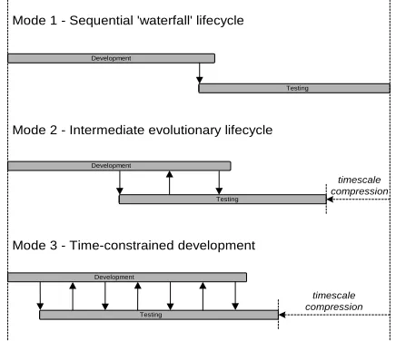
The extent of concurrency and iteration therefore distinguishes time-constrained software

development from more conventional processes. These differences can be illustrated as three

‘modes’ of software development as illustrated in Figure 1.

Mode 1 - Sequential 'waterfall' lifecycle

Mode 2 - Intermediate evolutionary lifecycle

Mode 3 - Time-constrained development

timescale compression

timescale compression

Development

Development

Development

Testing

Testing

Testing

Figure 1: Three Modes of Software Development

Mode 1 represents a sequential ‘waterfall’ model (Royce 1970) of software development that

lays development activities end-to-end. The intrinsic assumption that software can be

developed right-first-time is, however, unrealistic and the resulting timescale is commercially

impractical for many organisations (Boehm 1988).

Mode 2 represents an intermediate evolutionary lifecycle using a limited amount of

problems whilst, in theory, reducing the overall development lead-time. This approach is

typical of conventional software development (Parnas and Clements 1986).

Mode 3 represents the extreme form of evolutionary development that we have observed in

industry. This exploits high levels of concurrency and staged-delivery to meet the time

constraints imposed on the software process, and is based on three assumptions. First, that

concurrency reduces overall development lead-times. Second, that iteration gives rise to

improvements in product maturity. Third, that the benefits of reduced lead-times outweigh

the costs of instability and rework.

The existence and effects of lifecycle concurrency and iteration are, however, largely implicit

in the literature and are treated as an issue of project management rather than an integral part

of the software lifecycle (Blackburn and Hoedemaker 1996). Conventional approaches to

measurement, modelling and management treat the development process as being linear,

sequential and static. Whereas, the industrial practices used to achieve timescale compression

in industry are iterative, concurrent and dynamic.

An important observation is that a schedule delay, or a change in the quantity of work

performed at any point in these lifecycles, has the potential to cause increased allocation of

resource that can affect the performance of later phases. This dynamic behaviour has

significant implications for the way in which software development is modelled

(Abdel-Hamid and Madnick 1991; Lehman 1995). It follows that we need to reassess existing

predictive models for their suitability in time-constrained environments.

3. Conventional Predictive Models

Conventional predictive models take the form shown in Figure 2. For example, COCOMO

takes the user’s predictions of system size and, using 15 productivity drivers (e.g.

programming languages, programmer experience), estimates the level of effort required in

person-months (Boehm 1981). A planning tool, such as Microsoft Project, is then used to

Model Effort (Person-Months) Productivity Drivers

System Size

Figure 2: Conventional Predictive Models of Software Development

In practice, the predictive accuracy of these models is poor even for simple development

projects. As Kitchenham observes “There is no evidence that estimation models can do much

better than get within 100% of the actual effort during requirements specification and 30%

of the actual effort prior to coding” (Kitchenham 1998). The models are even less

appropriate for managing time-constrained software development for a number of reasons.

First, in time-constrained development (i) the timescales of the project, and its major

increments, are largely fixed and non-negotiable, and (ii) the total level of resource remains,

on the whole, quite stable and predictable. Since time and resource (and thus available effort)

are ‘known’ variables, having them as outputs of a predictive model is therefore of little

benefit to planners.

Second, as time-constrained development is a dynamic feedback system, estimating and

planning cannot be treated as separate activities. The ‘point-estimates’ given by conventional

estimation models therefore give little indication of the risks involved in accepting these

constraints because process behaviour is dynamically dependent on the way the process is

planned and controlled, i.e. “a different estimate creates a different project” (Abdel-Hamid

1989).

The intrinsic problems of prediction mean that we need to rethink its rôle in the management

of software development. As Kitchenham observes: “senior managers and project managers

need to concentrate more on managing estimate risk than looking for a magic solution to the

4. A Model of Time-Constrained Software Development

4.1 Overview of Capacity Based Scheduling

We have developed a new model of time-constrained development, called Capacity Based

Scheduling (CBS), which addresses the problems of the lead-time approach. The basic

concept of Capacity-Based Scheduling is to reverse the inputs and outputs of current

predictive models (

Figure 3).

Model Planned Resource (People)

Required Productivity (LoC/Person-Week) Planned Timescale (Weeks)

Planned Product Size (LoC)

Figure 3: Capacity-Based Scheduling – Concept

By making the constraints on resources and timescales explicit inputs, we can reason about

the nature of the capabilities required for their achievement. Critically, we are modelling the

constraints on the process in order to compare the Required Productivity against the Actual

Productivity of past projects, and thus indicate the relative ‘risk’ of alternative plans.

The principles behind the model are best explained by example. Consider two planned

deliveries of code, A1 and A2. Delivery A1 needs 1000 Lines of Code (LoC) to be written and

delivery A2 needs 500 LoC. The work can start on each delivery immediately and the

delivery deadline for each is 10 weeks from now. Supposing we have a staff of six

programmers, how should we allocate staff between the parallel deliveries?

At time 0, delivery A1 requires 100 LoC to be produced each week until the deadline and A2

requires 50 LoC to be produced each week until the deadline. An obvious and well-motivated

approach to allocating staff to the tasks would be to allocate four programmers to A1 and two

programmers to A2. This balances the load between the parallel activities; no programmer is

under-stressed whilst another is overstressed. In other words, this is proportional allocation

Thus, after the first week with the proportional allocation above, the four programmers

working on A1 deliver (together) 100 LoC and the two on A2 deliver 50 LoC. If there are no

other deliveries starting after the first week then the required rates of progress for A1 and A2

are now 900/9=100 LoC per week and 450/9=50 LoC per week, i.e. the same as before. The

same approach can likewise be used for any number of concurrent deliveries; if, for example,

another delivery, A3, started after the first week then we would need to take it into account in

deciding proportional allocations for Week 2.

The Required Productivity at any stage can be compared with historical performance and

judgements made. For example, requiring programmers to have a very high productivity now

could affect the amount of work to be carried out in a later delivery since stressed

programmers might introduce more defects. By modelling planning constraints and

assumptions, the CBS approach highlights what meeting the deadlines actually means for the

staff carrying out the tasks.

4.2 A Formal Description of the Primitive Model

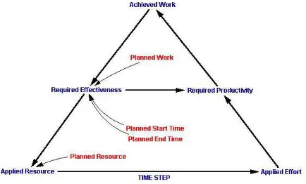
The basic structure of our primitive model is presented in Figure 4 that shows the main

variables and their causal relationships as arrows. The variables are calculated by dynamic

(time-based) equations that describe the relationship between inputs and outputs.

Figure 4: Capacity-Based Scheduling – Primitive Model

The inputs to the model are the Planned Work (LoC) to be produced, the Planned Resource

(people) in each phase team, the Planned Start Time (time), and the Planned End Time (time)

(LoC/week), the Applied Resource (people), the Applied Effort (person-weeks), the Required

Productivity (LoC/person-week), and the Achieved Work (LoC), over time.

The following steps formally describe one cycle of the model’s operation (corresponding to

one unit of time). The full model is implemented using the VenSim simulation environment.

Here we concentrate on the operations of the primitive model introduced to explain the

modelling approach.

Step 1 – Input the Planned Schedule

There are a number of planned deliveries (e.g. D1, D2).

• Deliveries = {D1, …, Dn}

Each delivery comprises several phases of the software lifecycle (e.g. Code, Unit Test).

• Phases = {P1, …, Pn}

The planning window comprises a set of time points of from 0 to T with the current time

being t.

• Time = 0 ... T

• time = t

Each delivery involves planned work required for its completion (e.g. 1000 LoC for D1 and

500 LoC for D2).

• Planned Work : Phase x Delivery → R

(where R is the set of non-negative numbers)

• Each delivery phase has a planned start and end time.

• Planned Start Time : Phase x Delivery → Time

Finally, there is a fixed resource capability available for each phase:

• Planned Resource Phase: Phase → R

(i.e. a natural number of people)

Step 2 – Calculate the Required Effectiveness

After t time steps a certain amount of work has been performed (Work Achieved) for a

specific Phase (p) of each Delivery (d).

• Achieved Work : Phase x Delivery x Time → R

Each product is associated with the remaining required effectiveness at time t.

• Required Effectiveness : Work x Time → R (LoC/time) given by

• Required Effectiveness (p,d,t) = (Planned Work (p,d,t) – Achieved Work (p,d,t)) /

(Planned End Time (p,d)-t)

• if Planned End Time (p,d) > t and 0 otherwise.

The Required Effectiveness shows the total stress on the development team.

Step 3 – Calculate the Applied Resource

At each time interval (t), the Planned Resource for each phase (p) is allocated among parallel

deliveries (d) relative to the Required Effectiveness.

• Applied Resource: Phase x Delivery x Time → R

• Applied Resource (p,d,t) = Planned Resource(p) x (Required Effectiveness(p,d,t)

/

∑

=

=

Dn j

D j 1

Step 4 – Calculate the Applied Effort

• Applied Effort : Phase x Delivery x Time → R

• Applied Effort (p,d,t) = Applied Resource (p,d,t) x t

Step 5 – Calculate the Required Productivity

We are interested in how much the Required Productivity might have to deviate from known

performance in order to meet the deadline.

• Required Productivity : Phase x Delivery x Time → R given by

• Required Productivity(p,d,t) = Required Effectiveness (p,d,t) / Applied Effort (p,d,t)

if Applied Effort (p,d,t) > 0 and 0 otherwise.

Step 6 – Calculate the Achieved Work

The Achieved Work in each time-step is assumed to be the amount required.

• Achieved Work : Phase x Delivery x Time → R given by

• Achieved Work (p,d,t) = Required Productivity (p,d,t) x Applied Resource (p,d,t)

Finally, the Achieved Work to-date for a delivery is given by summing all the achievement

for that product to date.

• Achieved Work To-Date (p,d,t) =

∑

=

=

t j

j 1

Step 7 – Iterate

5. Model Worked Examples

In this section, three examples are shown to demonstrate the operation of the basic model.

The first example, Section 5.1, revisits our example from Section 4.2 to model two

concurrent deliveries for a single lifecycle phase (Code). The second example, Section 5.2,

considers the impact of staging our two concurrent deliveries to start at different points in

time. The final example, Section 5.3, uses the model to study the effect of having staged

concurrent deliveries across two lifecycle phases (Code and Low Level Test). In all cases, the

goal is to evaluate whether the planned schedule is feasible given external constraints and

internal planning assumptions.

5.1 Example 1: Two Deliveries, One Phase

The input to the model is the planned delivery schedule consisting of the: Planned Resource,

Planned Work, Planned Start Time and Planned End Time, for each delivery.

The Planned Resource is the number of available resource (people) for each phase. We

assume that each phase (e.g. Code) contains a fixed pool of staffing resources over the

time-period under consideration. In this example, the Planned Resource is 6 people.

The Planned Work is the total amount of work (LoC) to be performed. We assume that this

plan includes both planned new work and an allowance for planned rework. In this example,

the values of Planned Work are 1,000 LoC and 500 LoC respectively.

The Planned Start Time and Planned End Time are the planned start and end times (week) of

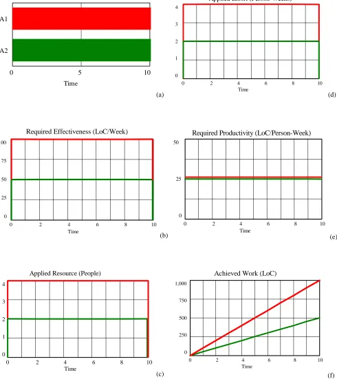
each phase delivery. In this example, both A1 Code and A2 Code start at Week 0 and end at

Week 10 (Figure 5a, situated at the end of this paper).

The model then iteratively calculates the values of Required Effectiveness, Applied Resource,

Applied Effort, Required Productivity and Achieved work.

The Required Effectiveness calculates the average work rate (LoC/week) required to meet the

deadline. We assume that the coders are 100% effective, i.e. our estimates of size are correct

therefore 100 LoC per week and delivery A2 is 50 LoC per week for the duration under study

(Figure 5b).

The Applied Resource is allocated according to the Required Effectiveness over time of the

two parallel deliveries. Our strategy for allocating resources does not take into account other

deliveries with start times in the future but only with the active tasks in the next time step

(week). We assume that deliveries share a common resource team that is allocated by

managers according to the relative size of the task. In this case, the ratio of Required

Effectiveness is 100:50, or 2:1, so the Planned Resource of 6 people is allocated in the ratio

of 4 coders on A1 to 2 coders on A2 (Figure 5c).

The Applied Effort is the product of Applied Resource and Time. We assume a standard

working week with no overtime such that total effort is fixed, therefore the Applied Effort

mirrors the level of Applied Resource. In this example, the Applied Effort is consistent at 4

person-weeks for A1 and 2 person-weeks for A2 (Figure 5d).

The total Required Productivity is equivalent to the Required Effectiveness since we assume

that progress is actually made evenly at the required rate (i.e. all deadlines are met). In this

example, if 25 LoC/person-week is the average Required Productivity calculated for a

programmer after proportional allocation has been carried out, then it is assumed that they

will deliver 25 LoC in the next week (Figure 5e).

The Achieved Work is simply the sum of productivity over time. The simple model therefore

approximates to linear growth in the product (Figure 5f).

The model is simulated over the period of ten weeks (i.e. t=0 to t=10). A manager can then

make assessments to see if the loads on each delivery (A1 100 LoC/week and A2 50

LoC/week), and on the code team as a whole (A1 + A2 = 150 LoC/week), are realistic and

W e e k

1 2 3 4 5 6 7 8 9 1 0 P la n n e d P r o d u c t[D 1 ,C o d e ] 1 0 0 0

P la n n e d P r o d u c t[D 2 ,C o d e ] 5 0 0 P la n n e d S ta rtT im e [D 1 ,C o d e ] 1 P la n n e d S ta rtT im e [D 2 ,C o d e ] 1 P la n n e d E n d T im e [D 1 ,C o d e ] 1 0 P la n n e d E n d T im e [D 2 ,C o d e ] 1 0

Inputs

P la n n e d R e s o u rc e [C o d e ] 6

R e q u ire d E f fe c tiv e n e s s [ D 1 ,C o d e ] 1 0 0 1 0 0 1 0 0 1 0 0 1 0 0 1 0 0 1 0 0 1 0 0 1 0 0 1 0 0 R e q u ire d E f fe c tiv e n e s s [ D 2 ,C o d e ] 5 0 5 0 5 0 5 0 5 0 5 0 5 0 5 0 5 0 5 0 A p p lie d R e s o u rc e [D 1 ,C o d e ] 4 4 4 4 4 4 4 4 4 4 A p p lie d R e s o u rc e [D 2 ,C o d e ] 2 2 2 2 2 2 2 2 2 2 A p p lie d E ffo rt[D 1 ,C o d e ] 4 4 4 4 4 4 4 4 4 4 A p p lie d E ffo rt[D 2 ,C o d e ] 2 2 2 2 2 2 2 2 2 2 R e q u ire d P r o d u c tiv ity [ D 1 ,C o d e ] 2 5 2 5 2 5 2 5 2 5 2 5 2 5 2 5 2 5 2 5 R e q u ire d P r o d u c tiv ity [ D 2 ,C o d e ] 2 5 2 5 2 5 2 5 2 5 2 5 2 5 2 5 2 5 2 5 A c h ie v e d P r o d u c t[D 1 ,C o d e ] 1 0 0 2 0 0 3 0 0 4 0 0 5 0 0 6 0 0 7 0 0 8 0 0 9 0 0 1 0 0 0

Outputs

5.2 Example 2: Two Staged Deliveries, One Phase

The first example considered two deliveries operating in parallel for the entire duration of the

simulation (Example 1). In practice, software deliveries tend to be staged over time in

response to the constraints from upstream phases (e.g. the supply of systems requirements),

the needs of downstream phases (e.g. the availability of code for engine testing), and to

balance the pressure on the development team.

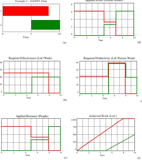
In this example, we consider the impact of staging our two deliveries by delaying the start of

A2 until Week 5, whilst finishing A1 earlier at Week 8 (Figure 6a). We therefore amend the

Planned Start Time and Planned End Time of the deliveries and run our model again to

observe the effects.

The immediate impact of staging the deliveries can be seen in Figure 6b. Having reduced the

available timescale for each delivery, whilst keeping the Available Resource and Planned

Work at the same levels, there is a consequent increase in the Required Effectiveness of both

deliveries.

The effect of the staged deliveries can be seen when we look at the way the Planned

Resource is allocated across the concurrent deliveries as Applied Resource (Figure 6c). All

the available resources are applied to delivery A1 until Week 5 at which time it is split

between A1 and A2 proportionally relative to the required effectiveness of the deliveries.

When delivery A1 finishes, in Week 8, all the available resource is switched to delivery A2.

In simple terms, we are therefore modelling the way a manager might allocate their resources

and the resulting effort profile (Figure 6d).

The key outputs of the model are the Required Effectiveness and Required Productivity

necessary to perform the given schedule successfully (Figure 6b and Figure 6e). If we

compare these results with our earlier example, Figure 5b, we can see that the Required

Effectiveness has increased from 100 to 125 LoC/Week for A1 and from 50 to 100

LoC/Week for A2. The corresponding demands on Required Productivity (Figure 6e) may be

relatively trivial and absorbed by a short-term increase in team performance (due to

problems and overloading. The manager might therefore choose to (i) adjust the profile of

Planned Resource, (ii) adjust the Planned Start Time and Planned End Time of schedule

activities, or (iii) adjust the levels of Planned Work to be performed in each delivery. The

manager can therefore investigate the potential impact of alternative schedules and

constraints.

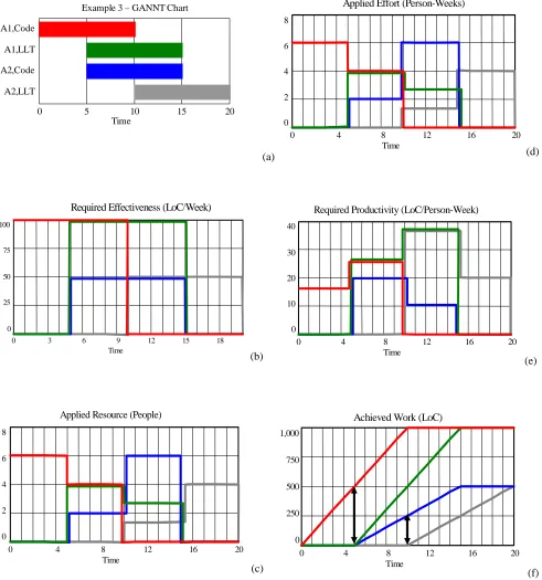
5.3 Example 3: Two Staged Deliveries, Two Phases

Until now, we have only been concerned about one lifecycle phase (i.e. Code). In practice,

we want to model the many levels of concurrency and iteration that we observe in industry.

To do this we need to expand our model to consider all phases in the development lifecycle.

In this example, we consider a planned schedule consisting of two deliveries (A1 and A2)

each with two lifecycle phases, Code and Low Level Test (LLT), over a period of 20 weeks as

shown in Figure 7a. This allows us to model the hierarchy of concurrency.

The operation of the model is the same as we have described in our previous examples. The

Required Effectiveness (Figure 7b) calculates the work rate needed to complete each

individual combination of delivery and phase (e.g. A1 Code, A1 Low Level Test) on time. For

simplicity, we assume in the primitive model that resource cannot move between code and

test phases, reflecting the skills restrictions observed in industry. The level of Applied

Resource thus uses independent resource pools for code and test phases, i.e. Planned

Resource (Code) = 6 and Planned Resource (LLT) = 4. At any point, the available coders are

allocated among parallel coding phases and the available testers are allocated among parallel

testing phases, giving the profile in Figure 7c.

This example illustrates one of the main problems of planning concurrent software

development. The manager must ensure that the work-products of upstream phases (e.g.

Code) are sufficiently mature for downstream phases (e.g. Low Level Test) to begin. If the

upstream work-products are not sufficiently mature then there may be delays in the schedule.

Conversely, if the upstream work-products are “too mature” then we may be missing an

opportunity to further compress the schedule. In this example, the code for both products is

manager then has the option to determine if this level is reasonable or not based on their

observations on past performance.

6. Conclusions

In this paper, we have identified the limitations of current predictive models and proposed a

new approach to modelling time-constrained development, called Capacity-Based

Scheduling (CBS). The problem with conventional models is that they treat estimation and

planning as separate activities. Whereas, in practice, the way a project is planned and

controlled has a significant effect on its performance, i.e. ‘a different estimate creates a

different project’ (Abdel-Hamid 1989).

In response, we have proposed a Capacity-Based Scheduling (CBS) approach to model

concurrency and iteration in a planned schedule. A primitive model was used to explain the

principles behind the CBS approach. By modelling just two phases of two deliveries, we

were able to explain the complexity of interactions in time-constrained projects. A manager

must consider simultaneously the effects of planning decisions on concurrent deliveries in

the same phase, and subsequent phases of the same delivery, whilst trying to minimise the

overall lead-time.

By comparing the levels of required productivity predicted by the model against the actual

productivity, it is possible to evaluate the relative feasibility of a plan. The CBS approach

therefore allows managers to make much more effective decisions as they can investigate the

References

Abdel-Hamid, T. and S. Madnick (1986). "Impact of Schedule Estimation on Software Project Behaviour." IEEE Software 3(4): 70-75.

Blackburn, J. D., G. Hoedemaker, et al. (1996). "Concurrent Software Engineering: Prospects and Pitfalls." IEEE Transactions on Engineering Management 43(2): 179-188.

Boehm, B. W. (1981). Software Engineering Economics. Englewood Cliffs, NJ, Prentice-Hall.

Boehm, B. W. (1988). "A Spiral Model of Software Development and Enhancement."

IEEE Computer 21(5): 61-72.

Kitchenham, B. A. (1998). The Certainty of Uncertainty. European Software Measurement Conference FEMSA 98, Antwerp, Technologisch Institute.

Lehman, M. M. (1995). Process Improvement - The Way Forward. 7th International Conference on Advanced Information Systems Engineering (CAiSE'95), Jvyaskyla, Finland.

Parkinson, J. (1996). 60 Minute Software: Strategies for Accelerating the Information

Systems Delivery Process. New York, John Wiley & Sons.

Parnas, D. L. and P. C. Clements (1986). "A Rational Design Process: How and Why to Fake It." IEEE Transactions on Software Engineering SE12(2): 251-257.

Royce, W. W. (1970). Managing the Development of Large Systems: Concepts and

Techniques. IEEE WESCON, IEEE Press.

Sims, D. (1997). "Vendors Struggle with Costs, Benefits of Shrinking Cycle Times."

Example 1 – GANNT Chart

0 5 10 Time

A1

A2

(a)

Applied Effort (Person-Weeks)

4

3

2

1

0

0 2 4 6 8 10

Time

(d)

Required Effectiveness (LoC/Week)

100

75

50

25

0

0 2 4 6 8 10

Time

(b)

Required Productivity (LoC/Person-Week)

50

25

0

0 2 4 6 8 10

Time

(e)

Applied Resource (People)

4

3

2

1

0

0 2 4 6 8 10

Time

(c)

Achieved Work (LoC)

1,000

750

500

250

0

0 2 4 6 8 10

Time

(f)

0 5 10 Time

A1

A2

Example 2 – GANNT Chart

(a)

Applied Effort (Person-Weeks)

8

6

4

2

0

0 2 4 6 8 10

Time

(d)

Required Effectiveness (LoC/Week)

200

150

100

50

0

0 2 4 6 8 10

Time

(b)

Required Productivity (LoC/Person-Week)

40

30

20

10

0

0 2 4 6 8 10

Time

(e)

Applied Resource (People)

8

6

4

2

0

0 2 4 6 8 10

Time

(c)

Achieved Work (LoC)

1,000

750

500

250

0

0 2 4 6 8 10

Time

(f)

Example 3 – GANNT Chart

0 5 10 15 20

Time A1,Code A1,LLT A2,Code A2,LLT (a)

Applied Effort (Person-Weeks)

8

6

4

2

0

0 4 8 12 16 20

Time

(d)

Required Effectiveness (LoC/Week)

100

75

50

25

0

0 3 6 9 12 15 18

Time

(b)

Required Productivity (LoC/Person-Week)

40

30

20

10

0

0 4 8 12 16 20

Time

(e)

Applied Resource (People)

8

6

4

2

0

0 4 8 12 16 20

Time

(c)

Achieved Work (LoC)

1,000

750

500

250

0

0 4 8 12 16 20

Time

(f)