samples for composition analysis
.
White Rose Research Online URL for this paper:
http://eprints.whiterose.ac.uk/468/
Article:
Tesar, V., Tippetts, J.R., Low, Y.Y. et al. (1 more author) (2004) Development of a
microfluidic unit for sequencing fluid samples for composition analysis. Chemical
Engineering Research and Design, 82 (A6). pp. 708-718. ISSN 0263-8767
https://doi.org/10.1205/026387604774195993
[email protected] https://eprints.whiterose.ac.uk/ Reuse
Unless indicated otherwise, fulltext items are protected by copyright with all rights reserved. The copyright exception in section 29 of the Copyright, Designs and Patents Act 1988 allows the making of a single copy solely for the purpose of non-commercial research or private study within the limits of fair dealing. The publisher or other rights-holder may allow further reproduction and re-use of this version - refer to the White Rose Research Online record for this item. Where records identify the publisher as the copyright holder, users can verify any specific terms of use on the publisher’s website.
Takedown
If you consider content in White Rose Research Online to be in breach of UK law, please notify us by
www.ingentaselect.com=titles=02638762.htm Trans IChemE, Part A, June 2004
Chemical Engineering Research and Design, 82(A6): 708–718
DEVELOPMENT OF A MICROFLUIDIC UNIT
FOR SEQUENCING FLUID SAMPLES FOR
COMPOSITION ANALYSIS
V. TESARˇ*, J. R. TIPPETTS, Y. Y. LOW and R. W. K. ALLEN
Department of Chemical and Process Engineering, The University of Sheffield, Sheffield, UK
A
microfluidic sample-sequencing unit was developed as a part of a high-throughput catalyst screening facility. It may find applications wherever a fluid is to be selected for analysis from any one of several sources, such as microreactors operating in parallel. The novel feature is that the key components are fluidic valves having no moving parts and operating at very low sample flow Reynolds numbers, typically below 100. The inertial effects utilized in conventional no-moving-part fluidics are nearly absent; instead, the flows are pressure-driven. Switching between input channels is by high-Reynolds-number control flows, the jet pumping effect of which simultaneously cleans the downstream cavities to prevent cross-contamination between the samples. In the configuration discussed here, the integrated circuit containing an array of 16 valves is etched into an 84 mm diameter stainless steel foil. This is clamped into a massive assembly containing 16 mini-reactors operated at up to 400C and 4 MPa. This paper describes the design basis and experience with prototypes. Results of CFD analysis, with scrutiny of some discrepancies when compared with flow visualization, is included.Keywords: fluidics; microfluidics; sampling; no-moving-part valves.
INTRODUCTION
Taking samples for composition analysis is an important operation in many chemical engineering processes. Analy-sers tend to be expensive instruments and it is not unusual to use an analyser to process samples from many sources. This also brings the additional advantage of analysing the samples by the same process and the same calibration settings. A flow switching sampling unit (sometimes called a sequencer or multiplexer) is needed, operating according to Figure 1. Of course, samples analysed sequen-tially require slow variations of their composition compared with the sampling frequency, but this is seldom a problem. Of increasing importance are applications of this sequen-tial sampling mode in monitoring reaction products from a number of reactors operating in parallel—Figure 2. The task may be maintaining product quality in a plant achieving the required large production rate by numbering-up rather than scaling-up or the reactors. Another category is the combi-natorial chemistry. This is a field where the tendency is to use small test reactors, perhaps even microreactors (e.g. Ehrfeld, 2000). The small size makes it possible to operate a
large number of tests simultaneously and under identical temperature and other conditions. Of course, also the size of the sampling unit then has to be correspondingly small.
In principle, the sampling unit could be assembled from standard moving part valves (as shown schematically in Figure 2). However, devices such as solenoid valves often rely on components (elastomeric seals, electrical insulation), that degrade and emit contaminants at elevated tempera-tures, which are often typical in these tests—not only to increase the reaction rate, but also to prevent condensation and to enable quenching. Thermal control would be difficult with a complex electromechanical system. Also the size would be incompatible with the dimensions of microreac-tors. As a solution, no-moving-part fluidic valves have been suggested.
Fluidic flow diverter valves are well established (e.g. Priestman and Tippetts, 1984; Tesarˇ, 2004). In the absence of moving parts, the inertia of a jet of fluid, accelerated in a nozzle, can be used to direct it to an appropriate outlet. At a large scale, the fluidic sampling unit may be based upon switching the flow by an array of wall-attachment bistable diverters. Operating in turbulent flow, the Coanda effect causes the jet to cling to either of two attachment walls leading to outlet channels. In the present case, however, the Reynolds number, Re (essentially a ratio of inertial to viscous effects in fluids), is too low for any realistic way
*Correspondence to: Professor V. Tesarˇ, Department of Chemical and Process Engineering, The University of Sheffield, Mappin Street, Sheffield SI 3JD, UK.
of generating a jet-like flow of the sample to use such effects.
This paper describes an alternative approach using pres-sure driven flow in the no-moving-part fluidic valves. The aim was to utilize recent advances of micro-fluidics to build an integrated sampling unit with channels and interaction cavities made by etching in a single component.
THE TASK
In the present case, the sampling unit was developed for use in a high-throughput catalyst testing facility (Adamset al., 2000). The task was to sample small gas flows from 16 small catalytic reactors. The reaction investigated was the Fischer–Tropfsch hydrogenation of carbon monoxide to ethanol, typically at 400
C and at 4 MPa (Wilkin et al., 2002). The sampling unit consisted of 16 valves arranged in a radial array around the central outlet to the analyser. The number 16 was chosen after computer-aided design trials confirmed this to be a suitable number to constitute a generation size for use in genetic algorithm searching techniques. The sampling unit was manufactured as a
single stainless steel foil with the integral fluidic circuit cavities etched into it in a single etching step. The circuit was fed with the necessary supply and control flows by apertures drilled normal in the top and bottom clamping components, and similarly provided on the other side with the vent apertures for dumping the samples not needed at a particular instant of time. Even though for simplicity the states of the valves are here described as ‘Open’ and ‘Closed’, they in fact operated by diverting, damping the sample flow since its interruption in the ‘Closed’ valve would adversely influence the essential requirement of similarity of conditions in all reactors.
The main features of the specification were as follows:
the sampled gas was mixture of hydrogen and carbon monoxide;
the whole flow from any reactor was the ‘sample’, unlike other systems in which just a small fraction was sampled; despite this, the flow rate available—dictated by the reactor residence time—was very small, ca 320109
m3s1
per reactor;
cool nitrogen gas was used as the control medium, fed through an individual line per each valve; hence for the initial designs, no fluidic control logic was needed. the chosen method of manufacture was etching into a
[image:3.595.62.278.66.177.2]stainless steel foil; the best reproducibility was obtained when the etching was done from both sides all the way through the foil, which was then clamped between thick bottom and top cover plates to form the closed channels; the narrowest part of the channel, the nozzles, was in the first prototype of 0.34 mm width; foils 0.25 mm thick resulted in the rather small nozzle aspect ratio 0.735. Later, in the second prototype, the nozzles were made wider, of 0.4 mm width, and the aspect ratio was increased to 1.0 (i.e. the depth being the same as the width, the limit possible with etching) by using 0.4 mm thick foils. This change was required to improve manufacturing reproduci-bility as well as aerodynamic performance.
Figure 1. The developed unit essentially performs a conversion of the spatial separation between fluid samples on the input side into their temporal separation at the output.
[image:3.595.89.505.510.731.2]As a consequence, several severe constraints were imposed on the fluidic valves. The effective Reynolds number in the 0.25 mm deep0.34 mm wide channel, with typical flow velocity 3.8 m s1 and sample gas kine-matic viscosity of 40106m2s1, was only Re¼32. If this flow were emitted as a jet, it would have practically no useful inertia as the flow field would be totally dominated by viscous forces.
An unusual feature of the specified task was the strict requirements of sample purity and elimination of any cross-contamination between them. In particular, it was required to eliminate the presence of other samples in the ‘dead’ cavities between the ‘closed’ state valves and the junctions downstream from them (Figure 3). Even though the sample fluids there were immobile, there was a danger of their possible spread into the tested sample by diffusion or induced motions. This was eliminated by ‘purging’ or ‘cleaning reverse flows’ generated in the valves in their ‘closed’ state.
Another potential area of contamination was the ‘open’ state valve. In contrast to a closed mechanical valve, in which the fluids are separated by solid components, no such absolute separation exists in the no-moving-part fluidic valves. The control fluid was neutral, but even its presence in the sample was unwelcome, placing increased demands on analyser sensitivity. A worse danger was possible uncon-trolled mixing with the fluid in the common vent, into which was dumped all the diverted samples in the ‘closed’ state valves. Although a return of the uncontrolled sample mixture from the vent into the valve was not very likely, it was required to remove even this danger by sacrificing a certain percentage of the sample and forcing it to flow into the vent. A ‘guard flow’ equal to 6% of the supplied total was specified as the amount sufficient to oppose any conceivable contaminating backflow from the vent.
PRESSURE DRIVEN LOWReMICROFLUIDICS
The combination of sub-millimetre size and low flow rates is characteristic for microfluidics (Stone and Kim, 2001; Tesarˇ, 2001). The operating Re range in the ‘open’ state is in the present case some two decimal orders of
magnitude smaller than those typical for conventional no-moving-part fluidics. Devices such as vortex valves and Coanda effect diverters cannot be contemplated since they requireRevalues above 800 for even meagre performance. Vortex valves would not be suitable anyway, since their flow throttling action would interfere with the operation of the reactors.
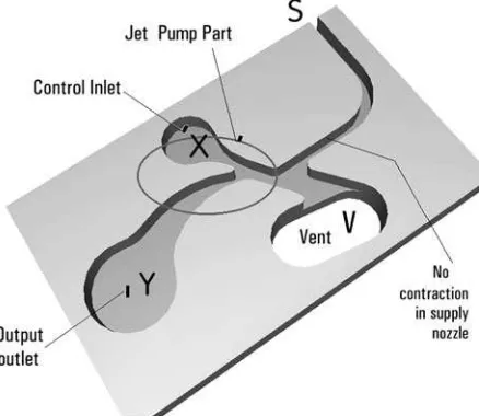
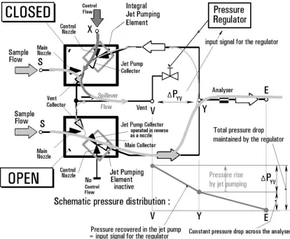
[image:4.595.320.527.67.198.2]In present-day microfluidic devices, the lack of the inertial effects is often circumvented by applying the elec-tro-osmotic flow driving effect. This is, unfortunately, out of question in the present case of the gas as the working fluid. The chosen operating principle was to drive the flow by a constant applied pressure difference, maintained by an external regulator. As presented in the schematic representa-tion (Figure 4) and the practical realizarepresenta-tion of the valve (in its initially proposed form, later changed) shown in Figure 5 (Allen et al., 2000), there are two exits from the valve: a much easier way through the large vent V and the more difficult path through the output terminal Y and the connected analyser. Most fluid would tend to leave through
[image:4.595.58.276.68.210.2]Figure 3.With an array of fluidic valves, it is possible to generate small flows guaranteeing high sample purity. The small reverse flows into the ‘closed’ valve remove all remains of previously tested samples from the inactive channels in the junction circuit. The sacrificed ‘guard’ flow in the ‘open’ valve eliminates possible contamination by fluid from the common vent.
Figure 4.Schematic representation of the microfluidic valve. The flow to the analyser is driven in the ‘open’ state by the applied constant pressure difference DPYV. Its proper magnitude is regulated by turning down the ‘guard’ flow spilled over into the easier way out through the vent V. The jet pumping part is not active.
[image:4.595.316.535.523.713.2]the vent, but this is prevented in the ‘open’ state valves by increased pressure in V relative to the downstream terminal of the analyser. Since the pressure drop across the analyser is constant (the analyser flow rate and its hydrodynamic properties do not vary) and the vent pressure increase is larger than this analyser pressure drop, there is a pressure differenceDPYVbetween Y and V oriented so as to help the
sample to flow towards the Y terminal. Only a small ‘guard flow’ is left to spill over into V. The lower the Reynolds number is, the higher the assisting pressure difference must be. At very low Re, the flow into the analyser is simply pressure-driven rather than just pressure-assisted. This is actually a very effective method which makes possible to force into the output Y irrespective of Re a much higher proportion of supplied flow than is achieved by the jet inertia in the classical fluidics.
The problem is, however, the mechanism of the output flow control required to vary (or to stop completely in the present case of two-positional ‘open’–‘closed’ control) the output flow rate. The control action operates by preventing some (or all) sample fluid from entering the output channel in the valve in spite of the influence of the permanently acting pressure difference DPYV. This is not easy and the
power required for the control action is relatively high. Fortunately, in the present application (and, indeed, in microfluidic flow control in general) the ‘gain’ of the conventional fluidic amplifier context is unimportant. The control flow Reynolds number may be chosen much higher than that of the controlled sample flow, resulting in the ‘fractional gain’, less and even much less than 1.0. The high Recontrol flow is needed to provide the dynamic flow forces capable of carrying the sample fluid away from the output channel entrance.
In the present case, an integral part of the valve is a jet pump (Figure 6) with the output channel connected to its suction port. The control flow thus generates a suction effect which can not only reduce the output flow to zero by overcoming the driving pressure, but can continue beyond, so far that the output flow becomes negative. This results in the required ‘purging reverse flow’.
FIRST PROTOTYPE
[image:5.595.308.540.70.221.2]The initial ideas were influenced by consideration of the hydraulic loss in the ‘open’ flow state. If the sample flow has to leave through the jet pump element (cf. Figure 4), then its complicated path gives rise to loss that is excessive in comparison with the standards of large scale fluidics. An effective jet pump incorporated into the valve, as shown e.g. in Figure 10, presents a really complex ‘open’ flow path. Since effectiveness of small diffusers is generally poor, to say the least, a simplified diffuser-less version according Figure 5 was therefore considered.
At the same time, it is obvious that the reverse flows generated by jet pumping in the ‘closed’ state will be very small. This represents a loss of sample fluid which is taken upstream from the junctions (cf Figure 3). With just a single ‘open’ valve the number of ‘closed’ state valves is large. In the present case of a 16-channel sampling unit, a purge flow in one valve amounting to a mere 3% of the passing sample flow represents in total sacrificing 153¼45%; together
with the additional loss due to the 6% ‘guard’ flow this means a loss of more than 50% of the available reactor flow.
This is near the maximum we can afford in view of the limitations of analyser sensitivity.
As seen in Figure 8 comparing the conditions in the ‘open’ and ‘closed’ state valves mutually connected to form the sampling unit, the magnitude of the pressure loss in the ‘open’ state equals the pressure difference generated by the jet pumping in the ‘closed’ state. This influenced the basic argument in the first prototype design. If the flow through the valve in the ‘open’ state is made easier, producing less pressure drop due to hydraulic losses, then the effectiveness of the jet pumping (required to generate no more than the 3% mentioned above) also need not be high. A design with rudimentary integral jet pump element, as shown in Figure 7 was expected to suffice, since the jet pumping has then to overcome less opposing pressure difference.
A design based upon these ideas, with simplified jet pump—as opposed to the fully fledged jet pump design
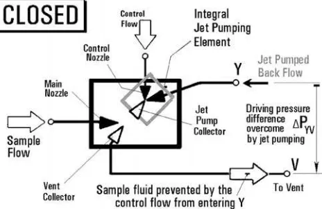
Figure 6.The microfluidic valve shown schematically in the ‘closed’ state. The driving pressure effect pushing the sample fluid into the output Y is overcome by the jet-pumping action of the powerful control jet.
[image:5.595.309.539.495.700.2]shown in Figure 10—was developed up to the stage of a practically tested prototype sampling unit, Figure 11. To give an idea (on a simplified two-channel case) how the driving pressure in the ‘open’ is actually obtained, Figure 9 shows it to be mainly the result of throttling the common vent flow which contains the large control flows of the ‘closed’ valves. This basic idea proved reasonable. There were some problems with reproducibility—the valves were
not identical and the system had to be later complicated by individually adjustable resistors. Some results obtained with these valves were published by Tesarˇ (2001, 2002a, b). The sampling unit could work well, but unfortunately only in the ‘pressure assisted’ regime of Reynolds numbers higher than about 100. This corresponds to a flow rate higher than was actually available from the catalyst testing reactors.
[image:6.595.50.285.65.210.2]Apparently, the quest for low hydraulic losses in the ‘open’ state is valid only in flows with at least some dynamic effects. In the ‘subdynamic’ (Tesarˇ, 2003), pressure-driven regime, entered if the Reynolds number was decreased to the required level aroundRe¼30, the shape of the cavities becomes nearly immaterial. The pressure drop is mainly generated by the friction and a substantial proportion of it on the ‘floor’ and ‘ceiling’ cover plates. This friction com-ponent was high in the low aspect ratio (0.25=0.34¼0.735, cf. Figure 11) channels. The driving pressure required became very high and this was impossible to overcome with reasonable control flow rates in the vestigial jet pum-ping elements. Later evaluations indicated that the control flow rate needed to generate the jet pumping effect would have to be at least 40 times the sample mass flow rate supplied into the valve (in standard fluidics terms this is represents a flow ‘gain’ of only 0.025). With the low visco-sity of the cold nitrogen control gas and the 0.27 mm-wide control nozzle (to get higher control jet velocity, around 55 m s1), the Reynolds number of the control jet was only
Figure 8.Schematic circuit diagram of the simplest version of the sampling unit—with only two valves, one in the ‘open’, the other, in the ‘closed’state. The constant driving pressure differenceDPYVis applied between the two exit terminals.
[image:6.595.88.502.386.728.2]around Re¼1000, just high enough to get some vortex entrainment effect but no real turbulent jet pumping—and yet the attempts to force flow rates of this magnitude resulted in extremely high pressure levels, causing recurrent problems with leaks.
SECOND PROTOTYPE
The disappointment with the first prototype indicated the invalidity of the argument about the advantages of the simplified jet pump shape (Figure 7). Improvement of the reverse flow generating efficiency made possible by incor-porating a full jet pump element with a mixing channel and a diffuser, in line with the idea shown in Figure 9, was clearly a necessity, despite the resulting increase in the required driving pressure difference DPYV to be overcome
in the ‘closed’ state.
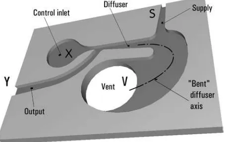
[image:7.595.58.280.67.238.2]Efficiency was also improved by increasing the valve size. The minimum width of the nozzles was enlarged to 0.4 mm. Also the plate thickness was increased to 0.4 mm. The larger channel cross sections and the higher aspect ratio 1.0 eliminated too large a pressure drop rise. Since the new valve plate was to be used with the original neighbouring components, the locations of the terminals were retained. The larger jet pumps, however, did not fit between the existing terminals and this necessitated the somewhat unusual shape with the ‘bent’ axis, as shown in Figure 12. Diffusers of ‘bent’ shape are less effective, but here the ‘bend’ is located very much downstream where the velocities are already low. The larger size of the valves is visible from the photograph of the complete sampling unit, Figure 14, when compared with the original Figure 11. Also the original oval vent holes in the bottom plate were increased by drilling. Their shape became round and this resulted in the changed, rounded shapes of the vent terminals in the sampling unit foil (Figure 11). Fortunately, also the available flow rate from the reactors could be increased somewhat in the second prototype test facility.
Figure 10.Alternative design of the microfluidic valve with enhanced jet pumping effect. Note (in comparison with Figures 5 and 7) the presence of the full jet pump with mixing tube and a long diffuser.
[image:7.595.313.542.71.214.2]Figure 11.Photograph of the first prototype sampling unit containing 16 valves (and also spiral-shaped upstream restrictors). The unit was made by through (two-sided) etching in 0.25 mm thin stainless steel foil. The valves are not extremely small, the main nozzle width being 0.34 mm, but due to the working fluid being high viscosity hot gas at small flow rate, they were operated at very lowRearound 32, typical for microfluidics.
Figure 12. The version of the microfluidic valve used in the second sampling unit prototype. The size was increased and a full jet pump incorporated, with a long diffuser having its axis bent to match the original vent outlet location.
[image:7.595.52.284.521.696.2] [image:7.595.309.539.543.730.2]Despite none of these changes being a substantial one, the result was remarkable. The increased size helped to deal with the manufacturing reproducibility problem. The supply flow Reynolds number rose to Re¼79.2. Also the control
flow required for switching is much smaller. The overall sampling unit performance became satisfactory.
Tests were made not only with the full-scale integrated circuit, but the valve behaviour was also investigated using five-times scaled-up transparent laboratory models, which made possible flow visualization—the Stokes number simi-larity resulting in favourably longer time scales suitable for convenient observation and video recording of the switch-ing, too fast in the full scale. Also helpful were CFD flowfield computations. Fluent 5 with various alternative turbulence models (which, however, did not lead to notice-ably different predictions) was used, mostly with rng hand-ling of low Re turbulence. The computation domain was discretized by an unstructured tetrahedral grid with typically more than 105elements, adapted by refining the grid in the regions of high velocity gradient.
In view of the value Re¼79.2 above, the need of turbulence modeling may sound surprising, but this was necessary for handling properly the powerful control flows which can attain temporarily much higher Re values and indeed reach a turbulent regime (quite welcome, in fact, as the turbulence improves the jet pumping effect).
THE ‘OPEN’ STATE
Typical computed flow paths in the ‘open’ valve as shown in Figure 15 agree very well with laboratory model flow visualizations. The basic problem of this state is adjusting the driving pressure difference DPYV so as to obtain a
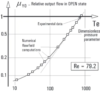
suitable ‘guard’ flow spillover into the vent. This adjustment is helped by finding the dependence between the relative output flow in the ‘open’ no-control-flow state and the
driving pressure difference DPYVas shown in Figure 16.
The quantity plotted on the vertical co-ordinate is the ratio:
mY0¼
_
M MY
_
M
MS (1)
of the output flow into the analyser: MM_Y (kg s1) to the sample flow rateMM_S(kg s1
) from the reactor. The required 6% ‘guard’ flow corresponds to mY0¼0.94. The quantity
plotted on the horizontal axis is the driving pressure differ-ence DPYVnon-dimensionalized to the pressure parameter,
Tegiven by
Te¼DPYV2hb 2
_
M MSn
(2)
whereh(m) is the depth of cavities,b (m) is the nozzle exit width, andn(m2s1) is the fluid kinematic viscosity.
[image:8.595.310.540.65.212.2]Follow-ing the unknown author of the first published discussion of this useful parameter (Anonymous, 2000), this dimension-less quantity may be called the ‘Tesarˇ number’. It is extremely useful in other contexts as well (e.g. Tesarˇ, 2004). For the
[image:8.595.53.283.65.261.2]Figure 14.Photograph of the second prototype sampling unit—again with 16 valves in a radial array—made by etching, this time in a thicker, 0.4 mm stainless steel foil.
Figure 15.Computed pathlines in the second prototype valve in its ‘open’ state. The sample fluid from the reactor (inlet S) passes unhindered into the analyser output Y, with only the small ‘guard’ flow spilled over into the vent V.
[image:8.595.317.530.522.715.2]relative flow magnitudes, of interest in the adjustments, with amY0value near to unity, the dependence found by numerical
computations in reasonable 4% agreement with experi-mental data may be well represented for the discussed valve atRe¼79.2 by the straight line
mY0¼0:00133Teþ0:0622 (3)
It is possible to obtain zero spillover, mY0¼1.0 with
Te¼705 and the desirable mY0¼0.94 with Te¼660, with
the driving pressure difference
DPYV¼ 45:6 Pa (4)
(the negative sign of the result is due to the custom in fluidics of vent pressure being taken as the reference).
[image:9.595.60.272.501.712.2]Another useful view of the problem may be gained form Figure 17. In that case, the computations for the ‘open’ state valve were performed at constant (rather small) values of the pressure parameter Te. It was the supply flow Reynolds number that was varied. The response of the relative output flow mY0 is clearly different at large Re where the small
applied pressure differenceDPYVceases to be important and
all three computed examples tend to follow the common asymptotic line, and at small Re on the sample flow rate wheremY0tends to become constant andRe-independent. In
the former dynamic regime, the valve may be operated without the driving pressure (although the discussed shape Figure 13 is not suitable for this operation mode, in principle a sufficiently high mY0 may be obtained using the kinetic
energy of the jet leaving the supply channel). More inter-esting in the present context is the latter, ‘subdynamic’ flow regime (Tesarˇ 2000, 2003) with self-similar flow patterns, practically uninfluenced by fluid inertia and dependent solely on the pressure driving effect. The existence of a clearly different regime at very low Reynolds numbers has sometimes been questioned—Figure 17, however, demon-strates a well-defined distinct critical transition Reynolds number, Recrit (a suitable definiton of which may be the
minimum mY0value attained with a given constant pressure
parameter value).
Verification experiments were conducted using a scaled-up model in acrylic plastic. The five-times-scaled valve was tested with fluids (air and water) different from those of the actual sampled gas. This provided an opportunity for testing the universality of the dimensionless representation using the variables of equations (1) and (2) of Figure 16. The results were satisfactory. With cold air, the value of the driving pressure for the model was
DPYV¼ 2:11 Pa (5)
evaluated from the conditions of equal Te in equation (3) and equalRe. The experimental spillover magnitude did not differ substantially from that given by equation (3).
THE ‘CLOSED’ STATE AND TRANSFER CHARACTERISTIC
Computations were found to be in very good agreement with experimental data (obtained both with the actual valve and with its scaled-up model) not only in the ‘open’ state but also in the ‘closed’ state. The computed pathlines for the latter are shown in Figure 18. Thanks to the more efficient jet pump part, the cleaning reverse flow in the output terminal was found easily to match the target mY¼ 0.03. As shown in Figure 19, to obtain this state requires relative control flow rate
mx¼
_
M MX
_
M
MS (6)
[image:9.595.310.539.535.705.2][defined in analogy to equation (1)] equal to mx¼9.2, i.e. only a control flow roughly nine-times the sample flow rate as opposed to the estimated (but practically unattainable) relative control flow rate mx¼40 of the first prototype design. Detailed measurements of all 16 component valves revealed differences of 4% of the full range caused by manufacturing tolerances of the etching or misalignments in the assembly process. This magnitude of the deviations did
Figure 17.Reynolds number dependence of the zero control action relative output flow at three different magnitudes of the ‘Tesarˇ number’ pressure parameter. Note the pronounced transition into the subdynamic regime as Redecreases.
not lead to essential problems, but they required a choice of slightly different operational ‘closed’ state with larger nominal return cleaning flows.
With the satisfactory agreements between experiments and numerical flowfield solutions both in the ‘open’ and the ‘closed’ states, it came as a real surprise that the transfer characteristic of computed and experimental steady state points between these two extreme states showed a consider-able disagreement. This is shown in Figure 19, which is a plot of the flow transfer characteristic. The individual states shown there are obtained by admitting gradually increased control flow rates into the control terminal X while the driving pressure difference is re-adjusted at each state to its constant value. The discrepancy has almost no practical consequences, because the real transition between the two end states during the switching is very fast and the unsteady process is certainly different from the succession of steady states. Nevertheless it created a considerable distrust in the computational results—the more difficult to explain since the characteristics evidently consists of two segments and in the first one, called ‘phase A’, the agreement remains equally good as in the fully ‘open’ state. The disagreement is found only in the next ‘phase B’.
The physical difference between the two phases is as follows:
In phase A, as shown schematically in Figure 20 and by flow visualization in Figure 21, the dynamic action of the control flow is so weak that it allows sample fluid (black in the pictures) to flow to the output terminal Y. The relative output flowmYincreases in response to growing input flow as the control fluid is simply added to the flow coming from S. This increase follows the straight line predicted on the basis of absence of dynamic effects in the ‘subdynamic’ regime. Visualization (in the scaled up model, Figure 21) shows the flowfield remaining a smooth, low-Relaminar flow without vortices.
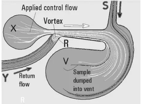
In subsequent phase B, as shown by the computed steady-state pathlines in the crucial central part of the jet pump element, Figure 22, dynamic effects become important.
The momentum of control flow displaces the sample fluid (black) away from the jet pump. Nevertheless, the driving pressure difference DPYVis still strong enough to move
[image:10.595.312.535.73.293.2]some fluid into the output Y. Now, however, it is the control fluid (white) which flows there. In Figure 22 it is seen to be helped in getting to the output channel by the rotational motion of the strong stationary vortex, which is also a dynamic phenomenon. Note that the vortex is held at the left wall L of the output channel entrance. This may resemble the similar dominant vortex computed for the ‘closed’ state, Figure 18. In that case, however, the vortex is attached to the right wall R. Obviously, in the course of the transition process towards the ‘closed’ state the vortex has to move form one wall to the other—which means its
[image:10.595.63.273.533.726.2]Figure 19.Flow transfer characteristic: dependence of the relative output mass flow ratemYon the relative control mass flow ratemX. The switching from ‘open’ to ‘closed’ state progresses through two distinct phases, A and B.
[image:10.595.310.540.548.721.2]Figure 20.Schematic representation of the sample flow (black line) and the control flow (white) in phase A, when the control effect is weak and does not suffice to prevent the sample from reaching the output Y.
location inside the inlet of the output channel cannot be very secure.
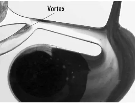
In contrast to the computations, flow visualization has shown the vortex to be present only for a limited duration (fortunately, Stokes number similarity slows the speed in scaled-up models, especially with lower viscosity fluids so that there is enough time for the vortex to be observed, Figure 23). Later, the vortex is shed, carried away with the flow (Figure 24). In its absence, the control fluid is no more helped into the output channel. This explains the observed lower than computed output flow rate. What seemed to be a spectacular failure of the numerical predictions was found to
be due to the steady-state simulation misrepresenting the time-dependent vortex shedding.
CONCLUSIONS
A sampling unit has been developed, producing at its output a sequence of samples for delivery to a destination such as a composition analyser, with an array of microfluidic valves as its key components. Because of very lowRe, due to handling hot gas in small available flow rates, these no-moving-part valves rely on pressure driving the sample in one, ‘open’ valve. In the remaining valves of the array this is neutralized by the powerful, high Recontrol flow of inert gas and by its entrainment effect generated in an integral valve part shaped as a jet pump. The task was complicated by the requirements to generate additional purging and protective flows to eliminate cross-contamination between the samples.
In this context ‘high performance’ has an unusual aspect. In fluidic amplifier terms the valves have flow and pressure ‘gains’ that are very poor, much less than unity. Yet the unit meets demands—the small size, low cost achieved by being made in a single by manufacturing step, resistance to high temperature, small handled flow rates, and the requirement of extreme sample purity—which would be too severe for conventional devices.
REFERENCES
Adams, C., Tesarˇ, V., Allen, R.W.K., Tippetts, J.R. and Low, Y.Y., 2000, High throughput catalyst testing: a novel multichannel microreactor with microfluidic flow control system, in8th NICE (Network for Industrial Catalysis in Europe) Workshop on Fast Analytical Screening of Catalyst and Fast Catalyst Testing, Espoo, Finland, September 2000.
Allen, R.W.K., Tesarˇ, V. and Tippetts, J.R., 2000, Fluidic valve, British Patent Application GB 0003969, March 2000.
Anonymous, 2000, High throughput catalyst testing project,iAc Newsletter, October: 8. Available at: www.iac.org.uk/download/newsletter5.pdf. Ehrfeld, W., 2000, Microreaction Technology: Industrial Prospects
(Springer, Berlin, Germany).
[image:11.595.308.541.63.237.2]Priestman, G.H. and Tippetts, J.R., 1984, Development and potential of power fluidics for process flow control,Chem Eng Res Des, 62(2): 67. Figure 22.Computed flowfield in the phase B is dominated by the large
[image:11.595.54.283.66.290.2]standing vortex attached to the left wall of the output channel entrance. It the control fluid in its getting into the output channel.
Figure 23.Photograph of visualized flow in the model valve immediately after an increase of the control flow to set up the phase B conditions. The standing vortex in the output channel entrance is visible as it retains the dark sample fluid previously present (in the ‘open’ state, cf. Figure 15) in the output channel.
[image:11.595.52.284.528.704.2]Stone, H.A. and Kim, S., 2001, Microfluidics: basic issues, applications, and challenges,AIChE J, 47(6): 1250.
Tesarˇ, V., 2000, Asymptotic correlation for pressure-assisted jet-type micro-fluidic devices, inProceedings Topical Problems of Fluid Mechanics 2000(Institute of Thermomechanics AS CR, Prague, Czech Republic), 85.
Tesarˇ, V., 2001, Microfluidic valves flow control at low Reynolds numbers, J Visual, 4(1): 51–60.
Tesarˇ V., 2002a, Microfluidic turn-down valve,J Visual, 5(3): 301–307. Tesarˇ, V., 2002b, Sampling by fluidics and microfluidics,Acta Polytech J Adv
Eng, 42(2): 41–49.
Tesarˇ, V., 2003, Subdynamic behaviour of pressure-driven microfluidic values, Paper no. 192, inProceedings of 7th Triennial International Symposium on Fluid Control, Measurement and Visualization FLUCOME ’03, Sorrento, August.
Tesarˇ, V., 2004, Fluidic valve for reactor regeneration flow switching,Trans IChemE, Part A, Chem Eng Res Des, 82(A3): 398–408.
Wilkin, O.M., Allen, R.W.K., Maitlis, P.M., Tippetts, J.R., Turner, M.L., Tesarˇ, V., Haynes, A., Pitt, M.J., Low, Y.Y. and Sowerby, B., 2002, High throughput testing of catalysts for the hydrogenation of carbon monoxide to ethanol, in Principles and Methods for Accelerated Catalyst Design and Testing, Derouanne, E.G. et al. (eds) (Kluwer Academic, Dordrecht, The Netherlands), pp 293–303.
ACKNOWLEDGEMENT
Development of the microfluidic sampling unit was supported by Project ‘High Throughput Catalyst Testing’ financed by iAc, the Institute of Applied Catalysis, London, UK.