Parallel processing strategies for solving differential equations and approximation problems

Parallel Processing Strategies

For Solving Differential Equations

And Approximation Problems

Lujuan Chen

November 1995

A thesis submitted for the degree of

Doctor of Philosophy

Statement of Originality

These doctoral research were carried out with Professor E.V.Krishnamurthy as supervisor, and Professor Richard Brent and Dr. Markus Hegland as advisors.

The work presented in this thesis is the result of original research carried out by myself, in collaboration with others, while enrolled in the Computer Sciences Laboratory as a Doctor of Philosophy student.

It

has not been submitted for any other degree or award in any other university or educational institute.

Lujuan Chen

D

Acknowledgements

I wi h particularly to thank my supervisor, Prof. E. V. Krishnamurthy, for his direct guidance throughout the whole of this PhD program. His encouragement,

pa-Li nc and xpert guidance have made this thesis possible. Without his kind support and unwavering confidence in me, I would have never started this project. In par-ticular, I have benefited from his wide-ranging experience, great enthusiasm and his

parkling ideas. Special thanks for his kindness, understanding, and support which have always warmed my heart, especially in my difficult time.

I feel deeply indebted to my advisor Prof. Richard Brent for his professional guid-ance which have benefited me greatly through my all PhD study. Whenever I brought questions to him he could always satisfy me with sorts of ideas and suggestions. He ha always encouraged and supported me to pursue my research career whenever I have encountered research and personal difficulties. Otherwise I could never have finished this project.

I greatly appreciate Dr. Markus Hegland many hours spent proof reading this h s1 and his comments and suggestions on the thesis have been very valuable.

Many thanks go to the co-authors of my publications. I have benefited from their cooperation and valuable suggestions.

I would like to give special thanks to Prof. Li-shan Kang, for his valuable sug-g tions and discussions durinsug-g the period he was workinsug-g in Australian National

ni v rsi ty.

It

is my plea ure to thank my fiance Yanjie Wang, for his love, care, great under-t anding warm encouragemenunder-t, and all under-the emounder-tional supporunder-t he provided.

Finally, I acknowledge with gratitude the support of an Australian National Uni-v r ity cholar hip.

Abstract

The n ed for effective parallel methods for solving problems in science and

engi-n ring i well recognized. Not only do we require algorithms which map well onto practical parallel machines, we also need methods which have well understood con-v rgence and stability properties . In this thesis we decon-vise techniques and parallel algorithms for solving differential equations and for data approximation, the two fun-damental building blocks in scientific and engineering computing .

In Part I , Parallel Processing Strategies For Pratial Differential Equa-t ion s are studied . These researches result in the fo llowing techniques and algorithms:

>-

An improved parallel symmetric domain decomposition method is developed.

..

11

Because of the limited inter-processor communication, this new method is well suited to distributed memory parallel architectu res; also it can scale up effi-ciently to a few tens of processors. Numerical simulation results confirm the con-clusions about the effectiveness of the symmetric domain decomposition method and its parallelization .

>-

An overlaid tree network is introduced to solve partial differential equations.

It

offers further possibilities for concurrency at a fine-grained level. A substantial increase in the speed of many classes of PDE's has been achieved when the concepts of operator splitting and parallel solution of tridiagonal systems via

uffix computations are implemented appropriately.

In Part II , parallel algorithms for (1) generalized inversion, (2) the least squares probl m, and (3) rational interpolation and Pade Approximation are studied. Ap-proximation by means of sp lines is also considered. As a result of these studies we develop th following algorithms and techniques:

>-

deterministic iterative algorithm called Successive Matrix Powering and

Ill

its accelerated schemes for computing both the generalized inverse A+ and rank of matrix a A E cmxn . For very well conditioned matrices, this algorithm

enables calculation of both the generalized inverse and the rank of A in time O(log(m

+

n))

with relative error bounded by any E E (0, 1), independent of matrix size.

>-

A suffix parallel algorithm for calculating Rational Interpolation and Pade Approximation. In this parallel algorithm we construct the continued fraction or Pade approximation as an overlaid tree network with n

+

1 inputs, using Thiele's reciprocal differences. With an M / M Pade approximant (

M

= (

n

+

1)/2, n odd,

!VI=

n/2, n even), this algorithm allows the Pade coefficients to be computed in

0(

n

log

n)

t ime using

0(

n/

log

n)

processors. Interpolated values can then be obtained in O(log

n)

time using the same number of processors .

>-

The techniques of interpolation using smoothing spline surfaces. The questions of description, solution and uniqueness of smoothing spline surfaces are con-sidered. We use Bilinear, Bicubic, and Quasi-bicubic patches in an integrated framework to approximate the three models proposed in this chapter and lead to ome efficient and convenient methods of surface fitting. Parallel algorithms for constructing the smoothing splines are also developed.

.

IV

Preface

his thesis is organized into 8 chapters.

~ Chapter 1 introduces the topics and problems considered in this thesis. Essen-tially, it presents an overview of the thesis.

~ Chapter 2 presents an improved symmetric domain decomposition method in a general theoretical form, and provides a parallelization scheme to achieve a better balance of computation across the individual processors.

~ Chapter 3 considers the decomposition of multidimensional partial differential equations into sets of one-dimensional equations. Then an overlaid tree network i used to solve these locally one-dimensional equations.

~ Chapter 4 provides a domain decomposition approach to Row Projection (RP) methods.

~ Chapter 5 develops a successive matrix powering method to compute both the g n ralized inverse A+ and rank of a matrix A E cmxn. Several improved

schemes are considered to accelerate the method.

~ hapter 6 provides a parallel algorithm to compute Rational Interpolation and Pade Approximations.

~ hapter 7 presents the general theory of interpolation using smoothing spline urface . The questions of description, solution and uniqueness of smoothing pline urfaces are considered .

The quations, sections and figures in this thesis are numbered chapterwise. For ready reference, a glossary of ymbols and commonly used abbreviations are provided before the Contents. The references are arranged in the order of th ir appearance and are listed in the Bibliography.

Mo t of the research work reported in this thesis have already been published or submitted for publication in technical journals. A list is given below:

<i> hen, L., Macleod, I. D. G. and Krishnamurthy, E. V., Suffix parallel com-putation and operator splitting for fast solution of PDE's, Neu,al) Pa,allel ef

Scientific Computation, Vol. 1(3), Sept. 1993, pp. 287-300.

<i> Chen,

L.,

Krishnamurthy, E. V., and Macleod, I. D. G., Generalized Matrix In-version and Rank Computation by Successive Matrix Powering, Pa,allel

Com-puting, Vol.20, (1994), pp. 297-311.

<i> Chen,

L.,

Macleod, I. D. G., On the Parallelism of the Symmetric Domain Decomposition Method, P,oc. of Supe,computing Symposium )92 Canada, June 7-i0,1992, pp. 357-365

<i> Chen,

L.,

Krishnamurthy, E. V., and Macleod, I. D. G., Suffix Parallel Compu-tation for Rational Interpolation and Pade Approximation, P,oc. of

Supe,com-puting Symposium )92, Canada, June 7-10,1992, pp. 318-327

<i> Chen,

L.,

Macleod, I. D. G. and Krishnamurthy, E. V., Parallel solution of partial differential equations using a locally one-dimensional method, P,oc. 1 ~h

Au t,alian Compute, Science Confe,ence, Griffith University, February 1993 ,

pp. 11-1

<i> hen,

L.,

Krishnamurthy, E. V. and Macleod, I. D. G., Generalized Matrix Inver ion and Rank Computation by SMS P,oc. of the 1993 Inte,national

Confe,ence On Pa,allel P,oce ing Vol. 3, Algo,ithm and Applications, .S.A., August 1993.

.

Vl

~ hen L. and Krishnamurthy, E. V., Stability and Convergence of Newton-Lik Methods for Generalized Inversion and Rank Computation, submitted for publication.

~ Chen, L. , Kang, L., Macleod , I. D. G., and Chen Y., Asynchronous Parallel Algorithms Based on DDM on CM-5 for Solving Nonlinear Elliptic PDE's (II), accepted for publication.

~ Chen, L., and Macleod, I. D. G., Algorithmic Principle of Smoothing Spline Surfaces: Part I- Bilinear Case, submitted for publication.

~ Chen, L., Algorithmic Principle of Smoothing Spline Surfaces: Part II - Cubic Case,· submitted for publication.

~ Chen, L., Algorithmic Principle of Smoothing Spline Surfaces: Part III - Quasi-cubic Case, submitted for publication.

A*

II A

11 2

DDM-1

DDM-2

DDM-3

D

3

_M-l

D

3

M-2

DDM

LSP

ODM

PDE

RI

RPM

SDD

SDM

SMP

SMS

sss

SyDM

u(P)

llx

112

Glossary

The complex conjugate transpose of matrix

A.

Euclidean matrix norm

=

max

II

A x 112 /

II

x 112

x fO

The set of m by n complex matrices. Domain Decomposition with overlapping Domain Decomposition without overlapping Domain Decomposition with pseudo-components

Discretised Domain Decomposition Method with overlapping Discretised Domain Decomposition Method without overlapping Domain Decpmposition Method

Least Squares Problem

Operator Decomposition Method Partial Differential Equations Rational Interpolation

Row Projection Methods

Symmetric Domain Decomposition Space Decomposition Method

Successive Matrix Powering Successive Matrix Squaring Smooth-Spline Surfaces

System Decomposition Method

The spectrum of matrix P, or the maximum eigenvalue of matrix P

pT

Euclidean vector norm

= (

x T x ) 1/2

..

1,

1: II

Contents

Acknowledgements

Abstract

Preface .

Glossary

1 Introduction

1.1

1.2

General B ackground

Domain Decomposition Strategies

1.3 Generalized Inverse and Rank Computation

1.4 Suffix Parallel Computation

1.5 Smoothing Splines

1.6 Thesis O utline . . .

I

Parallel Processing Strategies For PDEs

1

..

11

lV

..

Vll

1

1

3

6

7

8

10

12

2 Sy mmetric Domain Decomposition M ethod Wit hou t Ov e rlap 13

2.1 Introduction . . . .

2.2 Th Improved SDD Method

2.2.l ontinuous Equation

13

14

CONTENTS

2.2.2 Discrete Equation . 2.3 Strategy of Parallelism . .

2.4

2.3.1 2.3.2

Case of Two Processors . Case of Four Processors Numerical Simulation . . . .

3 Space Domain Decomposition Scheme for PDE's

3.1 3.2 3.3 3.4

Introduction . . . . Locally One-Dimensional Method

Transformation of Tridiagonal Systems for Suffix Computation U nshuffle Algorithms

3.5 Numerical Examples 3. 6 Full Recursive Doubling

3.7

3.

3.6.1 3.6.2

Specification . . Implementation

3.6.3 Implementation on Multicomputers 3.6.4 Multicomputer Performance Analysis

Implementation on General-Purpose Architectures .

D. lSCUSSIOn . . . . .

.

lX 16 17 17 19 21 25

25

26 30 31 35 37 37 38 41 44 46

48

4 Domain Decomposition for Large Nonsymmetric Linear systems 51

4.1

4.2

4.3

4.4

Introduction . . . . Row Projection Methods (RPM) Row Partitioning Goals . . . . Domain Decomposition for Parallelism

51

52

54

ONTENTS

4.5 The BLock-SSOR method 4.6 umerical Experiments . 4. 7 Discussion . . . .

61 64

69

II Parallel Processing for Approximation Problems

71

5 Generalized Matrix Inversion and Least Squares

5.1 Introduction . 5.2 Notation . . .

5.3 The Successive Matrix Squaring Algorithm . 5.4 Acceleration of Convergence . .

5.4 .1 Acceleration by Scaling .

5.4 .2 Use of Cubic and Quartic Polynomials 5.5 Stability of the SMS and Modified Schemes. 5.6 Complexity Analysis . . . .

5.6 .1 The Complexity of SMS

5.6.2 The Complexity of Modified SMS Methods . 5. 7 Numerical Examples of SMS method

5.7.1 Square Non-Singular Matrix .

5.7 .2 Rectangular Complex Matrix with Reduced Rank 5.7.3 Ill-Conditioned Matrices . . . .

5.7.4 Matrix with Equal Eigenvalues

5. T st Results for the Improved SMS Algorithm 5. CM-5 Implementation Results . . . .

ON TEN TS

,5.10 A Variable Precision Approach

5.10.1 Implementation on DAP-510 Machine. , .10.2 Experimental Results .

5.11 Discussion . . . .

6 Suffix Parallel Computation:

Rational Interpolation and Pade Approx imation

6.1 Introduction . . . . . 6.2 Rational Interpolants

6.3 Computation of the Coefficients 6.4 The Substitution Operation 6.5 Algorithm 1

6.6 Algorithm 2

6. 7 Generalization to Bivariate P ade Approximants

6. Discussion . . . .

7 Smoothing-Spline Approximation of Surfaces

7.1 Introduction . . . .

7. 2 Approximation by Bilinear Smoothing-Spline Surfaces . 7.2.l Construction of Bilinear Smoothing-Spline

7.2.2 Computing the Bilinear Smoothing-Spline 7 .3 Approximation by Bicubic Smoothing-Spline Surfaces

7.3.1 7.3.2

on truction of the Bicubic Smoothing-Spline Surface . omputing the Bicubic Smoothing-Spline

7.4 Qua i-cubic Smoothing- pline . . . .

ONTENTS

7.5 Mapping onto Parallel Machines 7 .5.1 Rational Recursion

7.5.2 Implementation 7.6 Numerical Examples 7. 7 Discussion . . . .

Conclusion

.1 Overview of the Thesis

.2 Details of Contributions

.2.1 New Theoretical Results and Algorithms .2.2 Applications . . . .

. 3 Areas of Current and Further Research

.3.1 Overlapping Decomposition Method for Burgers Equation . . . .

.3.2 Extrapolation of the SMS method .

.3.3 Other Areas for Further Research and Applications

Bibliography

..

Xll

146 147 148 152

156

158

158 160

160

163

165

165

166

168

List of Figures

1.1 The structure of overlaid tree network . . . 8

3.1 3.2 3.3 3.4 3.5 4.1 4.2 4.3 5.1

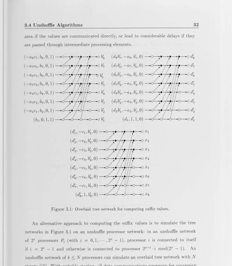
Overlaid tree network for computing suffix values.

Unshuffie processor network for N

=

8 and k

=

4. Sequence of computations on unshuffie network . .

The full-recursive-doubling procedure for produce of eight numbers ..

Data distribution for program Rational-Recursion

NatOrd-BRP NatOrd-BRP BRP-2 . . . .

Distribution of iterations over different precisions

32 33 33 39 43 57 58

60

108 5.2 Speed up as a function of matrix size in variab le precision model 109

6.1

6.2

.3

.4

6.

etwork for computing ai

twork for computing interpolated values etwork for computing aii .

twork for computing aku .

etwork for computing bktk .

.

LIST OF FIGURES

XIV

6.6 Network for computing a i l

6.7 Example calculations with l

=

1 and l

=

2 6. etwork for computing bkt . .

6.9 N twork for evaluating

roi( x)

6.10 ystolic tree network for computing full-order interpolant

7.1 Surface of u1, before smoothing, c E [-0.03, 0.03]

7.2 Bicubic smoothing spline approximating u1 with a

=

0.03 and p

=

0.0279 . . . .

7.3 Surface of u2 before smoothing, c E [-0.05, 0.05]

7.4 Quasi-Cubic smoothing-spline approximating u2 with a

=

0.03 and

p

=

0.0126.

120

120

121

121

123

153

153

154

154

7.5 Surface of u3 before smoothing, c E [-0.0~, 0.03] 155 7.6 Bicubic smoothing-spline approximating u3 with p

=

0.01239. 155

II

List of Tables

2.1 Two processors for problem (2.12) . . . 22 2.2 Four processors for problem (2.17 ) - central difference approximation to

Neumann boundary conditions . . . 23

2.3 Four processors for problem (2.17) - forward difference approximation to

Neumann boundary conditions . . . 23

4.1 Comparison of row partitionings . . . .. . . 61 4.2 The condition numbers for the matrices obtained from the model

prob-4.3

4.4

4.5

4.6

lems . . . . umerical results for model problem 1 umerical results for model problem 2 Numerical results for model problem 3

Comparison of the three partitionings n

=

96 .

67

67

67

67

68

.1 Re ult of the test. . . 101

5.2 Time to multiply a 32 x 32 matrix with a 32 element vector and t o multiply

II

Chapter 1

Introduction

1. 1

General Background

I

The

I

advent of practical digital computers some forty years ago had a profound impact on the study of problems in science and engineering. Problems which had previously been too complex, tedious or error-prone to solve manually became easily amenable to numerical solution. This advance uncovered shortcomings in the exist-ing mathematical theory underlyexist-ing discrete approximations to continuous problems:

veral previously discovered popular difference schemes failed to converge when they

w re applied to larger meshes and more complex physical phenomena. These short-omings motivated a period of intensive research on the stability and convergence properties of difference schemes, leading to various equivalence theorems and

con-. pts such as weak stability and strong smoothnesscon-. As a result of this research, Lh strengths and limitations of various discretization and difference schemes are now b tt r understood.

1.1 Ge n e ra l B ackgrou nd

structural analysis, and nonlinear optics. Nevertheless, the frontiers of research in certain areas are still at least partially defined by the speed and cost of numerically inL nsive computations.

Increasing the computational speed using much faster processors is becoming im-p ssibl due to fundamental im-physical limitations, such as those imim-posed by the sim-peed

flight and the rate of heat generation/removal, not to mention economic and practi-al limitations of opticpracti-al lithography. The best current prospects for increased overpracti-all p ed of solution at reasonable cost lie in the use of parallel computation, where mul-tiple r latively inexpensive processors work in concert to reach an overall solution.

The initially expected gains through parallel computation have proved difficult to r alize for general purpose computation, because of problems involved in synchroniza-tion, data communicasynchroniza-tion, memory contensynchroniza-tion, programming, languages, compilers and load imbalance between processors . Fortunately, many scientific and engineering problems have some common characteristics which make them potentially quite suit-able for parallel solution : computations are usually carried out on a discrete regular grid; the computations are both position and data independent, being essentially the ame at each grid point; and only a small neighborhood of local data values is used in the calculations at each grid point. Thus, we find that problems in this class were among the first to be tackled effectively using parallel computation.

Difficulties with parallel solution of large-scale scientific and engineering problems till ari e however:

• first the simple approach of apportioning ub-spaces of grid points to sepa-rate processors involves exchange of boundary point data values at the end of each iteration or time step, with the attendant delays and need to synchronize proc ors prior to this exchange·

• econd memory address paces are u ually laid out in a more or less linear ( one-dim n ional) fashion whereas many cientific problems are usually posed in two three or four dimen ions. This means that in shared memory parallel

1.2 Do main D ecom p osition Strategies

architectures, neighboring grid point values may be widely separated 1n the memory space;

• third, in relation to the increasing scale and complexity of problems being solved rather than their parallel solution as such, further development of the underlying mathematical theory is required to improve convergence and stability. This is esp cially true of problems such as weather forecasting where extrapolation of known current values (perhaps of limited accuracy) as far as possible into the future is desired.

Th re are two main issues which remain to be addressed in proposing parallel solution m thods for problems in mathematical physics. Ideally, we would like to use the "di-vi de and conquer" strategy, i.e. di"di-vide the overall problem into independent subprob-1 ms which are then solved by loosely-coupled processors, to minimize inter-processor synchronization and communication, and obtain the final solution as a combination of the· subproblem solutions. In dividing the overall problem into subproblems and th n solving these independent ly, we need an efficient mapping of algorithms onto

c mputational structures to ident ify the potential concurrency.

This thesis focuses on these two issues of division into relatively independent ubproblems and development of efficient algorithms which take advantage of further l v ls of concurrency within processing nodes for solving the subproblems. In line with current trends in numerical mathematics, the emphasis is on solving classes of pro bl ms ( rather than particular problems) and on standardization.

1 .2

Domain Decomposition Strategies

Th fundamental principl of decomposition methods is to reduce complicated math-matical phy ics problem to a eries of simpler and theoretically better developed problem allowing effective algorithmic realization on modern parallel computer .

The theory of Domain Decomposition as a foundation of parallel algorithms for

1.2 Domain Decomposition Strategies

solving mathematical problems on MIMD and SIMD machines has been followed with gr at interest. Since 1987, a yearly international conference has been held in France xclu ively on the Domain Decomposition Method, motivating more and more re-s archerre-s to become interere-sted in thire-s field. By now the DDM ire-s not only a particular

omputational method, but more importantly also provides a framework for concep-Lualizing and solving classes of problems. The DDM provides a basic "divide and

onquer' strategy for development of parallel algorithms. Some of the issues which motivate research within the DDM framework are: techniques for decomposing do-mains; specification of pseudo-boundary conditions; use of different mathematical rn thods and approximation methods in different sub-domains; use of efficient solvers within sub-domains; computer memory limitations and suitability for implementa-tion on parallel computers; and the balance of computaimplementa-tions between the individual processors.

There are three main Domain Decomposition Methods [45) [12), which can be combi ned if necessary:

(1) Domain Decomposition with overlapping ( DDM-1);

(2) Domain Decomposition without overlapping (DDM-2); and (3) Domain Decomposition with pseudo-components (DDM-3).

Within each of the above major categories we can distinguish several different forms : Discretized Domain Decomposition Method with overlapping (

D

3M-1) or Grid omain Decomposition Method, Space Decomposition Method (S DM) , Operator De-omposition Method (ODM), and System DecDe-omposition Method (Sy DM ) .

DDM-1 and

D

3_{M-1 are fundamental techniques for construction of asynchronous} parall 1 algorithms for MIMD machines, with the following advantages [43) [35) [34)

(q4):

• the multiple procedures formed according to the algorithms are only weakly int rd pendent - only information relating to the pseudo- boundaries needs to be xchanged, reducing communication overheads;

1.2 D omain Decomposition Strategies

• because of the flexibility of the decomposition method, the number of decom-pos d ubproblems can be varied to suit the execution architecture and the load can be balanced by distributing the subproblems appropriately;

• chaotic relaxation can be used on

MIMD

architectures, avoiding synchronization overheads; and

• these techniques are fault tolerant in that occasional errors in data commu-nication between processors can be corrected automatically by the algorithms without affecting the final result.

The DDM-2 and Discretized Domain Decomposition Method without overlapping ( D3M-2), (methods are mainly used to construct synchronous algorithms on MIMD and SIMD architectures. Theoretically we use the substructuring elimination method Lo eliminate unknowns in sub-domains first, then solve the low order linear systems onsisting of unknown points on pseudo-boundaries. Finally, back-substitution gives Lh grid point values inside each subdomain.

If

we use direct metho.ds to solve systems onsisting of unknown points on pseudo-boundaries, the method converges automat-ically. Therefore, DDM-2 and D3M-2 can be used to handle a wide range of linear partial differential equations. In practice, we often use iterative methods to get the olution on pseudo-boundaries instead of explicit elimination, for example, via the pr -conditioned conjugate gradient method. The disadvantages of D3M-2 are that

w cannot use it to get efficient solutions to mathematical physics problems with

complicated domains and that the parallel programs which implement this method ar both difficult to program and have high synchronization overheads.

Symmetric Domain Decomposition (SDD) [64] [67] in theory results 1n a large potential sp edup through parallelism. An improved scheme of SDD [70] [50] greatly r duces he computation time required by the original algorithm. The parallel

effi-i ncy i however reduced due to the load imbalance arising from the different types

f boundary conditions used in the ubproblems.

1.3 Ge n e ra lized Inverse and R ank Computation

and also provide a parallelization cheme to achieve a better balance of computation a ross the individual proces ors.

In hapter 3 decomposition of multidimensional partial differential equations into of one-dim nsional equations is considered. An unshuffie network is introduced to mpute in parallel the suffix recurrence relation to solve the locally one-dimensional problems.

Chapter 4 provides a domain decomposition approach to row projection partition-ing so that parallel implementations of the algorithms are suitable for a wide range of

omputer architectures. The level of concurrency and size of the created subtasks can b chosen to suit the target machine, and the resulting algorithms have advantages over standard domain decomposition methods.

How to solve least square systems or compute g-inverses efficiently is considered n xt since subsystems are least square equations after row part ition ing. Usually the l ast squares systems are ill-conditioned and hence present considerable difficulties. This was the initial motivation for studying more efficient and stable parallel algo-rithms of g-inverse computations. As a result, Newton-Like Methods are developed in Chapter 5.

1.3

Generalized Inverse and Rank Computation

Th g-inverse and rank of A have many applications in statistics, prediction theory, ontrol system analysis, curve fitting, etc .

In 1955 Penrose [59] showed that for an arbitrary finite matrix A E

cmxn,

there a unique matrix X satisfying the set of equations:

AXA= A, XAX = X (AX)*= AX (XA)* = XA ( 1.1)

'\ T .

• '\. 1 ommonly known a the generalized inverse (g-inverse in abbreviated form) and i often d not d by A+, which reduces to the conventional matrix inverse A-1 _when

1.4 Suffix Parallel Computation

is square and non-singular.

ince 1962 sequential algorithms for computing the generalized inverse have been known [62] [5] [ ] [49], but implementation of a parallel algorithm has only recently b n reported [48].

In Chapter 5 we present a deterministic iterative algorithm and several improved . rhemes for computing both the g-inverse A+ and rank of matrix A E cmxn. This

algorithm (SMP) is obtained by generalizing a repeated squaring algorithm to higher powers. The iterative steps in the computation are performed in sequence; each step omprises log₂ l parallel matrix multiplications, where l is the power to which the matrix is raised. For very well conditioned matrices, this algorithm enables calcula-Lion of both the generalized inverse and the rank of A in time O(log(m

+

n))

with r lative error bounded by any EE (0, 1), independent of matrix size. Compared with th algorithm in Codenotti92:l, our iterative scheme permits

p(P) <

1 rather than

p(P) <

1, where

P

=

I -

{3AT A

and

/3

is a scalar. This means that

A

can have

re-luced rank. The rank of matrix A can be obtained as a by-product of the algorithm wit h little extra computations.

1.4

Suffix Parallel Computation

he Suffix Network is used in Chapter 3 and 6 for both solving PDEs and for rational interpolation and approximations. The technique is described as follows.

Let Pn

=

(an+ bnPn-d/(cn

+

dnPn-d,

(n

=

1, 2, · · · ) be a first order rational r urrence. Substituting Pn into the corresponding expression for Pn+1 gives

his ub titution operation can be defined [l6] as

1.5 Smoothing Splines

Figure 1.1: The structure of overlaid tree network

he • operator can be verified to be associative. As a result of the • operator s a ociativity we can use the overlaid network shown in Figure 1.1 to compute all h uffix values of Pn in parallel. In the .figure n

=

8 white node only carries data

nd the operator 0 is defined as 0 :

(t

₁

t

2

t

3

t

4) f----+ t 1/t3 . The algorithm described in d tail in hapter 3 and 6 computes all values of Pn in parallel in O(log

n)

time using 0(

n/

log

n)

processors.

1.5

Smoothing Splines

'pline function are widely u ed for data interpolation and approximation. The algo-ri hmic palgo-rinciple of one dimen ional smoothing plines (i .e. pline functions which aim to fi data point moothly at the expen e of accuracy in passing through each <la a point) have already been pre ented as have the details of two dimensional ( ex-a t) pline urfex-ace

[l ]·

detailed in Chapter 7 two main applications motivate the

cl v lopmen of wo dimen ional moo hing pline urfaces. Fir t hey can be used wi h variational method which are appropriate for olving problem wi h discontinu-ou co ffici n . econd they can be u ed to improve e timation of partial derivative during numerical olution of PDE by allowing knowledge regarding he moothne

[image:26.788.13.772.25.971.2]

1.5 Smoothing Splines

of the solution to be incorporated when interpolating calculated discrete grid point values.

h pline interpolation problems we consider in Chapter 7 are fundamentally diff rent from the ordinary interpolation problem. An important concept here is the introduction of test functions with finite support, i.e., which vanish everywhere except in relatively small regions ( say of the order of the mesh size).

It

is often convenient to k the olution of a given problem as a linear combination of functions with finite upport and subsequently to choose a set of coefficients which minimizes a suitable

[ unctional related to the variational principle. Our two dimensional smoothing splines

fit neatly into this framework.

Let

f (

x,

y)

be a function of two variables defined on a rectangular domain

n

=

[a,

b]

x [c,

d].

Define in this domain a net nh

=

{(x i,

yj) I

a= xo

<

X1

< · · · <

xN

=

b, c =Yo< y₁

< · · · <

YM

=

d }. Assume further, that at the net points

(xi,

yj) we know the approximate values

{Ji,j }

of the function f(x ,

y).

Assuming random errors

Ei ,j

=

J(

Xi, Yj) -

f

i,j, ordinary interpolation may lead to large approximation errors

if the rrors Ei,j are large at some net points. In such a case it is advantageous to use

interpolation with smoothing.

The fundamental method by which spline functions can represent data smoothly for the approximate values f i,j to construct a spline

s(x,y)

such that

s(x,y)

solves

th problem

and atisfi s

J( )

=

minjr

r

Q(u)

dx dy

uEU j

0

wh re v

(>

0) and CJ"i,j are given and U is a suitable set of functions.

(1.2)

( 1.3)

(1.2) guarantee the approximant function

(x y)

to have some dynamic or geo-metric propertie . ( 1.3) i a con traint of the interpolation errors.

1.6 Thes is Out line 10

In hapter 7 because of a variety of requirements in applications, we suppose Q(u) has one of the following three forms (D

=

[a,

b]

x

(c,

d]):

1.

Q(u)

= [

!

2

;J

2

, with U

=

Wf(f!),

2.

Q(u)

=

[a:

₂~y₂

r

with U

=

Wi(f!),

The function set W~(n) is defined in Chapter 7. Bilinear, Cubic, and Quasi-cubic Smoothing Splines are developed respectively to solve the three models. Parallel algorithms for computing these three approximations are also discussed.

1 .6

Thesis Outline

h thesis is divided into eight chapters, with chapter 2 to 7 based on papers refer-en ed in the preface. Each chapter is largely self contained. Together they presrefer-ent n w techniques for solving partial differential equations and approximation problems.

The contents of each chapter are as follows:

111

• Chapter 2 develops an improved symmetric domain decomposition method for

solving PDEs. The method reduces the communications among processors, and therefore is well suited to distributed memory parallel machines. Numerical simulations illustrate the efficiency of the parallelization of the method.

111

• hapter 3 is devoted to decomposing multidimensional PDEs into sets of

one-dim n ional equations. After discretization , these locally one-one-dimensional equa-tions con i t of tridiagonal systems. Each tridiagonal system then is transformed into thre r currences. An un huffie network is used to compute the suffix val-u of ach r currence relation in parallel in a time O(log N) using 0( N / log N)

1.6 Thesis Outline 11

111• In Chapter 4, the domain decomposition strategy is introduced into Row

Pro-jection Metho ds. RPM are used to solve non-symmetric linear systems aris-ing from elliptic and parabolic partial differential equations in two or three dimensions. The use of the domain decomposition strategy allows parallelism in the computations of the subsystems. The level of concurrency and size of the er ated subtasks can be chosen to suit the target machine, and the resulting algorithms have advantages over standard domain decomposition methods.

111• The parallel algorithms called N ewt on- Like M et hods for g-inversion and

least squares problems are studied in Chapter 5. The initial scheme of the method is obtained by generalizing a repeated squaring algorithm to higher powers. Then several accelerated schemes are developed to improve the stability of the method and achieve convergence effectively before instability arises when the g-inverse of a reduced rank matrix is calculated.

111

• Parallel algorithms for Rati"onal Interpolat ion and Pade Approx imat ion

are developed in Chapter 6. The RI problem is converted into an equivalent problem of suffix computation of continued fractions and a substitution scheme is introduced for computing the suffix values.

111

• A general theory of interpolation using Smoot hing Spline Surfaces is

pre-sented in Chapter 7. The questions of description, solution and uniqueness of smoothing spline surfaces are extensively studied. Bilinear, Bicubic, and Quasi-bicubic patches in an integrated framework are used to approximate the three models proposed in this chapter and lead to some efficient and convenient methods of surface fitting. Parallel algorithms for computing the SSSs are also considered.

111

• Chapter summarizes the contributions of the thesis, describes some research

Part I

Parallel Processing Strategies For

I

Chapter

2

Symmetric Domain Decomposition

Method Without Overlap

2. 1

Introduction

~

Symmetric Domain Decomposition (SDD) method, one of the Domain Decom-position methods without overlapping, was first developed in [63].

It

is direct (non-iterative) parallel algorithm which can in theory result in a large potential speedup thro ugh parallelism. An improved parallel SDD method [66] [50] [70] [72] greatly r duces the computation time required by the original algorithm. However, the par-allel efficiency is reduced due to the load imbalance arising from the different types

f boundary conditions used in the subproblems [67].

2. 2 The Improved SDD M ethod

14

2.2

The Improved SDD Method

2 .2.1

Continuous Equation

onsider the 2m boundary problems of

Rn

given by:

on

r

=

an

(0

<

j

<

m -

1)

(2.1)

where A is a differential operator of order 2m, defined in

n,

Bj is a boundary operator of order mj, and

f

E

C(r1),

gj E

Cn

1 (f)(mj

+

_nj

=

2m), j

=

0, 1, ... , m - 1.

Suppose that problem (2.1) is properly posed and satisfies the following symmetric hypotheses:

2. There is a linear operator L :

C(ni)

~

C(r1

2 ) which leads to L (

Ci(r1

1 ))

Ci(r1

2 ), i

=

0,

1, ... , 2m;

3. Let the restrictions of

A,

Bj on C

2m(nk)

be

Ak

and BJ (0

<

j

<

m - 1) respectively,

llk

be the exterior normal of

ank

and

rk

=

ank/LJ,

where k = 1, 2. Then we have

BJu

=

L

₈

1

(BJ(Lu))

. .

-

u -

~

Lu

( 8v1 a

)i

-

( )i

8v2 ( )

on

r

1' where j

=

0' 1, . . . m - 1

on

LJ,

where i

=

0,1, ... ,2m-1 where

LB :

C(r 1) ~ C(r

2)

is the restriction of Lon the boundary

C(f1)-(2.2)

ince v

1

+

v

₂

=

0 on

LJ

the solution u*

(u*

E C

2m(n))

of equation (2.1) satisfies he conditions:

. .

(

_-

a )

t _u •

=

( _-1

)i (

_-

a )

t _u, *

8v1 8v2 i

=

2. 2 The Improv ed SDD M e t hod 1 5 herefore if we let

lk

and gJ (0

<

j

<

m - 1) be the restrictions of

l

in

Dk

and gi n r k where k

=

l 2 respectively the restrictions u1 and u2 of olution u* in D₁ and

in !12 resp ctively are the solutions of the following problems:

A1u 1

=l

1 inD1·

B;u1

=

g]

on

r

1;

J

·=o

1 ... m-1

'

'

A2u2

=

1

2 in D2 ,

B

_{ju =gj} 2 2 2 _on

r

2 ,

(2.3 ) j=12· .. m - 1

Furthermore if the solutions of both (2.1) and (2.3) are unique, equations (2.1)

and (2.3 ) are equivalent.

Theorem 2.1 If the problem (2.1) holds for the hypotheses from 1 to 3, the olutions of equations

(2 . 3)

are

(2.4)

where .u+ and u- are solutions of the following two boundary problems.

B~u+ _J

=

gf _J on

r

1 ' gi (g]

+

L-i/g})/2

(2.5)

( ~ _UVJ 0 )2j+l u + _ -0 on E , j

=

0, 1,... m - 1

B

1 -_-u

=

_{g -}- _on

r

1

J J g; - (g] - LE/gJ)/2 (2.6 )

(a~1 )2j

u-

=

0 on E , j

=

0, 1 ... , m - 1

Proof U ing the definition from (2.4 ) to (2.6 ) and equations (2.3 ), we have

2_u2 _A2 _{(L(u+ - u - )) = L}

(A

1_{(u+ - u - )) = L (f + -}

_1-)

₌

₁

2

2. 2 The Improved SDD M e t hod

(a~J

u'

(a~J

u

2

(_Q_) 2j _ov1 u+

( a )2j+1 _

- - u

ov1

( _Q_)2j _{o v1} u+

(_£._)

O L/1 2j+l

u-if i

=

2j

if i

=

2j

+

1

16

if i

=

2j

if i

=

2j

+

1,

Thus, we obtain (

0~1 )

2

j u 1 = ( 0~2

)

2

j u2 and ( 0~1

)

2

j+l u 1

+ (

0~2)

2

j+l u2 = 0 where

j

=

0, 1, ... , m - 1 which proves Theorem 2.1.

2 .2.2

Discrete Equation

onsider the discrete linear system corresponding to equation (2 .1)

An A10

Ao1 Aoo Ao2

A20

A22

Uo

where Aii is a non-singular matrix and Ji is a given vector with i from O to 2.

(2 .7)

Suppose the coefficient matrix of (2. 7) is non-singular and there is square matrix

P uch that

(2.8)

We have the following theorem .

T he orem 2.2 The solutions of equation (2. 7) are

(2.9)

where u+ u- and u0 atisfy

[

A11 A10 ] ( u+ ) ( j+ )

Ao1 ½ Aoo u0 Jo

j+ (f1

+

pT

f2)/2

!

0

fo/2,

2.3 Strategy of Parallelism 17

(2.11)

'imilarly to the proof of Theorem 2.1 we can prove Theorem 2. 2 by checking it directly.

2.3

Strategy of Parallelism

he improved SDD method reduces the amount of computation required by the orig-inal algorithm but results in a reduction in effective parallelism. The reason is that in improving the computational demands of the SDD method, the types of boundary onditions used by various subproblems are quite different and the scale of the sub-problems becomes unequal. Numerical examples related to the improved method are given in (70] (66] (65].

If

we use the SDD method repeatedly and choose strategies properly according to the varied subproblems, we can balance the load among processors to obtain better results. _Using model problems as examples, we describe how to achieve this.

2 .3.1

Case of Two Processors

Given unit square

n

=

(0,1]

x

(0,1),

consider the following problem

(A> 0)

{

-~u

+

AU

=

f

in

n

u

=

g on

r

=

an

(2.12)

Since problem (2.12) is symmetric about ~x

=

n

n

{x

=

1/2} and ~y

=

n

n

{y

=

1/2},

that is

(Lxu)(x,y)

=

u(l-x,y), (Lyu)(x,y)

=

u(x,

1-y),

we can symmetrically d compose the domain

n

twice and get the following independent four subproblems in

n11

=

(0

1/2] X

(0,

1/2]

u++

=

g++

Dxu++

=

0

on

r11

on ~1 ,

Dyu++

=

0 on ~2

2.3 Strategy of Parall elism 18

u+-

=

g+-Dxu+-

=

0

u

=

g

u--

=

0

on

ru

on

E

1 ,

u+-

=

0 on

E2

on fu

on

E

1 ,

Dyu-+

=

0 on

E2

on fu

on E_{1 ,} u--

=

0 on E₂

(2.14)

(2.15)

(2.16)

where E1

=

8f2u

n

Ex,

E2

=

8Du

n

Ey,

r

u

=

8Du/(E

1

U E2);

and the right-hand

m mbers

(f

and

g)

are denoted by

h++(x,y)

(h(x,y)

+

h(l -

x,y)

+

h(x,

1 -

y)

+

h(l -

x,

1

-y))

/4,

h+-(x,y)

(h(x,y)

+

h(l -

x,y)- h(x,

1-y) - h(l -

x,

1-

y))

/4,

h-+(x, y)

(h(x, y) -

h(l -

x, y)

+

h(x,

1 -

y) -

h(l -

x,

1 -

y))

/4,

h--(x,y)

(h(x,y) -

h(l -

x,y) - h(x,

1

-y)

+

h(l -

x,

1 -

y))

/4.

If

the two processors are assigned to work in the following scheme: Proc ssor I: solving subproblems (2.13) and (2.16),

Processor II: solving subproblems (2.14) and (2.15),

Lhen the overall computational load on each processor is balanced.

Place a uniform mesh of size ~x = ~y = 1/(2N) on the interval [0,1] and use the cliff rence method to solve the problems, then the unknown mesh points among sub-problems (2.13) - (2.16) are N2 _{N(N -1), (N - l)N and (N -1)}2 _{respectively. Thus,}

according to the above scheme the sums of the unknown grid points determined by proces or I and II are

nr

=

2N2 -2N

+

1 and

nu

=

2N2 _{-2N respectively. Although}

2.3 Strategy of Parallelism 19

ub-domains to yield an overall solution, with problems of practical complexity

iter-a tive methods will normiter-ally be used to solve the individuiter-al sub-problems. If we do

not adopt central difference (being equivalent to symmetrically split ting the discrete problem of

(2.12))

but use forward difference operator to the Neumann boundary

value problem during the discretizing procedure, we can have TIJ =nu=

2N(N

-1).

In practice, the number of unknown grid points determined by both processor I and

processor

II

is n₁ =nu=

2N(N

-1).

The combination of the solutions of these four subproblems gives the solution to the original problem

(2.12) .

2.3.2

Case of Four Processors

onsider domain n = [O,

1 ]3

and the following boundary value problem

{

-~u

+

AU

=

f

in

n

u

=

g on

r

= an

(2 .17)

'ince problem

(2.17)

is symmetric about ~(l) = nn{ x1 =

1/2}, ~(

2) = nn{x2 =

1/2},

and 1:(3_{) = n n {x3 =}

_1/2}

_{simultaneously, and}

_(L(

1)u)(x1, X2, _{X3) = u(l - Xi, X2, X3),}

( L ( 2) u) ( x ₁ x _2, x

₃₎

= u ( x _{1 ,} 1 - x _{2 ,} x

3)

and ( L (

3)

u) ( x 1 , x 2 , x

3)

= u ( x 1 , x 2 , 1 - x

3) ,

we an decompose the problem

(2.17)

three times and get eight mutually independent

ubproblems (solutions of

(2 .17)

can then be derived by combining the solutions of

th subproblems) on the domain f1 111 =

[0,1/2]3.

-~u+++

+

Au+++ = j+++ in f1111

u+++

=

g+++

DJ-u+++

=

0 on ~ L.J j , J. -- 1 2 3 ' '

u++-

=

g++- _{on f111}

D j u++- = 0 on ~ j , j = 1, 2, u++- = 0 on ~ 3

u+-+

=

g+-+ D i u+-+

=

0

on f ₁₁₁

on~ j j = l , 3u+-+=Oon~2

(2.18)

(2.19)

2.3 Strategy of Parallelism 20

-6.u+--

+

,\u+--

=

J+-- in

D111

u+--

=

g+--u-++

=

g-++

u-++

=

0

-6.u-+-

+

,\u-+-

=

J-+-u-+-

=

g-+-u =g

on E D -u-++

=

0 on E · J.

=

2 3

1' J J' '

on

_{f 111}

(2 .21 )

(2 .22)

(2.23)

(2.24)

(2.25)

where

Ej

=

_8D111

n

EU),

j

=

1, 2, 3 and

r

₁₁₁

=

an

_{111 /(E1}

U

E2

U

E3);

the symbols

h+++ h++- h+-+ h+-- h-++ h-+- h--+ and h--- are functions which have

'

'

'

'

'

'

s me odevity and are the different linear combinations of function h(x1 , x2 , x3 ) at

ight symmetric points. The combinatorial coefficients are

±

1 /8.

Suppose there are four processors I, II , III and IV. We distribute problems from (2 .1 ) to (2.25) into

Processor I: solving problems (2.18) and (2.25). Processor II: solving problems (2.19) and (2 .24). Processor III: solving problems (2.2 0) and (2.23). Processor IV: solving problems (2.21) and (2 .22 ).

dif-2.4 Numerical Simulation ₂₁ f rence method to equations (2.18) to (2.25), the unknown mesh-point values con-tained by discrete forms of continuous equations (2.18) to (2.25) are N3_{, N}2_{(N - 1),} N2_{(N - 1), N(N - 1)2, N}2_(N

-1), N(N - 1)2, N(N - 1)2 and (N - 1)3 respec-tively. Thus, according to the scheme with four processors, the total numbers of unknown grid points determined by the four processors are n₁ = 2N3 - 3N2

+

3N -1, nn = nnr = nrv = 2N3 - 3N2

+

N, respectively. Again, applying the

for-ward difference method to approximate Neumann boundary condition, we can get

nr = nn = nIII = nrv = 2N3 - 3N2

+

1. Actually, only n = 2(N - 1)3 unknown

values need be determined by each processor.

2.4

Numerical Simulation

Example 1: if,\= 1,

f

= x2y2-2(x2+y2), g = u* = x2

y2,

let N = 10, h = 1/20, adopt

a five-point difference scheme to each subproblem and a central difference scheme for eumann boundary and use

SOR

method to solve systems of equations (iterative error no more than c ). For c:₁ = 10-5 and c:2 = 10-6 the results simulated on a

VAX8600 are shown in Table 2.1.

Example 2: among (2.18), (2.19), (2.24) and (2.25), taking

A=

1, we have

1+++

=

u+++ -

24,

1++-

=

u++- -

32 (~ -

X3)

r - -

=

u---,

r-+

=

u--+

-16

G

-

x1)

G

-

x2),

9 +++ =

U

+++ = 4 ( (

~

-

XJ)

2

+ (

~

-

X2)

2

+ (

~

-

X3)

2 ) ;

++- ++- ( ( 1 )

2

( 1 ) 2

) ( 1 )

g = U = 8

2 - X1

+

2 - X2 2 - X3 ;

g--+

=

u --+

=

c _

X1)

G

_

X2) (

!

+

c -

X3

r) ;

9

=

U

G

-

X1)

G

-

X2)

G

-

X3) ·

2.4 Numerical Simulation 22

Distribution (2.13) (2.16) (2.14) (2.15) Relaxation Factor 1.720 1.535 1.618 1.61

Error x 10-5

0.8568 0.8807 0. 643 0.8583

Iteration Times 30 17 21 21

C P Time t1

=

0.24s tu= 0.24s Error X 10-6 _{0.9835 0.3427 0.9090 0. 792}

Iteration Times 38 21 25 25

CPU Time tr= 0.25s tu= 0.25s

Table 2.1: Two processors for problem (2.12)

problems. So we only need to compare the operations of processor I and IL On the other hand, we are free to select the right-hand side functions of the subproblems such that there is no big influence on the solution process. In principle, as long as the computational complexity of these function values is matched (balanced), we need not consider the functions

f

and g of the original problem.

Let N = 10, h = l /20, use seven-point difference scheme to discretize three-dimensional Laplace Equation, central difference for Neumann boundary condition, and SOR method to solve the discrete system of equations and control iterative error to no more than c . For c1

=

10-5 and c2

=

10-5, the numerically simulated results

obtained with a VAX8600 implementation are shown in Table 2.2.

If

we use forward difference approximation to Neumann boundary condition in-tead the load among the processors will be even better balanced and the compu-tation is decreased with the decreasing scale of the equations. For c1

=

10-4 and

c2

=

10-5, the numerical results are shown in Table 2.3. However, the closeness of

approximation of the discrete to the continuous solution gets poorer since the forward differ nee cheme was used.

The parallelization cheme outlined above for two and four processors generalizes in a straightforward manner to larger numbers of processors by recursive

[image:40.834.3.818.29.1099.2]

2 .4 Numerical Simulation 23 Distribution (2 .1 8) (2.25) (2 .19 ) (2 .24)

Relaxation Factor 1.676 1.544 1.60 1.58 Error x 10-5

0.5364 0.7540 0.9418 0.9388

Iteration Times 35 17 25 21

CPU TIME t1

=

l.30s tu= 1.13s Error x 10-6

0.9533 0.9835 0.9835 0.4 768

Iteration Times 42 23 33 30

CPU Time t1

=

l.55s tu= 1.47s

Table 2.2: Four processors for problem (2.17) - central difference approximation to Neu-mann boundary conditions

Distribution (2.18) (2.25) (2.19) (2.24) Relaxation Factor 1.665 1.544 1.589 1.573 Error x 10-4 0.7915 0.8422 0.8851 0.8178

Iteration Times 29 14 19 17

CPU Time t1

=

1.87s tu=0.78s

Error x 10-5 0.8225 0. 7540 0.8464 0.8613

Iteration Times 34 17 26 21

CPU Time t1

=

0.99s tu

=

0.98s

Table 2.3: Four processors for problem (2.17) - forward difference approximation to Neu-mann boundary conditions

manner in which their solutions are combined to yield an overall solution becomes progressively more complicated and more sensitive to error. Also, as the sub-domains are made smaller and smaller, the extent of communication between processors grows relative to the extent of computation performed by each processor. As such, the SDD method is better suited to moderately parallel architectures ( up to, say, a few tens of processors) than to massively parallel architectures.

[image:41.790.12.780.27.1124.2]

computa-2.4 N umerical Simulation 24

Chapter 3

Space Domain Decomposition

Scheme for PDE's

3.1

Introduction

I

This

I

~hapter considers the decomposition of multidimensional partial differential equations into sets of one-dimensional equations which is classified into Operator De-composition. These localized one-dimensional equations are composed of tridiagonal systems of linear equations. Traditional methods for solving tridiagonal systems have a time complexity of

O(N).

The parallel method introduced here uses an overlaid tree network implemented on

O(N)

processors to solve such systems with a time complexity of O(log

N).

Each tridiagonal system is transformed here into three equivalent recurrence equa-tion . These equaequa-tions may be solved by use of the recursive-doubling method [75] [39), but this requires a rather involved reformulation of the recurrences into a doubly-indexed organization. An alternative approach explored below is to apply a straight-forward substitution operator to the recurrences. A parallel algorithm which follows from this form of the problem expression allows 2-D model parabolic and elliptic

3.2 Locally One-Dimensional Method 26

O(N

log

N)

time using

O(N)

processors. Alternatively, with

O(N

log

N)

processors a single step can be solved in

O(N)

time . With O(N2) processors, the complete system

of row or column operations can be computed in parallel giving a time complexity of O(log

N).

The locally one-dimensional algorithm has potential parallelism at both coarse and fine grained levels. The coarse level is suited to a loosely-coupled

MIMD

processor array and the fine to either a vector processor or an SIMD array. Initial implementa-tion experiments are reported for the CM-5 Connecimplementa-tion Machine, which provides for both levels of potential concurrency. An interesting effect was observed in the par-allel to sequential speedup ratio: the aggregate throughput increased with problem size but the ratio platea ued as a result of setup overheads which dominated both interprocessor communication and vector computation times.

3.2

Locally One-Dimensional Method

When explicit methods are used to solve partial differential equations of dimension-ality greater than one they tend to be unstable. This disadvantage motivated re-earchers to develop implicit algorithms with guaranteed absolute stability. Unfortu-nately, iterative techniques are usually required when implicit methods are used to solve multi-dimensional systems of equations. There is, however, a successful history of use of deterministic one-dimensional implicit methods to solve one-dimensional par-tial differenpar-tial equations. Computationally efficient locally one-dimensional methods ( also known as "splitting" methods) have been developed for a range of problems, the original model here being the alternating direction implicit method proposed by Peac man and Rachford [58] and Douglas and Rachford [25]. The fundamental principle is to plit complicated multidimensional operators into a set of equivalent one-dimensional operators. This can be done along dimensional lines or through