Some implications of superconducting quantum interference to the application of master equations in engineering quantum technologies

the application of master equations in engineering quantum technologies

.

White Rose Research Online URL for this paper:

http://eprints.whiterose.ac.uk/108373/

Version: Accepted Version

Article:

Duffus, S. N A, Bjergstrom, K. N., Dwyer, V. M. et al. (6 more authors) (2016) Some

implications of superconducting quantum interference to the application of master

equations in engineering quantum technologies. Physical review B. 064518. pp. 1-10.

ISSN 2469-9969

https://doi.org/10.1103/PhysRevB.94.064518

eprints@whiterose.ac.uk https://eprints.whiterose.ac.uk/ Reuse

Items deposited in White Rose Research Online are protected by copyright, with all rights reserved unless indicated otherwise. They may be downloaded and/or printed for private study, or other acts as permitted by national copyright laws. The publisher or other rights holders may allow further reproduction and re-use of the full text version. This is indicated by the licence information on the White Rose Research Online record for the item.

Takedown

If you consider content in White Rose Research Online to be in breach of UK law, please notify us by

master equations in engineering quantum technologies

S.N.A. Duffus,1, 2 _{K.N. Bjergstrom,}1, 2 _{V.M. Dwyer,}1, 3 _{J.H. Samson,}1, 2

T.P. Spiller,4 _{A.M. Zagoskin,}2 _{W.J. Munro,}5 _{Kae Nemoto,}6 _{and M.J. Everitt}1, 2,∗ 1

Quantum Systems Engineering Research Group, Loughborough University, Loughborough, Leicestershire LE11 3TU, United Kingdom

2

Department of Physics, Loughborough University

3

The Wolfson School, Loughborough University

4

York Centre for Quantum Technologies, Department of Physics, University of York, York, YO10 5DD, United Kingdom

5

NTT Basic Research Laboratories, NTT Corporation, 3-1 Morinosato-Wakamiya, Atsugi, Kanagawa 243-0198, Japan

6

National Institute of Informatics, 2-1-2 Hitotsubashi, Chiyoda-ku, Tokyo 101-8430, Japan

(Dated: Saturday 27th

August, 2016)

In this paper we consider the modelling and simulation of open quantum systems from a device engineering perspective. We derive master equations at different levels of approximation for a Super-conducting Quantum Interference Device (SQUID) ring coupled to an ohmic bath. We demonstrate that the master equations we consider produce decoherences that are qualitatively and quantitativly dependent on both the level of approximation and the ring’s external flux bias. We discuss the is-sues raised when seeking to obtain Lindbladian dissipation and show, in this case, that the external flux (which may be considered to be a control variable in some applications) is not confined to the Hamiltonian, as often assumed in quantum control, but also appears in the Lindblad terms.

I. INTRODUCTION

With its ability to provide substantial cost savings and speed up the exploration of parameter space, modelling and simulation plays a central role in the engineering pro-cess. As Quantum Technologies (QTs) move away from laboratory demonstrations and become integrated into consumer systems, accurate modelling will become in-creasingly important1–5_{. Here robust, and generally}

hier-archical, quantitative simulations will be required which are capable of accurately and reliably predicting the be-haviour of the system-under-development at different lev-els of abstraction. The ultimate ambition of this ap-proach being to achieve a level of realism that would en-able the sort of zero-prototyping that occurs in the design of Very Large Scale Integrated (VLSI) microelectronics and which is also now becoming an aim of the automo-tive and other industries. Given the intractability by classical means of modelling complex quantum systems, it is an open question as to how well and how far this design paradigm can be translated to the engineering of quantum technologies. Consequently, there is a need to investigate the extent to which it is possible to develop a hierarchy of system models that is able to provide, from a design perspective, usefully accurate modelling, simu-lation and figures of merit at the component, device and system level.

Before one might consider developing such a system level view, it is also necessary to establish the effective-ness of existing device level models and the degree to which these might be leveraged for such applications. Of particular interest, at this stage, is the quantitative ac-curacy of models of open systems for single quantum ob-jects, such as the case of a classical device acting as the

environment for some quantum component. Ultimately such models will need to include time-varying parameters such as in the case, for example, of the feedback and con-trol of a quantum resource. One standard approach, that might prove effective in forming part of an engineering design strategy, derives from the application of quantum master equations, as these provide a generic pathway for the modelling of a quantum system and its interaction with the environment. Master equations have become a standard tool in this regard as they promise a means of extracting system properties from environmental influ-ences. It is a general view that the dynamics described is in good qualitative agreement with the ensemble average of the system being studied, and that deviations of the-ory from experimental observations can be brought into acceptable line by fine tuning model parameters, leading to the conclusion that master equations provide a good phenomenological approach6–8. The most widely used master equations are memoryless, and take the Lindblad form9–12

dρS dt =−

i

~[ ˆHS, ρS] + 1 2

X

j

[ ˆLj, ρSLˆ†j] + [ ˆLjρS,Lˆ†j]

(1) whereρS is the reduced density operator of the system,

ˆ

HS is the system Hamiltonian and the ˆLjaccount for the effects of the environmental degrees of freedom. Lindblad master equations dominate work on open quantum sys-tems as they conserve probability (i.e. Tr [ρS] = 1) and ensure thatρS is at least physically acceptable (i.e. there are no negative probabilities, etc.). Master equations of non-Lindblad form, on the other hand, usually will lead to some situations which are unphysical10–14

In this work we seek to explore how effective the master

equation approach might be in engineering superconduct-ing quantum devices, and in particular for the case of the Superconducting Quantum Interference Device (SQUID) ring (anLC circuit enclosing a Josephson junction weak link) coupled to a low temperature Ohmic bath, with cut-off frequency Ω. We note that Josephson junction based devices are currently of significant technological impor-tance, with applications in quantum computation (e.g. D-Wave, IBM and Google) and metrology. Beyond their significance for emerging quantum technologies, there are two further reasons we have chosen to investigate the de-coherence of SQUIDs as an example Josepheson junction device.

First, the contribution to the Hamiltonian of the Josephson junction term brings with it non-trivial math-ematical properties which test the suitability of master equations to quantitative engineering applications (in-cluding potentially control through the externally applied flux Φx). Recent work has provided an exact solution to the similar (but simpler) Quantum Brownian Motion (QBM) problem (in a quadratic well) to all orders of Born Approximation. The solution15,16 _{displays a logarithmic}

dependence on Ω which indicates the general result for such problems that the limit Ω→ ∞ does not exist (i.e. Ω is finite) and, additionally, highlights the importance of parameterising the bath properly. The common practice of terminating master equations at first order in ω0/Ω

(whereω0= 1/ √

LC is a characteristic frequency in the system) assumes that an expansion to second order will only produce small corrections.

The second reason for our choice of system is that it allows us to investigate the issues in the standard deriva-tion of the master equaderiva-tion for a SQUID/Ohmic envi-ronment for a hierarchy of models, in which ω0/Ω plays

the role of a small expansion parameter. Thus, first and second order master equations are obtained, using what might be termed standard techniques, and com-pared through quantities at the steady state, such as pu-rity and screening current. The difficulties in such analy-sis are discussed and the generally bespoke nature of such methods highlighted. Finally, while a higher order Born series approximation might be more valuable, the issues which arise in the current, simpler analysis are quite sig-nificant enough and are likely to be indicative of those considerations that an investigation of stronger coupling through a Born series would require.

II. MODEL - A SQUID WITH A LOSSY BATH

The system considered here consists of a SQUID ring coupled to an Ohmic bath represented by an infinite num-ber of harmonic oscillators at absolute zero temperature. Ideally, the Hamiltonian for this system should be derived from a full quantum field theoretic description or from a general quantum circuit model (see, for example, [17]), and such analysis would certainly be needed for any ap-plication of this method to the engineering of a specific

quantum device, however its inclusion here would com-plicate our presentation and distract from our central discussion of the issues associated with deriving master equations for superconducting systems. The Hamilto-nian for the system is therefore taken to be of the form,

ˆ

H = ˆHS + ˆHB + ˆHI, which is simply the sum of the Hamiltonians of the SQUID ˆHS, the bath ˆHB and the interaction between them ˆHI, given by:

ˆ HS =

ˆ Q2

2C+

ˆ Φ−Φx

2

2L −~νcos 2πΦˆ

Φ0 !

ˆ HB =

X

n ˆ Q2

n 2Cn

+ Φˆ

2

n 2Ln

ˆ HI =−

ˆ Φ−Φx

X

n κnΦˆn

(2)

where ˆQ, ˆQn, ˆΦ and ˆΦn(n= 1,2, ...) represent the charge and flux operators of the system and bath modes respec-tively, so that hΦˆ,Qˆi =hΦˆn,Qˆn

i

=i~_{, Φx is an} exter-nally applied flux, andL, Cand theLn, Cnare the induc-tance and capaciinduc-tance values in each subsystem. As the Hamiltonian has not been derived from a complete cir-cuit model, the parameters must be considered as being the effective values that arise through the coupling of the components together - thus for exampleLand theLnare effective inductances. The bath mode coupling strength κn is related to a system damping rate γ through the explicit expression of the bath spectral density and cor-relation functions11_{. We note that, as is usually the case}

with this sort of ‘particle confined by a potential’ sys-tem, we have not included any capacitive (momentum) coupling; its inclusion would naturally change the analy-sis which follows.

The SQUID Hamiltonian may be simplified to that of an unshifted harmonic oscillator plus a perturba-tion term through the unitary translaperturba-tion operator ˆT = exp−i ˆQΦx/~

. The system Hamiltonians acting in the translated (external flux) basis may then be written as18–20_:

ˆ H′

S = ˆT†HˆSTˆ= ˆ Q2

2C + ˆ Φ2

2L−~νcos

_2π

Φ0

ˆ Φ + Φx

ˆ

HB′ = ˆT†HˆBTˆ= ˆHB=

X

n ˆ Q2

n 2Cn

+ Φˆ

2

n 2Ln

ˆ

HI′ = ˆT†HˆITˆ=−Φˆ

X

n

κnΦˆn=−Φ ˆˆB (3)

in ˆH′

S due to this translation of the form ˆQ˙Φx - however these would be small in the adiabatic limit21_.

III. REVIEW OF DERIVING THE GENERAL FORM OF THE MASTER EQUATION

The derivation of the master equation can now follow standard textbook methods, we include this discussion for coherence within the paper, however the reader who is familiar with such material may wish to move forward to section IV. The dynamics of the system+bath is given by the Liouville-von Neumann equation:

dρ(t) dt =−

i

~[ ˆH, ρ(t)] (4)

As it is not generally possible to solve this equation, ana-lytically or numerically, we derive a master equation that approximates the dynamics of the reduced density ma-trix ˜ρS(t) for the SQUID ring. Rotating the system into the interaction picture, Eq. (4) becomes:

d˜ρ(t) dt =−

i ~

h

˜

HI(t),ρ˜(t)

i

(5)

where we define ˜A=ei( ˆHS+ ˆHB)t/~ˆ

Ae−i( ˆHS+ ˆHB)t/~ as the rotated version of an operator ˆA. Integrating Eq. (5) yields:

˜

ρ(t) = ˜ρ(0)−_~i Z t

0

ds[ ˜HI(s),ρ˜(s)] (6)

It is usual, at this stage, to apply a set of assumptions which are collectively known as the Born-Markov approx-imation. This starts with the assumption that, at some time in the past which we label t = 0, the bath and system were uncorrelated, i.e. in a separable pure state, so that ˜ρ(0) = ˜ρS(0)⊗ρ˜B(0) where ˜ρS and ˜ρB are the reduced density matrices for the SQUID ring and bath respectively. This approximation is generally sound in quantum optics but may not hold so well for condensed matter systems. It is not clear whether non-Markovian master equations will become necessary in such cases, however these bring with them a number of additional challenges that are beyond the scope of this work. For now we impose theuncorrelated assumption and we jus-tify it as being valid at the point that the superconduct-ing condensate first forms. That is, if the condensation process removes any existing correlations between the electrons and their environment, then this approxima-tion is acceptable and t = 0 is taken to be the time at condensation.

Substituting the expression for ˜ρ(t) into the Liouville-von Neumann equation in the interaction picture, Eq. (5) gives:

d˜ρ(t) dt =−

i

~[ ˜HI(t),ρ˜(0)]− 1 ~2

Z t

0

ds[ ˜HI(t),[ ˜HI(s),ρ˜(s)]]

(7)

If further we apply the standard Markovian restriction that the bath is memoryless, it is possible to extend this to ˜ρ(t) = ˜ρS(t)⊗ρ˜B(t), although previous studies of fully quantum mechanical models of electromagnetic fields with SQUID rings show that there may be significant back-action between the ring and its environment which cannot be captured by this approximation19,20,22–24 _.

However, it does allow for a further assumption that the bath is sufficiently big that the SQUID ring will have a negligible effect on it, so that we may take ˜ρB(t) as approximately constant.

Such considerations already raise the prospect that the Born-Markov approximation may be inadequate for the accurate study of condensed matter systems, limiting the use of master equations in the modelling and simulation for quantitive applications as part of an engineering so-lution; at best they may offer only a phenomenological tool. Despite these difficulties, such phenomenological models are important and an investigation of their pre-dictions is still worthwhile and we proceed on that basis. The consequence is that Eq. (7) simplifies to:

d˜ρS(t)

dt ⊗ρ˜B=− i

~[ ˜HI(t),ρ˜S(0)⊗ρ˜B] (8)

−_~12 Z t

0

ds[ ˜HI(t),[ ˜HI(s),ρ˜S(s)⊗ρ˜B]]

To obtain the master equation for the SQUID ring dy-namics, the environment is traced out to yield:

d˜ρS(t) dt =−

i

~TrB([ ˜HI(t),ρ˜S(0)⊗ρB]) (9)

−_~12 Z t

0

dsTrB([ ˜HI(t),[ ˜HI(s),ρ˜S(s)⊗ρ˜B]])

For a system, linearly coupled to the environment as here, we assume a Ohmic bath with zero mean so that the first term above vanishes to give:

d˜ρS(t) dt =−

1 ~2

Z t

0

dsTrB([ ˜HI(t),[ ˜HI(s),ρ˜S(s)⊗ρ˜B]])

(10) We note that there is increasing interest on the effect of non-linear couplings between systems (such as those with a Kerr type nonlinearity)25,26_{. In such circumstances, as}

here, the approximations used in the standard derivation of the master equation would need to be examined in detail. The Markovian approximation further assumes that the system is only dependent on its current state and not on its state at earlier times which allows the replacement ρS(s) → ρS(t) to be applied. Substitution into Eq. (10) then leads to the Redfield equation6_:

d˜ρS(t) dt =−

1 ~2

Z t

0

dsTrB

n

[ ˜HI(t),[ ˜HI(s),ρ˜S(t)⊗ρ˜B]]

o

.

short lived and the integrand within the dissipator decays very quickly forτ much larger than the bath correlation time. With our previous discussion of the validity of the Markovian approximation and caveats in mind, the lim-its of integration can therefore be extended to infinity (essentially here this requirest≫1/Ω). This change of variable, together with interchanging the limits of inte-gration, gives the general form of the master equation in the interaction picture:

d˜ρS(t) dt =−

1 ~2

Z ∞

0

dτTrB

n

[ ˜HI(t),[ ˜HI(t−τ),ρ˜S(t)⊗ρ˜B]]

o

(11) Finally, rotating these equations back into the Schr¨odinger picture yields the dynamics for the system’s reduced density matrix as:

dρS(t) dt =−

i

~[ ˆHS, ρS(t)] (12)

−_~12 Z ∞

0

dτTrB

n h

ˆ HI,

h

ˆ

HI(−τ), ρS(t)⊗ρ˜B

ii o

.

as, for linear coupling and a time-independent Hamilto-nian, ˆΦ(−τ) =e−iHSˆ τ /~ˆ

ΦeiHSτ /ˆ ~

(as ˆΦ commutes with ˆ

HI and ˆHB). This equation is of the form of a modi-fied Liouville-von Neumann equation. The first term de-scribes the free evolution of the system while the second term, the dissipator, represents non-unitary loss. Note that rotation to and from the interaction picture will be significantly more complex with a time-dependent exter-nal flux, or if the device dynamics includes a time-varying controller.

Using the SQUID-environment interaction Hamilto-nian above, and expanding the commutators within the integral, this can be written in the form:

dρS(t) dt =−

i

~[ ˆHS, ρS(t)]

+1 ~2

Z ∞

0

dτi

2D(−τ)[ ˆΦ,{Φ(ˆ −τ), ρS(t)}]

−1₂D1(−τ)[ ˆΦ,[ ˆΦ(−τ), ρS(t)]]

(13)

Here ρS(t) describes the reduced density matrix in the external flux basis and [·] and{·} denote commutators and anticommtutators respectively. As the terms in the integrand of Eq. (13) are both commutators, the cyclic property of Tr ensures that Tr(dρ/dt) = 0, thus Tr(ρ) = 1 for all t. However Lindblad form is not assured. The functions D and D1 are related to the bath correlation

functionB by11_:

D1(−τ) + iD(−τ) = 2hBB(−τ)iB (14)

where the expectation value with respect to the bath is given by hBB(−τ)iB = TrB{BB(−τ)ρB}. In this case, the coupling constants,κn, in Eq. (2) are determined by

a quasi-continuous spectral densityJ(ω), which describes the absorption and emission of energy arising from the coupling to the environment. The dissipation and noise kernels can be written in terms of the spectral density as11_:

D(−τ) = 2~

Z ∞

0

dωJ(ω) sin (ωτ)

D1(−τ) = 2~ Z ∞

0

dωJ(ω) coth

_~

ω 2kBT

cos (ωτ) (15)

Whilst the first expression is easy to evalutate for an Ohmic bath, the second requires the separation into slowly and rapidly oscillating terms, as indicated in [14], which enables us to writeD1(−τ) as approximately:

D1(−τ) = ω0

2 coth

_~

ω0

2kBT

Z ∞

0

dωJ(ω)

ω cos (ωτ) (16)

For an Ohmic bath with a Lorentz-Drude cutoff function, with cutoff frequency Ω, the spectral density is given by:

J(ω) =2Cγ π ω

Ω2

Ω2_+ω2 (17)

whereωis a bath frequency andγrepresents the damping rate of the system.

In this case, the dissipation11 _{and noise}14 _kernels,

D(−τ) andD1(−τ), may be written, respectively, as:

D(−τ) = 2Cγ~_Ω2_e−Ω|τ|_sgnτ

D1(−τ) =C~γΩω0coth _~

ω0

4kBT

e−Ω|τ|

in the mid-low temperature regime11,14_{, for system}

ther-mal energy kBT. In the limit temperature T → 0 the noise kernel reduces further to

D1(−τ) =C~γΩω0e−Ω|τ| (18)

The approximation used in Eq. (16) has an easier justi-fication at higher temperatures. At low temperatures it would be more accurate to swap the order of the time in-tegral in Eq. (13) and the frequency inin-tegral in Eq. (15), as is done for the special case of the Quantum Brownian Motion10–12,15,16,27–33_{. Details of this will be presented}

in a future work.

IV. INTEGRATING THE MASTER EQUATION

An issue which arises with QBM is a logarithmic cut-off divergence (leading to a log(Ω) dependence in the diffu-sion terms) in the exact solution of the master equation, thus making the large Ω limit difficult. Most approxi-mations stop at first order inω0/Ω, before the log-term

it is necessary to evaluate, or at least approximate, the dissipator integral in (13). A common means of approx-imating the relaxation-time dependent flux term ˆΦ(−τ) is through a power series expansion inτ, such that:

ˆ

Φ(−τ) =X n

An[ ˆΦ]τn (19)

where the functional An[ ˆΦ] is found by equating pow-ers of τ from the Baker-Campbell-Hausdorff expansion of ˆΦ(−τ) =e−iHSτ /ˆ ~_ˆ

ΦeiHSˆ τ /~ i.e.:

ˆ

Φ(−τ) = ˆΦ +τ

"

−iHˆ_~S,Φˆ

#

+τ

2

2!

"

−iHˆ_~S,

"

−iHˆ_~S,Φˆ

##

+· · ·+τ n

n!

"

−iHˆ_~S, ...,

"

−iHˆ_~S,Φˆ

##

(20)

For the simpler case of a quantum Brownian particle in a harmonic oscillator potential, each of theAn[ ˆΦ] is pro-portional to either the position or momentum operator, with pre-factors which add to give trigonometric terms16_.

Unfortunately the same cannot be said for the SQUID. Due to the nonlinear nature of the Josephson junction term in the Hamiltonian, the series grows in complexity as the order is increased. For this reason it is not possi-ble to evaluate ˆΦ(−τ) analytically and it is necessary to truncate the series in Eq. (19). Analysis of this series shows it to be convergent and a more detailed study will follow in later work. Including more terms in the series though should lead to increasingly accurate master equa-tions and here we explore the impact of truncating to first and second order. Note that if the system Hamiltonian were to be time dependent (possess a time dependent ex-ternal flux Φx(t)), the series would grow significantly in complexity and this method may not be applicable.

Substituting Eq. (19) into the expressions for the dis-sipator of Eq. (13) yields the non-Lindblad master equa-tion:

dρS(t) dt =−

i

~[ ˆHS, ρS(t)] + iCγΩ

~

"

Φ,

( X

n n!

ΩnAn[ ˆΦ], ρS(t)

)#

−C~γω0 2~

"

Φ,

" X

n n!

ΩnAn[ ˆΦ], ρS(t)

##

(21)

where the identities for the dissipation and noise terms:

i 2~2

Z ∞

0

dτ D(−τ) ˆΦ(−τ) =X n

iCγΩ ~

n! ΩnAn[ ˆΦ]

−₂1_~2 Z ∞

0

dτ D1(−τ) ˆΦ(−τ) =−C

~_γω0

2~

X

n n! ΩnAn[ ˆΦ]

(22)

have been used alongside the identity Ωn+1R∞

0 dτ τ

n_e−Ωτ _=n!.

V. FIRST ORDER MASTER EQUATION

If the series of Eq. (19) is truncated to first order in τ then the summations in Eq. (21) can be simplified ac-cordingly:

X

n n!

ΩnAn≈A0+ 1

ΩA1= ˆΦ− ˆ Q

ΩC (23)

so that Eq. (21) yields the first order master equation:

dρS dt =−

i

~[ ˆHS, ρS] +

renormalisesL

z }| {

iCγΩ ~ [ ˆΦ

2_{, ρ}

S]−

dissipation term

z }| {

iγ

~[ ˆΦ,{Q, ρˆ S}]

−Cω_2~0γ

[ ˆΦ,[ ˆΦ, ρS]]

| {z } noise term

−_Ω1_C[ ˆΦ,[ ˆQ, ρS]]

| {z }

first order cutoff

(24)

differ-ences in theory which could be observed experimentally even for modest couplings (again a more detailed study will be the subject of future work). The final term in eqn (25) vanishes in the limit of high cutoff frequency. This limit is often assumed in quantum optics and the term neglected but, as indicated above, is not be applicable to condensed matter systems and we retain it for this reason, and because it is also a necessary ingredient for turning Eq. (24) into Lindblad form.

The second term in Eq. (24) is simply a renormalisa-tion of the potential, or more specifically a shift in the SQUID inductance34–36 _{by a factor of λ=} 2Ωγ

ω2

0(1+2Ωγ/ω 2

0)

and can therefore be absorbed into the free evolution part of the equation to give:

dρ dt =−

i

~[HS1, ρ]−

iγ

~[ ˆΦ,{Q, ρˆ }]

−Cω0γ 2~

[ ˆΦ,[ ˆΦ, ρ]]− 1

ΩC[ ˆΦ,[ ˆQ, ρ]]

(25)

where ˆHS1is of exactly the same form as ˆHSas in Eq. (3)

but uses the bare inductance of the SQUID ring, since L0 = L/(1−λ), instead of L. Eq. (25) is a

Caldeira-Leggett equation27_{, rather than in the Lindblad form}

of Eq. (1), and thus does not ensure all solutions will be physically sensible13 _{(i.e. a density operator that is}

pos-tive). The simplest way to address this issue is to trans-form Eq. (25) into Lindblad trans-form, as for QBM11,14,37_.

This is achieved through the addition of a term propor-tional to [ ˆQ,[ ˆQ, ρ]] . The physical significance of this addition becomes clear when considering the same sys-tem capacitively (rather than inductively) coupled to the bath, when such a term arises naturally. One can then think of this addition as the inclusion of a capacitive element in the interaction, an effect that will be pre-sented in future work. It should be noted that unlike the case of QBM at high temperatures, the additional term is not necessarily small. Nevertheless, proceeding this way leads to

dρ dt =−

i

~[ ˆH, ρ] + 1 2

[ ˆL, ρLˆ†_{] + [ ˆLρ,Lˆ}†_]

ˆ

H = ˆHS1+

~_γ

2

ˆ

XPˆ+ ˆPXˆ

ˆ L=γ12

ˆ X+

i−ξ₂

ˆ P

(26)

where we have introduced the dimensionless quantities ˆ

X = qCω0

~ Φ, ˆˆ P =

q 1

C~_ω0

ˆ

Q and ξ = ω0/Ω. There

are a number of observations to be made here in rela-tion to the introducrela-tion of the [ ˆQ,[ ˆQ, ρ]] into Eq. (25). First Eq. (26) recovers, in the limitξ→0, a more famil-iar Lindblad proportional to the annihilation operator. What the derivation here demonstrates is that in assum-ing ˆL = √2γˆa, for some γ, a significant adjustment to the master equation is being made. Second, it is clear that, within the Hamiltonian ˆH, there exists a squeezing term, which cannot be included in the Lindblad terms,

but which may instead be included in the system Hamil-tonian. This arises as a corollary of applying the Lind-blad process and its inclusion is very often neglected in the literature. However, it is a necessary part of the sys-tem evolution which provides a physical frequency shift, and is essential in recovering the quantum to classical transition38–42_.

This is evident from the harmonic oscillator com-ponent of the SQUID ring Hamiltonian, Hˆ =

ˆ

HS1 + (~γ)/2

ˆ

XPˆ+ ˆPXˆ = ~_ω(ˆa†_{ˆa + 1/2) +} (~_{γi)/2 ˆa}†2_−ˆa2_{; the significance of the second (the} squeezing) term appears when considering the correspon-dence limit. If the quantity Tr d

dt(ρˆa)

is found from Eq. (1), without the squeezing term, one obtains an ex-pression for the expectation value of the evolution of the position operator:

hxˆ(t)i= hxˆ+ieiωt+hx−ˆ ie−iωt

e−γt (27)

which describes a system oscillating at a frequencyωand decaying at a ratee−γt_.

Although there appears to be agreement with decay rate in classical models for the damped harmonic oscilla-tor, frequency shifts are not accounted for; and this vio-lates the correspondence principle. This result suggests two things: Lindblad operators describe dissipation only, and the frequency shift is described by the additional Hamiltonian term. The impact of the squeezing term can be seen by performing a Bogoliubov transform43 _so

that the Hamiltonian may be written in terms of a new set of raising and lowering operators, ˆb† _{and ˆb}

ˆ

b=uˆa+vˆa† ˆ_b† _=u∗_ˆa†_+v∗_ˆa

that reproduce ˆa† _{and ˆain the limit where γ→0.} Sat-isfying the requirement that|u|2_+|v|2 _{= 1 through the}

assumption that the constantsu= secθ andv=itanθ, allows the Hamiltonian to be rewritten as

H′=~_ω˜ˆ_b†ˆ_b=~_ω

r

1− γ 2

ω2ˆb

†_ˆb

It is clear to see that this term is responsible for the frequency shift of the dissipating system.

The Lindblad in Eq. (26) is a function of cut-off fre-quency as ξ = ω0/Ω, we now establish how significant

this is when compared with simply assuming a Lindblad term proportional to the annihilation operator. There are many ways that we can quantify the effect of chang-ing cut-off frequency, but as our focus in this work is on estimating the effects of environmental decoherence we choose to compare the purity, Trρ2_{, of the steady state}

2 Purit y, T r[ ½ ]

External ux, /x 0 0.4 0.5 0.6 0.7 0.8 0.9 1

0 0.2 0.4 0.6 0.8 1

0.45 0.55

First Order

=20!0

First Order

=10!0

First Order

=2!0

Annihilation Operator

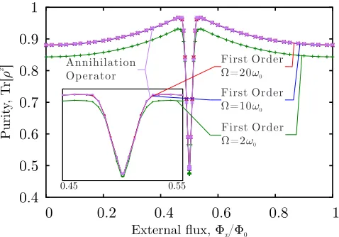
FIG. 1. (colour online) To quantify the importance of cutoff frequency, Ω, in the first order master equation Eq. (26), we show Tr

ρ2

as a function of external flux ˆΦx for the steady

state solution to the master equation forξ =ω0/Ω equal to

0 (Ω =∞), 0.05 (Ω = 20ω0), 0.1 (Ω = 10ω0) and 0.5 (Ω =

2ω0). We see that Ω =∞and Ω = 20ω0are indestinguishable

whilst near the dip at Φx= 0.5Φ0 there are small differences

at Ω = 10ω0. While the functional form is similar the effect

of cut-off frequency is significant for Ω = 2ω0. Note, circuit

parameters areC = 5×10−15

F,L = 3×10−10

H and Ic ≈

3µA. The sharp dip at Φx = Φ0/2 is due to the fact that

the SQUID’s potential becomes a double well and the ground energy eignstate is a Schr¨odinger cat (i.e. a macroscopically distinct superposition of states). Decoherence of this state produces a statistical mixture of states equally localised in each well - as there is a 50% chance of being in either well Tr

ρ2

= 0.5 at Φx = Φ0/2. As we move away from this

bias point the ground state rapidly loses its Schr¨odinger cat structure and so decoherence is less significant at these values. The width of this dip is related to the the barrier hight and can be changed by altering circuit parameters.

In this work, we have chosen reasonable SQUID

pa-rameters values ofC= 5×10−15_{F andL= 3×10}−10_H

are used in all caluculations together with a Josephson coupling energy20 _{of ~ν = I}

cΦ0/2π = 9.99×10−22J,

where Φ0=h/2eis the flux quantum andIc is the criti-cal current of the weak link (hereIc ≈3µA). The exter-nal environment is defined by the parameters γ, Ω, ~_ν, and Φxwhere the damping rateγdetermines the rate of loss in the system. Treating the environment as a cavity of harmonic oscillator modes, this loss is directly pro-portional to the cavity quality factor Qc = 2πωc/γ for cavity frequencyωc. This quality factor can range from Qc ∼ 102 to Qc ∼ 106 or higher49,50. The cutoff fre-quency, Ω, defines the peak frequency of the bath’s spec-tral density which has a similar form to the impedance in Josephson circuits51,52_{. The results shown in Fig. 1}

might lead us to conclude that for a cut off frequency of Ω = 10ω0 (ξ = 0.1) and higher (lower) that the usual

choice of a Lindblad proportional to the annihilation op-erator is a good one. In the next section we show that this conclusion is incorrect.

VI. SECOND ORDER APPROXIMATION

Although for systems of this type it is often assumed to be adequate, truncation at first order of series (Eq. (23)) may not always suffice and higher order terms in τ (or equivalently ω0/Ω) may be important; consideration of

a second order expression will help to justify that. It is also important to explore the impact of higher order terms as higher order models may differ quantitatively, if not qualitatively, to the first order model. Expanding Eq. (23) to second order inτ we obtain:

X

n n!

ΩnAn≈Φˆ− ˆ Q ΩC−

ω2

Ω2

ˆ

Φ +2π~νL Φ0

sin

2π Φ0

( ˆΦ + Φx)

(28) where the external flux dependence, originating from the non-linear SQUID potential, can be seen to enter the dissipator for the first time. Substituting (28) into (22) then allows (13) to be rewritten as:

dρS dt =−

i

~[ ˆHS, ρS(t)] + iγΩC

~

renormalisesL

z }| {

1−ω 2 0

Ω2

[ ˆΦ2, ρS(t)]]−

1st

order dissipation

z }| {

1

ΩC[ ˆΦ,{Q, ρˆ S(t)}]−

2nd

order dissipation

z }| {

2π~_νL Φ0 ω2 0 Ω2 ˆ Φ, sin 2π Φ0

( ˆΦ + Φx)

, ρS(t)

!

−γω₂0_~C

1−ω 2 0

Ω2

[ ˆΦ,[ ˆΦ, ρS(t)]]

| {z }

1st

and 2nd

order noise

−_Ω1_C[ ˆΦ,[ ˆQ, ρS(t)]]

| {z }

1st

order in cutoff

−2π_Φ~νL 0 ω2 0 Ω2 ˆ Φ, sin 2π Φ0

( ˆΦ + Φx)

, ρS(t)

| {z }

2nd

order cutoff

!

(29)

where once again HˆS consists of the true in-ductance of the SQUID ring after second or-der renormalisation is accounted for, i.e. λ =

2γΩ1− ω

2 0 Ω2 /ω2 0

1 + 2_ωγ2Ω 0

1−ω

2 0

Ω2

.

External ux, /x 0

³

at

min

0.6 0.65 0.7 0.75 0.8 0.85 0.9 0.95 1

0 0.2 0.4 0.6 0.8 1

=50!0

=10!0

=2!0

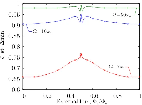
FIG. 2. (colour online) A plot of the second order weighting parameterζ that minimises the difference between first and second order master equations as a function of external flux. ∆min is defined to be the minimal difference in steady state

purity between first and second order models, for system pa-rameters Ω,Φx. We see that theζ that is minimally invasive

is a non-linear function of external flux. For high cut off fre-quency this is approximated byζ= 1−ω0/Ω (where we note

that this approximation is less good around Φx= Φ0/2).

and it is of interest to observe the form that the Lindblad operators now take. Two Lindblads ˆL1=α1Φ +ˆ ǫ1Qˆ and

ˆ

L2 = α2Φ +ˆ ǫ2sin

2π

Φ0( ˆΦ + Φx)

are needed; the first is an annihilator while the second represents a correction to the environmental interactions and is a function of the external flux control parameter Φx.

There is some flexibility to the manner in which the fifth term in Eq. (29) may be split between the two Lindblads, ˆL1 and ˆL2. The weighting of this

split, with respect to first and second order contri-butions, is characterised in this work by the weight-ing parameter ζ and is allocated in such a way that −(1−ζ)γω0C

2~

1−ω

2 0

Ω2

[ ˆΦ,[ ˆΦ, ρS(t)]] contributes to ˆL1

and −ζγω0C

2~

1−ω

2 0

Ω2

[ ˆΦ,[ ˆΦ, ρS(t)]] contributes to ˆL2.

Usually a ‘minimally invasive’ approach is taken to en-sure that first order terms remain dominant and the extra term needed for ˆL2 is as small as possible. In Fig. 2 we

show the value ofζ which finds the minimum difference ∆minin steady state purity between the first and second

order master equations. For most systems this would be expected to be constant value but for the SQUID ring it is non-linearly dependent on external flux. This is not as surprising as it might first seem as SQUID rings are known to effect externally coupled oscillators (tank-circuits) in a non-linear way and the environment is con-sidered as an infinite bath of such oscillators. As a result we expect that the modelling process should also yield re-sults that are also non-linearly dependent on the external flux.

It is therefore the case that the Lindblad form of the master equation expressed to second order should contain a correction that is dependent on external flux and cutoff frequency – ζ(Ω,Φx). These and some other subtleties will be explored in a followup work. We see that for high cut-off frequency that choosing ζ = 1−ω0/Ω =

1−ξ is a good approximation to a minimally invasive master equation (especially away from Φx= 0.5). With this choice, the Lindblad operator ˆL1 again approaches

the annihilation operator in the high cut off limit, where ξ → 0. In the remainder of this work we will thefore make the approximation thatζ= 1−ω0/Ω. Within this

model, frequency shifts are still accounted for, as they are enclosed within the third term in Eq. (29). The second order equation also possesses a second frequency shift. It must be expected that higher order approximations in ω0/Ω will introduce additional Lindblad operators and

additional frequency renormalisation, this again will be investigated in future work.

If the additional terms, required to bring the equation into Lindblad form are included in Eq. (29), one obtains:

dρ dt =−

i

~[ ˆH, ρ] + 1 2

X

j

[ ˆLj, ρLˆ†j] + [ ˆLjρ,Lˆ†j]

ˆ

H = ˆHS2+

~_γ

2

ˆ

XPˆ+ ˆPXˆ+

r

βξν ΩXˆsin

r

βω0

ν Xˆ + 2π Φx Φ0

!

ˆ L1=γ

1 2

" p

(1−ξ) (1−ξ2_{) ˆX+}

i−ξ₂ s

1

(1−ξ) (1−ξ2₎Pˆ #

ˆ L2=γ

1 2

" p

ξ(1−ξ2_{) ˆX+} s

ξ (1−ξ2₎

i−ξ₂ r

β ν ω0

sin

r

βω0

ν Xˆ + 2π Φx Φ0

!#

(30)

where here we introduced the parameterβ= 2πLIc/Φ0,

related to the critical current Ic = 2π~ν/Φ0, which is

0.4 0.5 0.6 0.7 0.8 0.9 1

0 0.2 0.4 0.6 0.8 1

st

1 Order

=10!0

nd

2 Order

=10!0

st

1 Order

=2!0

2

Purit

y, T

r[

½

]

External ux, /x 0

FIG. 3. (colour online) The purity Tr{ρ2

(t)}of the steady state solutions of the first order, Eq. (26), and second or-der Eq. (30), Lindblad master equations. In this figure we see evidence that the order of truncation has a bigger effect on the steady state purity than one might expect when compared to that of decreasing cut-off frequency.

teretic (β >1) from non-hysteretic behaviour (β≤1).

In Fig. 3 we compare the purity Tr{ρ2_{(t)}of the steady}

state solutions of the first order, Eq. (26), and second or-der Eq. (30), Linblad master equations for a cut-off fre-quency of Ω = 10ω0. We have also included for

compari-son the first order master equation steady state purity for Ω = 2ω0. In Fig. 1, for a cut-off frequency of Ω = 10ω0,

we concluded that there was little difference between the steady state solution to the first order corrected mas-ter equation and one that just assumed an annihilation operator as a Lindblad. In Fig. 3, for the same value of cut-off frequency, we observe that the steady state purity is much lower and changes slightly in functional form in the second order model. This indicates that neither the annihilation operator nor first order Lindblads are suffi-cient to quantitatively model the effects of decoherence on the SQUID ring.

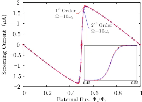
The difference between first and second order models is less obvious when considering the expectation value of observables, such as screening current, as shown in Fig. 4. This suggests that device characterisation based solely on simple expectation values of observables such a flux may not be sufficient and a more rigorous analysis of decoherence times,T1andT2, as functions of external

flux is necessary in order to produce a good phenomenol-ogy. Such an approach may be used to parameterise the master equation framework presented in this work and to assess its effectiveness in modelling decoherence processes on Josephson junction based devices.

-2 -1.5 -1 -0.5 0 0.5

1 1.5

2

0 0.2 0.4 0.6 0.8 1

0.45 0.55

External ux, /x 0

Screening Curren

t

(

¹

A)

st 1 Order

=10!0

nd 2 Order

=10!0

FIG. 4. (colour online) A plot of the expectation value of screening current,DΦˆ/LEas a function of external flux for first order (red) and second order (blue) models at a bath cut-off frequency of Ω = 10ω0. Despite the two models differing

quite largely in terms of steady state purity, the expectation values of observables remain very similar.

VII. CONCLUSIONS

The necessity to consider stronger environmental cou-pling than might be admitted in lowest order Born Ap-proximation, or the effects of a finite bath cut-off fre-quency, or of a device operating at low temperature, sug-gest that the standard Born-Markov development of a Master Equation will need to be extended. The most obvious way to do this is through a small parameter ex-pansion, such as the Born series or, as here, by extending the large cut-off limit by developing the model as a series in the small parameter ω0/Ω, or similarly by extending

a zero temperature limit. We have chosen, here, perhaps the simplest case (that of a finite cut-off), in the certain knowledge that whatever difficulties one finds are very likely to appear in all others such attempts.

The most obvious consequence of the present anay-sis is that the correction obtained by including second order terms (in ω0/Ω) in the Master Equation is not

an insignificant one, leading to steady-state impurities 1−P(ρ) which are twice those predicted by using a first order model. More subtle is the appearance of the ex-ternal flux Φx entering the Master Equation, not only in the Hamiltonian terms, but also in the second order Lindblad. Indeed with capacitive coupling the external flux is likely to appear in Lindblads at all orders. As the Josephson coupling energy dictates the height of the potential well, and therefore the tunnelling probability, SQUIDs are (notoriously) sensitive to external magnetic fields and so it is reasonable to expect a strong external flux dependence19,20,53_{; Eq. (30) shows such a}

systems with Lindbladian dissipation, control parameters such as Φxwill only enter through the Hamiltonian (see, e.g., [54]), it is evident from the form of Eq. 21 that Φx can play an important role in dissipation. That the dissi-pator will in general a function of control parameters has been pointed out previously55_{, the current analysis shows}

they may not all enter at the same order. Furthermore, we have shown that the second order correction to the master equation has a surprisingly large effect. Hence, an understanding of this phenomenon and the role of Φxwill be of importance to those working on Josephson junction based devices especially for emerging quantum technologies.

Recent analysis of the Quantum Brownian Motion (QBM) system indicates that both regular and anoma-lous diffusion parameters show a logarithmic divergence on bath cut-off frequency Ω, implying a finite cut-off. It thus makes sense to consider a series solution, to differ-ent orders ofω0/Ω, if only to check that the common first

order truncation is accurate. It is not surprising that, as with QBM, it is necessary to add extra terms in order to bring the master equation into Lindblad form and so avoid unphysical system development. However, in our second order approximation, the extra term needed to complete the first order Lindblad ˆL1 is of a lower order

than the terms which make up the second order Lind-blad ˆL2. This makes the ‘minimally invasive’ argument

a difficult one to sustain and so we appear to be left with the choice of abandoning hierarchical checks, reworking a new standard method, or abandoning the Lindblad form for systems such as these. None of which is attractive.

With the exception of a quadratic constraining poten-tial, which is simple because the position operator (Φ here) links only neighbouring states of fixed energy dif-ference ω0, all other systems are likely to run into the

same difficulties we have here.

ACKNOWLEDGMENTS

MJE would like to thank Kae Nemoto and SNAD would like to thank Todd Tilma for the generous hos-pitality, valuable discussions, and support whilst visiting them in Tokyo. SNAD and MJE would like to thank Michael Hanks and Jason Ralph for many valuable, and enjoyable, discussions. MJE, KNB and VMD would like to thank the DSTL for their support through the grant

Engineering for Quantum Reliability. This paper recog-nises the use of the ‘Hydra’ High Performance System at Loughborough University.

∗ _{m.j.everitt@lboro.ac.uk} 1

J. P. Dowling and G. J. Milburn, Philosophical transac-tions. Series A, Mathematical, physical, and engineering sciences361, 1655 (2003).

2

S. Boixo, T. F. Rønnow, S. V. Isakov, Z. Wang, D. Wecker, D. a. Lidar, J. M. Martinis, and M. Troyer, Nature Physics 10, 218 (2014).

3

J. Clarke and I. Braginski, Alex, eds.,The SQUID Hand-book, Vol. 1 (Wiley-VCH, 2004) pp. 127–170.

4

B. Ruggiero, V. Corato, C. Granata, L. Longobardi, S. Rombetto, and P. Silvestrini, Physical Review B 67, 132504 (2003).

5

K. Ogunyanda, W. Fritz, and R. van Zyl, Journal of En-gineering, Design and Technology13, 298 (2015).

6

U. Weiss,Quantum Dissipative Systems (World Scientific Publishing, 1999).

7

E. Joos, H. D. Zeh, C. Kiefer, D. Guilini, J. Kupsch, and O. Stamatescu, I, Decoherence and the Appearance of a Classical World in Quantum Theory, 2nd ed. (Springer, 2003).

8

J. P. Santos and F. L. Semiao, Physical Review A - Atomic, Molecular, and Optical Physics89, 022128 (2014).

9

G. Lindblad, Communications in Mathematical Physics 48, 119 (1976).

10

C. W. Gardiner,Quantum Noise (Springer-Verlag, Berlin, 1991).

11

H. Breuer and F. Petruccione,The Theory of Open Quan-tum Systems (Oxford University Press, 2002).

12

M. Schlosshauer, Decoherence: And the Quantum-To-Classical Transition (Springer, 2007).

13

W. Munro and C. Gardiner, Physical Review A53, 2633 (1996).

14

S. Gao, Physical Review Letters79, 3101 (1997).

15

C. H. Fleming, A. Roura, and B. L. Hu, Annals of Physics 326, 1207 (2011).

16

P. Massignan, A. Lampo, J. Wehr, and M. Lewenstein, Physical Review A - Atomic, Molecular, and Optical Physics91, 033627 (2015).

17

G. Burkard, Physical Review B - Condensed Matter and Materials Physics71, 1 (2005).

18

C. Cohen-Tannoudji, B. Diu, and F. Laloe,Quantum Me-chanics (Wiley-VCH, 2005).

19

M. J. Everitt, T. D. Clark, P. Stiffell, H. Prance, R. J. Prance, a. Vourdas, and J. Ralph, Phys. Rev. B64, 184517 (2001).

20

M. Everitt, P. Stiffell, T. Clark, a. Vourdas, J. Ralph, H. Prance, and R. Prance, Physical Review B63, 144530 (2001).

21

T. Clark, J. Diggins, J. Ralph, M. Everitt, R. Prance, H. Prance, R. Whiteman, a. Widom, and Y. Srivastava, Annals of Physics268, 5821 (1998).

22

F. Helmer, M. Mariantoni, E. Solano, and F. Marquardt, Physical Review A79, 052115 (2009).

23

G. Romero, J. J. Garc´ıa-Ripoll, and E. Solano, Physical Review Letters102, 173602 (2009).

24

P. B. Stiffell, M. J. Everitt, T. D. Clark, C. J. Harland, and J. F. Ralph, Physical Review B - Condensed Matter and Materials Physics72, 014508 (2005).

25

Y. Hu, G. Q. Ge, S. Chen, X. F. Yang, and Y. L. Chen, Physical Review A - Atomic, Molecular, and Op-tical Physics84, 012329 (2011).

26

27

A. Caldeira and A. Leggett, Physica A: Statistical Mechan-ics and its Applications121, 587 (1983).

28

C. H. Chou, B. L. Hu, and T. Yu, Physica A: Sta-tistical Mechanics and its Applications387, 432 (2008), 0708.0882.

29

L. Di´osi, Europhysics Letters (EPL)22, 1 (1993).

30

J. J. Halliwell and T. Yu, Physical Review D 53, 2012 (1996).

31

B. L. Hu, J. P. Paz, and Y. Zhang, “Quantum Brownian motion in a general environment: Exact master equation with nonlocal dissipation and colored noise,” (1992).

32

W. G. Unruh and W. H. Zurek, Physical Review D 40, 1071 (1989).

33

G. S. Agarwal, Physical Review A4, 739 (1971).

34

R. J. Prance, T. P. Spiller, H. Prance, T. D. Clark, J. Ralph, A. Clippingdale, Y. Srivastava, and A. Widom, Il Nuovo Cimento B Series 11106, 431 (1991).

35

P. R. J. Diggins J, Ralph J F, Spiller T P, Clark T D, Prance H, Physical Review E49, 1854 (1994).

36

T. P. Spiller, D. A. Poulton, T. D. Clark, R. J. Prance, and H. Prance, International Journal of Modern Physics B 5, 1437 (1991).

37

H. M. Wiseman and W. J. Munro, Phys. Rev. Lett. 80, 5702 (1998).

38

M. J. Everitt, W. J. Munro, and T. P. Spiller, Physical Review A - Atomic, Molecular, and Optical Physics 79, 032328 (2009).

39

M. J. Everitt, New Journal of Physics 11 (2009), 10.1088/1367-2630/11/1/013014.

40

A. Montina and F. T. Arecchi, Physical Review Letters 100, 120401 (2008).

41

A. Kapulkin and A. K. Pattanayak, Physical Review Let-ters101, 074101 (2008).

42

H. Li, J. Shao, and S. Wang, Physical Review E - Statisti-cal, Nonlinear, and Soft Matter Physics84, 051112 (2011), 1205.4616.

43

N. Bogoliubov, Journal of Physics9, 23 (1947).

44

M. J. Everitt, T. P. Spiller, G. J. Milburn, R. D. Wilson, and A. M. Zagoskin, Frontiers in ICT1, 1 (2014).

45

L. Viola, R. Onofrio, and T. Calarco, Measurement9601, 7 (1997).

46

M. A. Nielsen and I. L. Chuang, Quantum Dynami-cal Semigroups and Applications (Cambridge University Press, Cambridge, 2000).

47

J. Dajka and J. Luczka, Physical Review B - Condensed Matter and Materials Physics80, 174529 (2009).

48

H. Nakano, H. Tanaka, S. Saito, K. Semba, H. Takayanagi, and M. Ueda, Science And Technology , 15 (2004).

49

Y. X. Liu, L. F. Wei, and F. Nori, Physical Review A72, 033818 (2005).

50

J. D. Whittaker, F. C. S. Da Silva, M. S. Allman, F. Lecocq, K. Cicak, A. J. Sirois, J. D. Teufel, J. Aumen-tado, and R. W. Simmonds, Physical Review B - Con-densed Matter and Materials Physics90, 024513 (2014).

51

Y. Makhlin, G. Sch¨on, and A. Shnirman, Chemical Physics296, 315 (2004).

52

A. Shnirman, Y. Makhlin, and G. Sch¨on, Physica Scripta T102, 147 (2002).

53

M. J. Everitt, T. D. Clark, P. B. Stiffell, J. F. Ralph, and C. J. Harland, Physical Review B - Condensed Matter and Materials Physics72, 094509 (2005).

54

P. Rooney, A. M. Bloch, and C. Rangan, arXiv:1602.06353v1 (2016).

55