Early influences on saving behaviour: Analysis of British panel data

Early influences on saving behaviour: Analysis of British panel data

Sarah Brown

⇑

, Karl Taylor

Department of Economics, University of Sheffield, 9 Mappin Street, Sheffield S1 4DT, United Kingdom

a r t i c l e i n f o

Article history:

Received 24 September 2014 Accepted 14 September 2015 Available online 21 September 2015

JEL classification: D12

D14

Keywords: Household finances Panel data Saving

a b s t r a c t

Using data from the British Household Panel Survey and Understanding Society, we examine the saving behaviour of individuals over time. Initially, we explore the determinants of the saving behaviour of chil-dren aged 11–15. Our findings suggest that parental allowances/pocket money (earnings from part-time work) lower (increase) the probability that a child saves. There is also evidence that the financial expec-tations of the head of household have an influence on their offspring’s saving behaviour, where children of optimistic parents have a lower probability of saving by approximately 2 percentage points. However, there is no evidence of an intergenerational correlation in savings behaviour: the saving behaviour of par-ents appears to have no bearing on the saving decisions of their offspring. We then go on to explore the implications of the saving behaviour of children for their savings decisions in later life, specifically when observed in early adulthood. We find that having saved as a child has a large positive influence both on the probability of saving on a monthly basis and on the amount saved as an adult. This finding is robust to alternative empirical strategies including IV analysis where the most conservative estimates show that having saved as a child increases the probability of saving during adulthood by 12 percentage points. Ó2015 The Authors. Published by Elsevier B.V. This is an open access article under the CC BY license (http://

creativecommons.org/licenses/by/4.0/).

1. Introduction and background

Household saving has attracted considerable interest in the eco-nomics literature with particular focus on the various motivations behind saving behaviour, which are arguably complex and interre-lated. Browning and Lusardi (1996) present a comprehensive review of household saving from both an empirical and a theoret-ical perspective in which they discuss motivations for savings focusing on those listed by Keynes (1936). Such motivations include: precautionary saving where households hold a contin-gency fund in case of adverse future events; to smooth income and consumption over the life cycle; and the inter-temporal substi-tution motive whereby households benefit from accumulating interest on savings. Clearly, motives for saving will differ across households as well as over time for a given household. Such motives are likely to be interrelated and, indeed, complementary. For example, a household which saves to accumulate interest from savings will also hold a fund to be used should unforeseen adverse events occur. Regardless of the motivations behind saving beha-viour, a commonly held view is that individuals and households are not saving enough in the context of both short-term saving

as well as long-term saving for retirement (see, for example, Crossley et al., 2012). We contribute to the existing empirical literature on saving by exploring the implications of saving beha-viour at the early stages of the life cycle, from childhood through to early adulthood, which has attracted very little interest in the economics literature.1

Although most children do not hold financial assets, it is appar-ent that children may face saving decisions albeit in the context of saving, for example, for a toy or for the latest mobile phone as opposed to large scale saving decisions, such as a house purchase. Evidence from the economic psychology literature suggests that children are capable of saving. For example,Otto et al. (2006)adopt an experimental approach to explore children’s use of saving strate-gies in the context of saving for a toy when faced with income uncertainty. The results based on a sample of 42 children indicate that children aged between 9 and 12 are able to formally manage their money, with children aged 12 frequently making ‘bank’ deposits as a means to avoid the temptation to spend tokens on, for example, sweets. In Section2, we contribute to this embryonic

http://dx.doi.org/10.1016/j.jbankfin.2015.09.011 0378-4266/Ó2015 The Authors. Published by Elsevier B.V.

This is an open access article under the CC BY license (http://creativecommons.org/licenses/by/4.0/). ⇑ Corresponding author.

1

The shortage of existing research in this area may reflect issues with data availability. In particular, there is a distinct lack of large scale representative surveys which include information on children’s saving behaviour. For example, in our analysis, we require information on saving behaviour as a child, parental saving behaviour when the respondent was a child and saving behaviour in early adulthood.

Contents lists available atScienceDirect

Journal of Banking & Finance

literature by exploring the determinants of children’s saving beha-viour using data drawn from a large scale nationally representative survey. We focus on whether an intergenerational link exists between the saving behaviour of parents and their children.

One might conjecture that an intergenerational link exists between the attitudes towards finances between parents and their children as parents may seek to equip their children with particu-lar values and life skills. The financial literacy of young adults and the role of financial education in preparing children and young adults for entry into a complex economic and financial environ-ment is a topical issue (seeLusardi and Mitchell, 2014, for a recent review), yet there has been limited discussion of the intergenera-tional relationship between such skills and attitudes. Such an asso-ciation may reflect an intergenerational link between both cognitive skills in terms of financial literacy as well as non cogni-tive skills such as attitudes towards finances and taking risk. As argued byLusardi and Mitchell (2007), p. 213, ‘savings decisions are complex, requiring consumers to possess substantial economic knowledge and information.’ It may be the case, therefore, that parents who possess a certain degree of financial literacy may seek to impart such skills to their offspring in order to equip them with financial management skills for the future.

Hence, children and young adults may acquire attitudes towards finances from their parents. For example, Mandell

(2008)reports that parents are the key source of financial

informa-tion for students at high school.Grinstein-Weiss et al. (2011), who explore a sample of low and moderate income households, find that adults who received relatively high levels of money-management education from their parents during their childhood had lower credit card debt and higher credit scores as adults. Such findings tie in with the recent education literature (seeBlack and Devereux, 2011, for a comprehensive survey), which has docu-mented the existence of strong positive intergenerational associa-tion in educaassocia-tional attainment, which itself has clear implicaassocia-tions for future income and wealth generation.

A related strand of the literature on intergenerational aspects of economic and financial attitudes has focused on estimating the intergenerational elasticity of wealth between parents and their adult children. For example,Charles and Hurst (2003)estimate this age-adjusted elasticity at 0.37 prior to the transfer of bequests using data from the U.S. Panel Study of Income Dynamics (PSID). Lifetime income and asset ownership are found to be key determi-nants of the wealth elasticity, with shared risk preferences explain-ing a relatively small portion of the intergenerational wealth elasticity. Thus, the findings in the existing literature support a sizeable intergenerational correlation of wealth.

In a seminal contribution,Becker (1993)argues that children are heavily influenced by the attitudes and behaviour of their par-ents, with childhood experiences during the formative early years serving to shape individuals’ preferences. Furthermore, as argued

by Knowles and Postlewaite (2004), parents invest considerable

amounts of time, effort and money in order to influence the prefer-ences of their children. Using U.S. data,Knowles and Postlewaite

(2004) find that parents’ saving behaviour influences the saving

behaviour of their adult offspring. They present a life-cycle model in which intergenerational savings correlations can be interpreted as intergenerational discount-factor correlations. They use data from the U.S. PSID to estimate family savings effects, which are found to be economically and statistically significant. In the con-text of their model, family effects can be linked to factors such as patience or self-control (see, for example, seminal contributions

byThaler and Shefrin, 1981, who present an intertemporal choice

model of self-control with the individual being both a ‘farsighted

plannerand a myopic doer’ andBecker and Mulligan, 1997, who

analyse the endogenous determination of time preference). With respect to skills and attitudes towards financial planning,

Ameriks et al. (2003)present evidence supporting the role of

dif-ferences in planning in influencing the propensity to save and sav-ing patterns. Such findings suggest that intergenerational transmission of preferences and attitudes may lead to intergener-ational correlation in financial decision-making such as saving behaviour.

More recently, Cronqvist and Siegel (2015), using data on Swedish twins aged between 20 and 65, explore the origins of saving behaviour. Their findings suggest that genetic differences explain approximately 33 percent of the variation in propensity to save across individuals. Parenting is found to influence the variation in savings rates for younger individuals, but the effect diminishes over time. Environmental factors during the individual’s childhood such as parental wealth are found to moderate the genetic effects. Having explored the determinants of saving behaviour during childhood, in Section3we investigate the influence of saving beha-viour as a child on saving decisions in early adulthood. This may have further implications for financial behaviour and decision-making at later stages of the life cycle. It is apparent that saving decisions during childhood may influence attitudes towards finances at later stages of the life cycle and, hence, have implica-tions for saving behaviour observed during adulthood. Indeed, our empirical findings, based on panel data which follows individ-uals from childhood into adulthood, suggest that having saved as a child has relatively large positive effects on both the probability of saving and the amount saved as an adult, a finding which is robust to a number of alternative empirical strategies – with the most conservative estimates at 12 and 14 percentage points respectively.

2. Saving behaviour during childhood

2.1. Data and methodology

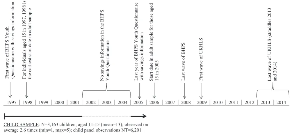
We analyse the British Household Panel Survey (BHPS), a survey conducted by the Institute for Social and Economic Research com-prising approximately 10,000 annual individual interviews from 1991 to 2008.2_{Since 1994, children aged 11–15 completed a short}

interview for the BHPS Youth Questionnaire. On reaching age 16, they complete the standard adult questionnaire, which allows us to follow the individuals into adulthood (see Section3for further details andFig. 1 which provides an event-timeline depicting the years of observation for the empirical strategy). In the BHPS Youth Questionnaire for years 1997–2001 and 2005, the children were asked ‘what do you usually do with your money?’ The possible responses were:save to buy things;save and not spend; andspend

immediately. The responses thus provide information relating to

the saving behaviour of children: 43% of children save to buy things; 35% save and not spend; and 22% spend immediately. Pooling the BHPS Youth Questionnaire for years 1997–2001 and 2005, when the information on childhood saving behaviour was elicited, we obtain an unbalanced panel of data with 6201 observations consist-ing of 3163 children, who are observed in the panel, on average, 3 times. We are able to match the responses to the BHPS Youth Questionnaire with that of the adult questionnaires in order to link information relating to children and their parents.

We focus on exploring the determinants of the probability that children save rather than spend their money immediately via a random effects binary probit framework as follows:

SCit¼1½X01itbþ/logðS P itÞ þEXP

P0

it

c

þ

a

iþ

e

it>0 ð1Þ

2

where there arei =1,. . .Nchildren, andt= 1,. . .Ttime periods,SC itis an indicator variable for whether the child saves. The individual specific unobservable effect in the error term is denoted by

ai

, i.e. a random effect

ai

IIDð0;

r

2

aÞ, and

e

it is a white noise error term, i.e.

_e

itIIDð0;

r

2itÞ. This specification allows for correlation between the error terms of children over time, i.e.

q

1¼

r

2a=ð

r

2aþ

r

2eÞ, which

represents the proportion of the total unexplained variance in the dependent variable contributed by the panel level variance compo-nents. If the panel component of the data is important then we would expect

q

1–0, where the magnitude of the parameter indi-cates the extent of the unobservable intra-personal correlation in children’s saving behaviour over time.

The control variables in_X1it include the allowance received by the child in the previous week,3_{the pay received by the child from}

part-time work in the previous week, and additional child and household characteristics. The information on allowances is elicited from the following question: ‘How much money did you receive last week to spend on yourself? Please include pocket money and any allow-ance you get. But if you have a job, do not include money you earned.’ Information relating to hours worked for pay and the money received from that work is derived from the following question

asked to children: ‘Last week, how many hours did you spend doing work for pay?’4They were also asked: ‘How much money did you earn last week? Do not include pocket money or allowances.’ It is apparent that the responses to these questions could potentially cover earn-ings from both formal and informal employment. Indeed, children in the UK are legally allowed to work from the age of 13, with certain exceptions that allow working at a younger age, such as work in tele-vision, the theatre or modelling, which requires a performance licence. Hence, reported hours of work below the age of 13 could relate to this specific type of work or could reflect informal work, possibly carried out at home.5

Additional characteristics of the child included inX1it are as follows: gender; a quadratic in age; whether the child is the natural child of his/her parents; a binary indicator for whether the child does not have a computer at home; in terms of educa-tional aspirations, we control for whether the individual intends to go to college or sixth form after the compulsory schooling age of 16. Additionally, we control for household/parent characteristics inX1itspecifically: equivalized yearly household income (based on 1997 1998 1999 2000 2001 2002 2003 2004 2005 2006 2007 2008 2009 2010 2011 2012 2013 2014

F

ir

st

wav

e

of

BH

PS

Youth

Qu

es

tionnaire

w

ith

sa

v

ing

s

inf

or

m

at

io

n

For

indi

v

idual

s

ag

ed

15

in

1997

,

1998

is

the

ea

rl

ie

st

s

ta

rt

d

at

ei

n

adul

ts

ample

No s

av

ing

s

in

form

at

ion

in

th

e

B

HP

S

Youth

Qu

e

st

ionn

air

e

La

st

ye

a

r

o

f

BH

PS

Youth

Q

u

e

st

ionna

ire

with

sav

in

gs

in

fo

rm

at

ion

S

tar

t

da

te

in

a

d

ul

t

sample

for

those

ag

ed

15

in

2005

L

as

tw

a

ve

of

B

H

PS

Firs

t

w

av

e

o

f

U

K

H

LS

La

st

wa

ve

of

U

K

H

LS

(stra

ddles

201

3

a

n

d

2014)

CHILD SAMPLE: N=3,163 children; aged 11-15 (mean=13); observed on average 2.6 times (min=1, max=5); child panel observations NT=6,201

[image:3.595.48.547.69.301.2]

ADULT SAMPLE: N=2,526 adults tracked from childhood; aged 16-30 (mean=20); observed on average 3.4 times (min=1, max=8); adult panel observations NT=7,078

Fig. 1.Event timeline.

3

There are a small number of studies in the economic psychology literature exploring the provision of pocket money to children. For example,Furnham (2001) explores parental attitudes towards pocket money amongst a sample of 300 British parents. Approximately three-quarters of the sample believed that children should be encouraged to save pocket money or financial gifts. Such findings support the notion that the provision of pocket money represents a kind of ‘economic education’ (see, Barnet-Verzat and Wolff (2002), for a concise survey of this area).Barnet-Verzat and Wolff (2002) explore the motives behind intergenerational financial transfers focusing on pocket money and discuss three main motives in the economics literature for transfers from parents to children: ‘altruism, exchange and preference shaping.’ Their econometric study of 5300 families in France indicates heterogeneity in parental motives to give pocket money.

4

In the UK, there are legal restrictions imposed on child employment (for further details seehttp://www.direct.gov.uk/en/Parents/ParentsRights/DG_4002945). In par-ticular, during school term time children may work a maximum of 12 h per week, whereas during school holidays, 13–14 (15–16) year olds may work a maximum of 25 (35) hours per week. The interviews for the BHPS took place in January, February, March, April, May, September, October, November and December. Since the interviews did not take place in the main school holiday period (July and August), we treat 12 h per week as the upper limit on hours worked. We, therefore, omit 2% of the sample of children who report weekly hours of work in excess of 12 h.

5

the McClements equivalence scale before housing costs);6_the

high-est level of educational attainment of the parent distinguishing between degree, further education, A level, O level (GCSE), with no education as the omitted category;7_{housing tenure to proxy}

house-hold wealth, i.e. owning the home without a mortgage, owning the home with a mortgage and renting from the council (the reference category is renting from a housing association, or an employer, or privately rented); the number of adults in the household; the number of children in the household; a binary indicator for a single parent household; whether either parent talks to the child about issues which are important on a daily basis (the idea here is that this might capture the importance of verbal directives); year controls; and region controls.

To ascertain whether an intergenerational link exists in saving behaviour, we include the monthly amount saved by the child’s parent, SP

it, in the set of explanatory variables. This is based on responses to the following question: ‘Do you save any amount of your income, for example, by putting something away now and then in a bank, building society, or Post Office account other than to meet regular bills? About how much, on average, do you manage to save a month?’ Hence, it relates to ‘active’ saving. As well as providing information on parental saving, the BHPS includes information on the financial expectations of adults in the household. To be specific, adult members of the household were asked: ‘Looking ahead, how do you think you yourself will be financially a year from now, will you be: better than now; worse than now; or about the same’? Hence, we also explore whether parental financial expecta-tions influence the saving behaviour of their offspring by including these controls in the vector EXPPit, specifically whether future finances are expected to improve (optimistic) or whether no change in finances is expected, with future finances expected to get worse (pessimistic) comprising the reference category.8

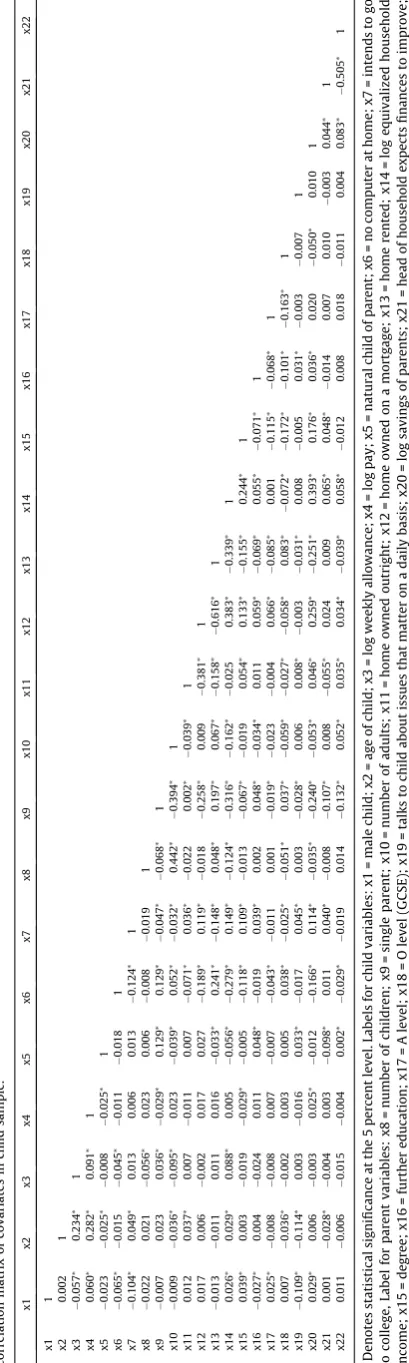
Sum-mary statistics of the above variables are presented inTable 1and a correlation matrix of the covariates used in the analysis is given

inTable A1in the appendix, where clearly the degree of correlation

is relatively low amongst the control variables even where statisti-cally significant.9

2.2. Results

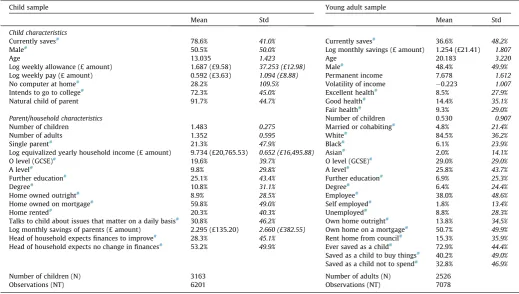
In the first column ofTable 2we present the findings from the random effects probit analysis, i.e. from estimating Eq.(1), where standard errors and marginal effects are reported.10_{Clearly, over}

time the unobserved individual child heterogeneity of the panel is important both in terms of magnitude and statistical significance in explaining the residual variance, as can be seen by the estimated

q

1parameter. The results indicate that the child’s allowance is neg-atively associated with the probability that the child saves. The mag-nitude of the effect of a 1 percent increase in the child’s allowance is associated with a decrease in the probability that the child saves by 2.2 percentage points. In contrast, the weekly pay that the child receives from part-time work is positively associated with the

probability of saving, thus, indicating a distinct difference in the influence of these two different sources of children’s income on their saving behaviour.11

The intergenerational coefficient on the amount of monthly sav-ings of the parents, i.e./, is positive but statistically insignificant.12

Hence, it would appear that the saving behaviour of parents does not influence the saving decision of their offspring, which may reflect the possibility that parents do not share information regarding such household financial matters with their children. This could be a con-sequence of parental savings being quite passive: for example, if there is a regular bank transfer from a current account into a savings account, then arguably this is not an observed behaviour but rather an automated financial transaction. It is more conceivable that those parents who explicitly discuss this action or, indeed, the decision to carry out this action with their children might pass on a saving men-tality.13 In contrast, spending may be regarded as overt in that it potentially manifests itself in terms of, for example, new clothes or a new car. If it is the case that saving tends to be passive whilst spending is overt, parental behaviour may serve to send signals that are contrary to the message of saving and planning that a parent would ideally like their children to learn.14_{In contrast, with respect}

to the parent’s financial expectations, optimistic or stable financial outlooks, as compared to pessimistic financial expectations, are neg-atively associated with the probability that the child saves, with a magnitude of approximately 2–3 percentage points. Hence, the financial outlook of the parent does appear to matter with the results being consistent with precautionary saving motives, i.e. ‘saving for a rainy day’, with parental financial pessimism being positively associ-ated with the probability that the child saves.

Turning to briefly comment on the other explanatory variables, the age of the child and/or whether the child is the natural off-spring of his/her parents are both positively associated with the probability of saving. Interestingly, the age effects dominate the marginal effects in terms of magnitude. In addition, whether the child indicates that he/she intends to go to college or sixth form after completing compulsory education has a relatively large posi-tive effect on the probability that the child saves. In contrast, not having a computer in the household and being in a single parent household are both inversely associated with the probability of the child saving, which accords with intuition in that single parent households are more likely to be financially constrained and, hence, income received by the child may be required for immedi-ate consumption purposes. Household income effects are only sta-tistically significant at the 10 percent level, having a positive association with the probability that the child saves. However, it

6

It should be noted that the BHPS imputes figures for income variables where there is non-response provided that the individual has given a full interview. For full details see Volume A Section V.3 of the BHPS documentation athttps://www.iser. essex.ac.uk/bhps/documentation/pdf_versions/index.html.

7

The educational attainment of the parent may be correlated with their financial literacy.

8

We control for the financial expectations of the parent who is specified as the head of household.

9 _{All monetary variables in the subsequent analysis are deflated using 2001 prices.} For all monetary covariates, in order to convert to natural logarithms, we add one to the level of the variable in question.

10 _{The marginal effects reported are average partial effects, seeWooldridge (2010, p.} 577). Throughout the following analysis, marginal effects are calculated assuming the random effect is equal to zero, i.e.ai¼0.

11

Given that paid work from part-time employment is likely to be irregular, for example, stemming from baby sitting or occasional odd jobs, it may be the case that this induces a smoothing motive for saving. Conversely, income from an allowance is arguably more regular and predictable consequently inducing no precautionary saving. Hence, these two different streams of income may have different implications for precautionary saving behaviour during childhood.

12_{To assess whether it is the decision of the parent to save rather than the amount} they save which is important in influencing their child’s saving behaviour, we have replaced the monetary amount saved with a binary indicator of whether the parent saved. This also yields a positive yet statistically insignificant marginal effect.

13_{There is recent evidence that parents talking to their offspring can have a direct} influence on the child’s financial behaviour. For example, the findings ofBrown et al. (2015)highlight the importance of verbal directives to children in the context of donations to charity.

would appear that wealth effects are more important as proxied by housing tenure, where the marginal effect associated with parents owning their home outright is more than twice the magnitude of household income. Specifically, whether the home is owned out-right increases the likelihood that the child saves by approximately 5 percentage points albeit at the 10 percent level of statistical significance.

To summarise, our findings suggest that the amount of the allowance or pocket money that the child receives from their par-ents is inversely associated with the probability of saving. In con-trast, earnings from part-time work are positively associated with the probability that the child saves. Hence, different sources of income received by children appear to influence their saving behaviour in contrasting ways. However, both the weekly allow-ance and the weekly pay received by the child include a large pro-portion of zero (or missing) values.15_{Hence, assessing the role of}

these zero values in the weekly pay and allowance is important for both the magnitude and direction of the effects of the two variables reported. Consequently, in the second column ofTable 2we incorpo-rate two binary indicators for whether there are zero values in pay and/or the allowance. The effects from both these sources of income remain in terms of statistical significance and the size of the esti-mates, as does the effects for other covariates of interest. In the final column of Table 2, we restrict the sample to include only those children who report positive monetary values on both the weekly pay and the weekly allowance, which yields a sub-sample of 1417

observations (comprising 1056 children over the period). The role of both types of income still remains although the magnitude associated with that stemming from pay is somewhat reduced.

The results from the full sample, column 1 ofTable 2, reveal that there is no evidence of intergenerational correlation in saving behaviour between parents and their offspring. Indeed, there is lit-tle role found for parental/household controls. It would appear that it is largely the child characteristics and preferences which matter rather than parental financial influences, such as their saving beha-viour. For example, the importance of future intentions regarding education, i.e. intending to go to college, which increases the prob-ability of the child saving by approximately 5.7 percentage points, can be viewed as a strong signal of future orientation. This finding may reflect child specific innate preferences (such as the rate of temporal discounting), which are associated with patience and self-control, see theoretical contributions by Thaler and Shefrin

(1981)andBecker and Mulligan (1997). It should be acknowledged

[image:5.595.42.562.86.380.2]

that parental financial expectations are also important, although the magnitude of the effect stemming from the financial attitudes of the parents is around half the size of the marginal effect associ-ated with whether the child intends to go to college or sixth form.16

Table 1

Summary statistics.

Child sample Young adult sample

Mean Std Mean Std

Child characteristics Currently saves#

78.6% 41.0% Currently saves#

36.6% 48.2%

Male# _{50.5% 50.0% Log monthly savings (£ amount) 1.254 (£21.41) 1.807}

Age 13.035 1.423 Age 20.183 3.220

Log weekly allowance (£ amount) 1.687 (£9.58) 37.253 (£12.98) Male#

48.4% 49.9%

Log weekly pay (£ amount) 0.592 (£3.63) 1.094 (£8.88) Permanent income 7.678 1.612

No computer at home#

28.2% 109.5% Volatility of income 0.223 1.007

Intends to go to college#

72.3% 45.0% Excellent health#

8.5% 27.9%

Natural child of parent 91.7% 44.7% Good health#

14.4% 35.1%

Fair health# _{9.3% 29.0%}

Parent/household characteristics Number of children 0.530 0.907

Number of children 1.483 0.275 Married or cohabiting#

4.8% 21.4%

Number of adults 1.352 0.595 White#

84.5% 36.2%

Single parent#

21.3% 47.9% Black#

6.1% 23.9%

Log equivalized yearly household income (£ amount) 9.734 (£20,765.53) 0.652 (£16,495.88) Asian#

2.0% 14.1%

O level (GCSE)# _{19.6% 39.7% O level (GCSE)}# _{29.0% 29.0%}

A level# _{9.8% 29.8% A level}# _{25.8% 43.7%}

Further education#

25.1% 43.4% Further education#

6.9% 25.3%

Degree#

10.8% 31.1% Degree#

6.4% 24.4%

Home owned outright#

8.9% 28.5% Employee#

38.0% 48.6%

Home owned on mortgage#

59.8% 49.0% Self employed#

1.8% 13.4%

Home rented#

20.3% 40.3% Unemployed#

8.8% 28.3%

Talks to child about issues that matter on a daily basis# _{30.8% 46.2% Own home outright}# _{13.8% 34.5%} Log monthly savings of parents (£ amount) 2.295 (£135.20) 2.660 (£382.55) Own home on a mortgage# _{50.7% 49.9%} Head of household expects finances to improve#

28.3% 45.1% Rent home from council#

15.3% 35.9%

Head of household expects no change in finances#

53.2% 49.9% Ever saved as a child#

72.9% 44.4%

Saved as a child to buy things#

40.2% 49.0%

Saved as a child not to spend#

32.8% 46.9%

Number of children (N) 3163 Number of adults (N) 2526

Observations (NT) 6201 Observations (NT) 7078

#

Denotes a binary variable, where the mean and standard deviation are given as a %. For monetary variables we show the natural logarithm and the £ amount.

15

For weekly pay, there are 4565 observations at zero, with 2671 children not earning any income from paid employment over the period. For the weekly allowance, 852 observations are at zero, where 674 children receive no allowance from their parents over the sample period. The average level of weekly pay (allowance) based on positive values is 2.25 (1.96) log units, i.e. £13.78 (£11.10).

16

3. Saving behaviour during early adulthood

3.1. Data and methodology

From the sample of children drawn from the BHPS Youth vey, 2526 individuals (80%) can be tracked into the full BHPS sur-vey post 1997, and potentially through to 2013/14 using Understanding Society, the UK Household Longitudinal Study (UKHLS), which is the follow-up survey to the BHPS, where we observe the individuals in early adulthood.17 _{These individuals}

are observed, on average, 3 times in the panel yielding 7078 obser-vations. The average age is 20 with a minimum (maximum) age of 17 (30). The average length of time between observing the individual as a child and as a young adult is 7 years. The time line between observing the individual as a child and subsequently as an adult is shown inFig. 1. By following individuals from childhood to early adulthood, we can examine the influence of saving behaviour as a child,SC

it, on the probability that the individual saves on a monthly basis during early adulthood,SitA, where 37% of the sample save on a monthly basis. The specific survey question is as defined in Section2.1and, hence, relates to ‘active’ saving.

In our sample of matched information on the individual’s saving behaviour as a child and in early adulthood, 31% of the sample saved both as a child and in early adulthood, whereas 15% did not save as a child and in early adulthood. Given the question

related to saving, we can also model the monthly amount saved. Hence, in terms of the empirical analysis we estimate the follow-ing: (i) a static random effects probit model; (ii) a dynamic random effects probit model; (iii) a random effects tobit model; and (iv) instrumental variable models. There is the potential for endogene-ity of saving as a child for later-in-life saving and, hence, we employ an instrumental variable approach to mitigate such issues. Across each of the specifications, there arei =1,_{. . .}Nindividuals followed from childhood, overt= 1,. . .Ttime periods.

3.1.1. Static random effects probit model

We initially estimate the following:

SitA¼1½X02itk1þw1S

C

itþ

a

iþ

t

it>0 ð2Þ

whereSA

it is an indicator variable for whether the adult saves. Our approach reduces the potential for reverse causality since, as argued

byAngrist and Pischke (2009), the saving behaviour of the child is

[image:6.595.39.556.85.415.2]

measuredex ante, that is, it predates the outcome variable, i.e., sav-ing behaviour as an adult. Individual specific unobservable effects are captured in

ai

which is a random effect and the degree of intra-personal correlation in adult saving behaviour is given by

q

1¼

r

2a=ð

r

a2þ

r

2tÞ. The vectorX2it includes controls for: age; gen-der; the number of children in the household; married or cohabit-ing; ethnicity – white, black, or asian (with mixed race or other ethnic group as the omitted category); the highest level of educational attainment (as defined in Section2.1); labour market status, specifically employed, self-employed or unemployed (with out of the labour market as the omitted category); housing tenure Table 2

Determinants of children’s saving behaviour.

Full sample Sub sample

Include dummies for zeros on allowance and pay

Exclude zeros on allowance and pay

M.E. S.E. M.E. S.E. M.E. S.E.

Child characteristics

Male 0.0210 0.0128 0.0208 0.0128 0.0151 0.0224

Age 0.1961⁄⁄⁄ 0.0688 0.1917⁄⁄⁄ 0.0689 0.1973 0.1351

Age squared 0.0079⁄⁄⁄ _{0.0026 0.0077}⁄⁄⁄ _{0.0026 0.0077 0.0051}

No computer at home 0.0496⁄⁄⁄ _{0.0132 0.0497}⁄⁄⁄ _{0.0132 0.0621}⁄⁄⁄ _0.0241

Intends to go to college 0.0573⁄⁄⁄ 0.0119 0.0569⁄⁄⁄ 0.0119 0.0305 0.0226

Natural child of parent 0.0471⁄⁄⁄ 0.0191 0.0479⁄⁄ 0.0191 0.0697⁄⁄ 0.0324

Log weekly allowance 0.0215⁄⁄⁄ 0.0051 0.0268⁄⁄⁄ 0.0065 0.0269⁄⁄ 0.0127

Log weekly pay 0.0137⁄⁄⁄ 0.0049 0.0129⁄⁄⁄ 0.0053 0.0097⁄ 0.0041

No weekly allowance – 0.0271 0.0199 –

No weekly pay – 0.0311 0.0276 –

Parent/household characteristics

Number of children 0.0045 0.0101 0.0052 0.0100 0.0137 0.0185

Number of adults 0.0023 0.0061 0.0024 0.0061 0.0106 0.0108

Single parent 0.0416⁄⁄ _{0.0181 0.0411}⁄⁄ _{0.0181 0.0232 0.0322}

Log equivalized household income 0.0185⁄ _{0.0111 0.0189}⁄ _{0.0111 0.0098 0.0207}

O level (GCSE) 0.0209 0.0165 0.0209 0.0165 0.0292 0.0291

A level 0.0264 0.0212 0.0258 0.0212 0.0347 0.0378

Further education 0.0459⁄⁄⁄ 0.0163 0.0452⁄⁄⁄ 0.0163 0.0557 0.0427

Degree 0.0438⁄⁄ 0.0222 0.0488⁄⁄ 0.0223 0.0748⁄⁄ 0.0314

Own home outright 0.0480⁄ 0.0277 0.0476⁄ 0.0276 0.0254 0.0535

Own home on a mortgage 0.0071 0.0201 0.0079 0.0201 0.0098 0.0387

Rent home from council 0.0237 0.0214 0.0248 0.0214 0.0146 0.0405

Talks to child about issues that matter on a daily basis 0.0216⁄⁄ 0.0110 0.0209⁄⁄ 0.0108 0.0001 0.0217

Log savings of parents 0.0016 0.0023 0.0014 0.0023 0.0020 0.0042

Head of household expects finances to improve 0.0238⁄⁄⁄ 0.0083 0.0236⁄⁄ 0.0085 0.0026 0.0238

Head of household expects no change in finances 0.0290⁄⁄ 0.0132 0.0289⁄⁄ 0.0132 0.0225 0.0257

Controls Year and region of residence

Wald chi squared;p value 183.63p=0.000 186.29p=0.000 40.78p=0.651

Intra correlation coefficientq1;p value 0.578p=0.000 0.578p=0.000 0.661p=0.079

Observations 6201 1417

⁄⁄⁄,⁄⁄,⁄_{Denotes statistical significance at the 1, 5 and 10 percent levels respectively.}

to proxy household wealth (as defined in Section2.1); the individ-ual’s health status over the past 12 months, specifically excellent health, good health or fair health (with poor or very poor health as the reference category); permanent annual income; and the volatility of income.

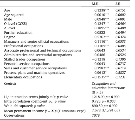
Following Kazarosian (1997), permanent income is proxied by taking the fitted values from modelling the natural loga-rithm of equivalized yearly household income conditioned on gender, a quadratic in age, highest educational attainment, occupational dummy variables and interactions between the education and occupational dummy variables. The results of this specification, which is used to create permanent income, are shown in Table A2 in the appendix. Income volatility is calculated by taking the squared difference of detrended income between the individual’s first and last year in the panel (as an adult) weighted by the number of years in the panel, as is common in the literature (see, for example, Browning and Lusardi,1996; Carroll and Samwick,1998, and Guariglia, 2001).

Summary statistics are provided in Table 1and a correlation matrix of the covariates used in the adult analysis is given in

Table A3in the appendix. The degree of magnitude of the

correla-tion coefficients, even where statistically significant, is relatively small which suggests that co-linearity is unlikely to be problematic in the empirical analysis. Our key covariate of interest is whether the individual saved as a child,SCit. Hence, we focus on the magni-tude, sign and statistical significance ofw1.

3.1.2. Dynamic random effects probit model

The individual may be more likely to save if he/she has saved in the past, which may be particularly important in the context of

regular monthly saving. Hence, in order to explore the robustness of our findings, we explore the effect of allowing for state depen-dence in the individual’s saving behaviour by analysing dynamics over the time period. Thus, we re-estimate Eq. (2) allowing for state dependence by conditioning onSitA1. The likelihood of saving over the period is modelled via a random effects dynamic panel estimator as follows:

SA it ¼1½

p

S

A

it1þG0ithþZ0i

j

þ

a

iþ

x

it>0 ð3aÞ

where the covariates are as defined in Eq.(2)and½X2it;SCit 2Git;Zi. The correlation between the individual effect

_ai

andSA

it1 in the dynamic binary model makesSA

it1endogenous and, hence, the esti-mates will be inconsistent. Wooldridge (2010) suggests an approach to overcome this, where an appropriate treatment of the individual effect can be determined by specifying the following:

a

i¼

a

0þ

a

1SiA0þGi0

g

þ

m

i

m

iNð0;1Þ ð3bÞ

whereSiA0is the initial state, i.e. whether the individual saves when first observed as an adult in the panel. This approach relies on the time invariant characteristics, Zi, and group means of the time varying covariates,Gi, where substitution of Eq.(3b)into(3a) pro-duces an augmented random effects model. The analysis is based on a panel of 4552 observations covering the period 2000–2014. State dependence in terms of the statistical significance of SA

it1 and the size of

_p

, as well as the importance of heterogeneity, as indicated by

q

1¼

r

2a=ð

r

2aþ

r

2xÞ, are investigated by estimating

[image:7.595.43.563.86.389.2]

Eqs. (3a,b). Table 3

Determinants of savings behaviour in early adulthood – ever saved as a child.

Random effects (RE) Random effects (RE) Random effects (RE)

PROBIT Dynamic PROBIT TOBIT

M.E. S.E. M.E. S.E. M.E. S.E.

Saved in previous period – – 0.0690⁄⁄⁄ 0.0165 – –

Age 0.1494⁄⁄⁄ _{0.0256 0.1119}⁄⁄⁄ _{0.0373 0.2950}⁄⁄⁄ _0.0619

Age squared 0.0032⁄⁄⁄ _{0.0006 0.0023}⁄⁄⁄ _{0.0006 0.0062}⁄⁄⁄ _0.0014

Male 0.0041 0.0164 0.2826⁄⁄ 0.1333 0.0088 0.0386

Permanent income 0.0331⁄⁄⁄ 0.0006 0.0460⁄⁄⁄ 0.0084 0.0943⁄⁄⁄ 0.0148

Volatility of income 0.0151⁄ 0.0083 0.0040 0.0061 0.0400⁄ 0.0242

Excellent health 0.0592⁄ 0.0313 0.0140 0.0438 0.1549 0.1122

Good health 0.0776 0.0571 0.0301 0.0396 0.1664 0.1060

Fair health 0.0494 0.0422 0.0263 0.0398 0.0867 0.1084

Number of children 0.0136 0.0092 0.0294⁄ 0.0153 0.0326 0.0228

Married or cohabiting 0.0304 0.0342 0.0279 0.0349 0.0806 0.0822

White 0.0723⁄⁄ 0.0336 0.0279 0.0307 0.1649⁄⁄ 0.0824

Black 0.0752 0.0473 0.0545 0.0401 0.1581 0.1226

Asian 0.0925 0.0675 0.0436 0.0581 0.2878 0.1799

O level (GCSE) 0.0683⁄⁄⁄ _{0.0209 0.0269 0.0309 0.1492}⁄⁄⁄ _0.0519

A level 0.0714⁄⁄⁄ _{0.0217 0.0183 0.0286 0.1995}⁄⁄⁄ _0.0548

Further education 0.0444 0.0322 0.0316 0.0405 0.1474⁄ 0.0796

Degree 0.1289⁄⁄⁄ 0.0324 0.0669⁄ 0.0369 0.3470⁄⁄⁄ 0.0844

Employee 0.1038⁄⁄⁄ 0.0172 0.1275⁄⁄⁄ 0.0228 0.3865⁄⁄⁄ 0.0432

Self employed 0.1019⁄⁄ 0.0501 0.1730⁄⁄⁄ 0.0578 0.5225⁄⁄⁄ 0.1353

Unemployed 0.2264⁄⁄⁄ 0.0303 0.1196⁄⁄⁄ 0.0357 0.5327⁄⁄⁄ 0.0689

Own home outright 0.1295⁄⁄⁄ _{0.0250 0.0376 0.0345 0.3563}⁄⁄⁄ _0.0650

Own home on a mortgage 0.0803⁄⁄⁄ _{0.0194 0.0190 0.0268 0.2297}⁄⁄⁄ _0.0480

Rent home from council 0.0483⁄ 0.0259 0.0240 0.0381 0.1422⁄⁄⁄ 0.0634

Ever saved as a child 0.1450⁄⁄⁄ 0.0182 0.1016⁄⁄⁄ 0.2223 0.3675⁄⁄⁄ 0.0440

Controls Year and region of residence

H0:g¼0;#p value – 46.56p=0.000 –

Intra correlation coefficientq1;p value 0.420p=0.000 0.206p=0.058 0.362p=0.000

Wald chi squared;p value 457.33p=0.000 816.01p=0.000 589.37p=0.000

Observations 7078 4552 7078

3.1.3. Random effects tobit model

Given that the data provides information on the amount of monthly savings, we also estimate a random effects tobit model in order to ascertain whether having saved as a child influences the amount saved on a monthly basis in adulthood:

logðSitAÞ

¼X0

2itk2þw2S

C

itþ

a

iþ

it¼H0itdþ

it ð4Þ

logðSitAÞ ¼max½0;logðS A itÞ

whereSAitis the unobserved untruncated latent dependent variable and SA

it is the censored dependent variable. We report marginal effects on the expected value of logðSA

itÞfor uncensored observa-tions, seeCameron and Trivedi (2005), defined as follows:

@E½logðSA itÞlogðS

A itÞ>0;H

@hk

¼dk 1r H 0_d

r

r2

ð5Þ

wherer¼/H0d

r

=U H0d

r

,/andUdenote the density and cumulative distributions of the standard normal, respectively, hk is the kth covariate from the vector H, and

r

is the standard error of the regression.

In the empirical analysis,SC

itis defined in three ways: firstly, as a binary indicator for whether the individual ever saved as a child; and secondly, by a series of binary indicators for the number of times the individual saved during childhood – once, twice, three times or four or above (never saved is the reference category). Thirdly, whether the individual saved during childhood can be decomposed into whether the child saved to buy things or whether the child saved not to spend, with the reference category of not saving as a child. Saving to buy specific things may capture an apti-tude for budgeting at an early age, whereas saving with no specific purpose may reflect precautionary saving motives. Hence, we also explore if these two different motivations for saving during child-hood have distinct influences on saving behaviour as an adult.

3.1.4. Instrumental variable analysis

A potential criticism of the above empirical approaches is that whether the individual saved as a child might be an endogenous covariate. In order to address this issue, we adopt an instrumental variable approach where we jointly model the probability of saving during childhood and adult saving outcomes (specifically, the probability of saving as an adult and the amount saved as an adult). To do this, we employ a set of instruments which are strongly asso-ciated with the saving decision as a child but are arguably exoge-nous to their saving behaviour as an adult. Hence, we estimate the following joint model in Eqs.(6a) and (6b)as a bivariate probit for analysing the probability of saving as an adult:

SC

i ¼1½X02i

p

1þEXPiP0

p

2þ

m

1i>0 ð6aÞ

SiA¼1½X02i

p

3þ

p

4S

C

i þ

m

2i>0 ð6bÞ

We also model the amount saved as an adult in a joint frame-work where Eqs.(6a) and (6c)are jointly estimated as follows:

logðSiAÞ

¼X0

2i

p

5þ

p

6SCi þ

m

3i logðSiAÞ ¼max½0;logðS

A iÞ

ð6cÞ

We observe the individual during childhood, on average, 3 times, between 1997 to 2001 and 2005, and then as an adult again, on average, 3 times, between 1998 and 2013/14. Although we have panel data, this relates to two distinct time periods, i.e. childhood and adulthood, as shown inFig. 1. By definition, the time periods do not coincide and the length of the two respective panels can also differ. This subsequently means that the IV models given in Eqs. (6a), (6b), (6c) are estimated on cross-sectional data.

Covariates are based on the final time the adult is observed in the panel. In terms of the key variables of interest,SiAis an indica-tor variable for whether the adult saved in the final period observed in the data andSC_i is an indicator variable for whether the individual ever saved during their childhood. Focusing on the final time period that the individual is observed as an adult maximises the gap between saving decisions made as a child, i.e.SCi, and those made when observed in the data for the final time as an adult, i.e.SA

i, where the gap is now 9 years, on average. In terms of modelling the probability of whether the individual saved a child, i.e. Eq.(6a), we include those covariates which are used to model adult saving outcomes, i.e.X2i, and a set of instru-mental variables. The instruments are based on the financial expec-tations of the individual’s parent as given by vectorEXPP

i. These instruments seem plausible from a theoretical point of view in that there is no obvious reason why the financial expectations of the parent, measuredex ante, should influence the current saving beha-viour of their offspring now observed as young adults. One possible mechanism, however, may operate via intergenerational correla-tion in financial attitudes. To attempt to overcome this, we also esti-mate Eq.(6a)jointly with(6d), taking dynamics into account:

SiA¼1½fS A

it1þX02i

p

7þ

p

8S

C

i þ

m

4i>0 ð6dÞ If intergenerational correlation in financial expectations exists, then this should be subsumed into the dynamic effect.18 Based on the results reported in Section2.2, from a statistical viewpoint, parental expectations appear to be valid instruments. The argument here is that there is a direct relationship between the expectations of parents and the saving behaviour of their children, whilst there should be no direct association between parental expectations and the saving behaviour of their offspring when observed as young adults – only an indirect relationship operating through the effect on the probability of saving as a child.

The alternative IV models are all estimated simultaneously by a conditional recursive mixed process estimator (CMP),Roodman

(2011).19 _{The error terms}

m

1i and

m

ji are assumed to be jointly normally distributed, i.e. ð

m

1i;

m

jiÞ0Nð0;RÞ, and the correlation between the equations is given by

q

2¼

r

2m1=ð

r

2m1þ

r

2mjÞ, where j equals 2, 3 or 4.

3.2. Results

3.2.1. Static random effects probit model

The first column ofTable 3summarises the results of estimating

Eq.(2). Clearly, the panel nature of the data is important given the

statistical significance of the

q

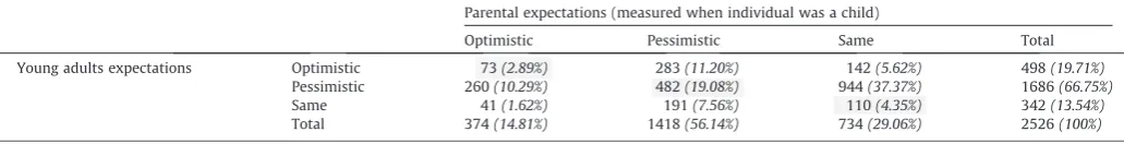
1parameter, indicating that there is

18_{Based on the sample of 2526 young adults, the evidence for the existence of an} intergenerational correlation in financial expectations is weak, given that the correlation between the financial expectations of the individual’s parent and those of the young adult is small in magnitude and statistically insignificant at 0.0237 (p -value = 0.2331).Table A4in the appendix provides a cross tabulation of financial expectations. The low correlation is not surprising given the small proportions observed on the lead diagonal: i.e. young adults, on average, have different financial expectations to that of their parent, where the latter was observed during the individuals’ childhood.

19

[image:9.595.43.565.84.372.2]

Table 4

Determinants of savings behaviour in early adulthood – decomposition.

Random effects (RE) PROBIT Random effects (RE) Dynamic PROBIT

Random effects (RE) TOBIT

M.E. S.E. M.E. S.E. M.E. S.E.

Panel A: Decomposition of ever saving as a child

Saved as a child to buy things 0.1530⁄⁄⁄ _{0.0198 0.1150}⁄⁄⁄ _{0.0214 0.4183}⁄⁄⁄ _0.0510

Saved as a child not to spend 0.1358⁄⁄⁄ _{0.0203 0.0857}⁄⁄⁄ _{0.0220 0.3684}⁄⁄⁄ _0.0527

H0:g¼0;#p value – 46.59p=0.000 –

Intra correlation coefficientq1;p value 0.419p=0.000 0.262p=0.000 0.361p=0.000

Wald chi squared;p value 458.54p=0.000 635.81p=0.000 590.95p = 0.000

Panel B: Number of times saved

Saved as a child 1 time 0.0454⁄⁄⁄ _{0.0135 0.0042}⁄⁄⁄ _{0.0022 0.1338}⁄⁄⁄ _0.0522

Saved as a child 2 times 0.0887⁄⁄⁄ 0.0285 0.0347⁄⁄⁄ 0.0166 0.2750⁄⁄⁄ 0.0741

Saved as child 3 times 0.0895⁄⁄⁄ 0.0257 0.0291⁄⁄⁄ 0.0135 0.2503⁄⁄⁄ 0.0663

Saved as child 4 or more times 0.1455⁄⁄⁄ 0.0259 0.0531⁄⁄⁄ 0.0251 0.3850⁄⁄⁄ 0.0666

H0:g¼0;#p value – 41.88p=0.003 –

Intra correlation coefficientq1;p value 0.434p=0.000 0.285p=0.000 0.376p=0.000

Wald chi squared;p value 426.96p=0.000 608.56p=0.000 558.89p=0.000

Panel C: Decomposition of number of times saved

Saved to buy 1 time 0.1039⁄⁄⁄ 0.0259 0.0927⁄⁄⁄ 0.0264 0.2934⁄⁄⁄ 0.0687

Saved to buy 2 times 0.1667⁄⁄⁄ 0.0287 0.1314⁄⁄⁄ 0.0292 0.5032⁄⁄⁄ 0.0786

Saved to buy 3 times 0.1690⁄⁄⁄ 0.0268 0.1174⁄⁄⁄ 0.0254 0.4697⁄⁄⁄ 0.0730

Saved to buy 4 or more times 0.1741⁄⁄⁄ 0.0308 0.1229⁄⁄⁄ 0.0283 0.5221⁄⁄⁄ 0.0847

Saved to not spend 1 time 0.0434⁄ _{0.0252 0.0257 0.0268 0.1074}⁄⁄⁄ _0.0402

Saved to not spend 2 times 0.0555⁄ _{0.0304 0.0951}⁄⁄⁄ _{0.0328 0.1831}⁄⁄ _0.0803

Saved to not spend 3 times 0.0722⁄⁄⁄ 0.0284 0.0984⁄⁄⁄ 0.0492 0.1931⁄⁄ 0.0742

Saved to not spend 4 or more times 0.1759⁄⁄⁄ 0.0384 0.3023⁄⁄⁄ 0.0987 0.5047⁄⁄⁄ 0.1064

H0:g¼0;#p value – 42.91p=0.002 –

Intra correlation coefficientq1;p value 0.419p=0.000 0.253p=0.000 0.363p=0.000

Wald chi squared;p value 469.11p=0.000 650.15p=0.000 608.21p=0.000

Observations 7078 4552 7078

⁄⁄⁄,⁄⁄,⁄_{Denotes statistical significance at the 1, 5 and 10 percent levels respectively. Controls in each panel are as inTable 3.}#

[image:9.595.43.293.427.730.2]

provides a test of the significance of group means of the time varying covariates in Eq.3(b).

Table 5

Determinants of the amount saved in early adulthood – Heckman model.

M.E./COEF S.E.

Amount saved

Age 0.3878⁄⁄⁄ 0.0964

Age squared 0.0083⁄⁄⁄ 0.0021

Male 0.0629 0.0491

Permanent income 0.0906⁄⁄⁄ 0.0214

Volatility of income 0.0008 0.0267

Excellent health 0.2618 0.1678

Good health 0.0615 0.1618

Fair health 0.0294 0.1728

Number of children 0.0052 0.0325

Married or cohabiting 0.0419 0.1232

White 0.2124⁄ 0.1129

Black 0.3686⁄⁄ _0.1492

Asian 0.2054 0.1994

O level (GCSE) 0.0546 0.0780

A level 0.1154 0.0796

Further education 0.1069 0.1162

Degree 0.1517 0.1149

Employee 0.7145⁄⁄⁄ 0.0624

Self employed 1.0858⁄⁄⁄ _0.1691

Unemployed 0.0020 0.2001

Own home outright 0.1502⁄⁄⁄ 0.0478

Own home on a mortgage 0.2205⁄ 0.1260

Rent home from council 0.1725⁄ 0.0985

Ever saved as a child 0.1358⁄⁄⁄ 0.0433

Probability of saving

Number of problems reported 0.0482⁄⁄ 0.0178

Controls Year and region of residence

Wald chi squared;p value 607.37p=0.000 Intra correlation coefficientq1;p value 0.284p=0.000 Cross equation correlationq2;p value 0.114p=0.000

Observations 7078

⁄⁄⁄,⁄⁄,⁄_{Denotes statistical significance at the 1, 5 and 10 percent levels respectively.}

Coefficients (marginal effects) are reported when modelling the amount saved (probability of saving).

Table 6

Modelling saving as a proportion of real equivalized household income – Ever saved as a child.

M.E. S.E.

Age 0.0234⁄⁄⁄ 0.0066

Age squared 0.0005⁄⁄⁄ 0.0001

Male 0.0019 0.0043

Permanent income 0.0089⁄⁄⁄ 0.0015

Volatility of income 0.0059⁄⁄⁄ _0.0022

Excellent health 0.0239⁄⁄ 0.0117

Good health 0.0229⁄⁄ 0.0111

Fair health 0.0118 0.0115

Number of children 0.0013 0.0024

Married or cohabiting 0.0047 0.0087

White 0.0137 0.0089

Black 0.0130 0.0123

Asian 0.0381⁄⁄ 0.0172

O level (GCSE) 0.0133⁄⁄ 0.0055

A level 0.0172⁄⁄⁄ 0.0057

Further education 0.0118 0.0082

Degree 0.0367⁄⁄⁄ 0.0083

Employee 0.0490⁄⁄⁄ _0.0045

Self employed 0.0586⁄⁄⁄ _0.0127

Unemployed 0.0542⁄⁄⁄ 0.0083

Own home outright 0.0357⁄⁄⁄ 0.0064

Own home on a mortgage 0.0211⁄⁄⁄ 0.0051

Rent home from council 0.0115⁄ 0.0069

Ever saved as a child 0.0374⁄⁄⁄ 0.0048

Controls Year and region of residence

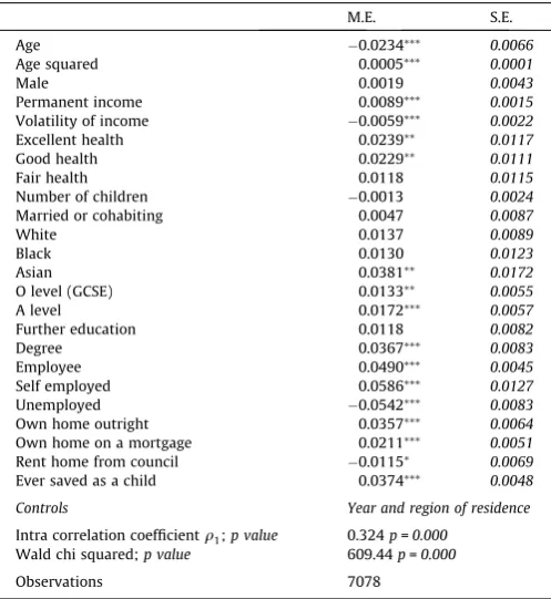
Intra correlation coefficientq1;p value 0.324p=0.000 Wald chi squared;p value 609.44p=0.000

Observations 7078

[image:9.595.313.562.451.722.2]

positive intra-personal correlation in the unobservables over time. Permanent income is positively associated with the probability of saving on a monthly basis, where a 1 percent increase in perma-nent income is associated with approximately a 3.3 percent increase in the likelihood of saving, ceteris paribus. Conversely, income volatility is inversely associated with the likelihood of sav-ing. These findings are consistent with existing evidence in the lit-erature, see, for example,Guariglia (2001). The probability that the individual saves on a monthly basis is increasing in educational attainment, where an individual with a degree is approximately 13 percentage points more likely to save than an individual with

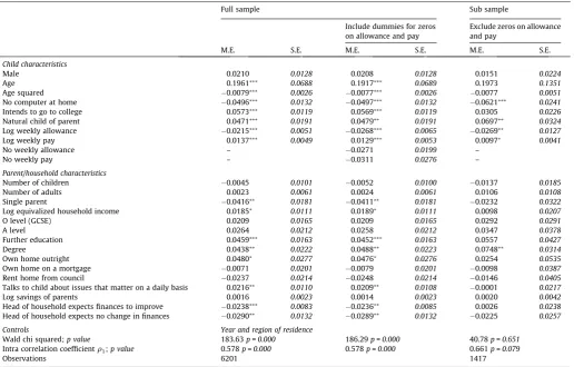
no education. Both the employed and the self-employed are more likely to save on a monthly basis than those not in the labour mar-ket. In contrast, those currently unemployed but seeking work are around 23 percentage points less likely to save. Housing tenure is also important where the results show that individuals who own their home outright or via a mortgage have a higher probability of saving on a monthly basis, which potentially reflects a wealth effect. Whether the individual ever saved during childhood has a large positive association with the probability of saving on a monthly basis in adulthood at 14.5 percentage points and is only outweighed by the effect of unemployment.

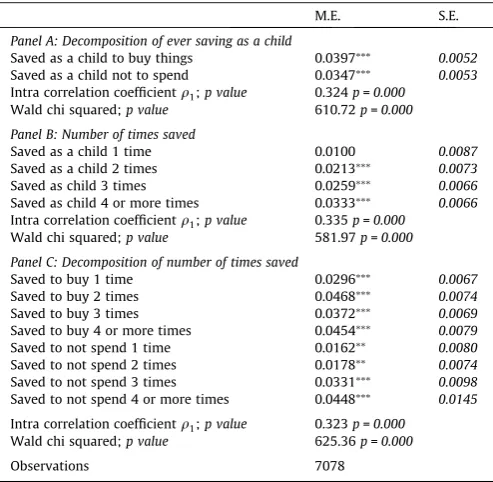
In Panel A of Table 4, we decompose the binary indicator of whether the individual ever saved as a child according to saving motive. Interestingly, whilst saving to buy things and saving not to spend, relative to not having saved during childhood, are both positively associated with the probability of saving as an adult, the dominant effect is from saving to buy things, i.e. 15.3 percent-age points compared to 13.6 percentpercent-age points. It may be the case that individuals who saved as a child specifically to buy things may have acquired important skills in budgeting and setting goals at an early age, which serve to have a particularly large effect on saving behaviour in early adulthood.

In Panel B ofTable 4we define childhood saving,SC

it, as a series of binary variables indicating the number of times that the individ-ual saved during childhood. Clearly, the number of times the indi-vidual saved as a child has an increasing monotonic effect on the probability of saving during adulthood, ranging from 4.5 percent-age points (saved once as a child) through to 14.6 percentpercent-age points (saved four or more times as a child). Such effects are also evident when we decompose the reasons for why the individual saved as a child, see Panel C, where generally saving to buy things dominates. The exception to this is if the child saved four or more times regardless of the motive, where the effect on the probability of currently saving is around 17 percentage points.

3.2.2. Dynamic random effects probit model

[image:10.595.36.283.94.335.2]

To investigate the robustness of the results, we now allow for state dependence, where the results from estimating Eq.(3)are presented in the second column ofTable 3. As with the previous

Table 8

Determinants of savings behaviour in early adulthood – IV analysis.

PROBIT Dynamic PROBIT TOBIT

M.E. S.E. M.E. S.E. M.E. S.E.

First stage summary

Head of household expects finances to improve 0.0458⁄⁄ _{0.0227 0.0436}⁄⁄ _{0.0220 0.0474}⁄ _0.0254 Head of household expects no change in finances 0.0269⁄⁄⁄ 0.0109 0.0291⁄⁄⁄ 0.0111 0.0188⁄⁄⁄ 0.0067 Second stage summary

Saved in previous period – – 0.2337⁄⁄⁄ 0.0274 – –

Ever saved as a child 0.1529⁄⁄⁄ 0.0268 0.1152⁄⁄⁄ 0.0151 0.2375⁄⁄ 0.1046

Controls As inTable 3

H0:p1¼0;1p value 546.79p=0.000 463.82p= 0.000 209.13p=0.000

H0:p2¼0;2p value 17.79p= 0.000 18.06p=0.000 18.44p=0.000

H0:p3¼0;3p value 582.91p=0.000 – –

H0:p5¼0;4p value – – 169.18p=0.000

H0:g;p1¼0;5p value – 318.28p=0.000 –

Cross equation correlationq2;p value 0.767p=0.000 0.828p=0.000 0.182p=0.000

Sargan-Hausman test 2.36p=0.3073 1.81p= 0.4055 0.01p=0.9950

Wald chi squared;p value 554.64p=0.000 840.47p=0.000 662.95p=0.000

Observations 2526 2526 2526

⁄⁄⁄,⁄⁄,⁄_{Denotes statistical significance at the 1, 5 and 10 percent levels, respectively.}1

provides a joint test of the significance of covariates (excluding the instruments) in the first stage, Eq.(6a);2_{provides a joint test of the significance of the instruments, i.e. expectations, used in the first stage, Eq.(6a);}3_{provides a joint test of the significance of} covariates (excluding whether the individual saved during childhood) used in the second stage when modelling the probability that the adult saves, Eq.(6b);4

provides a joint test of the significance of covariates (excluding whether the individual saved during childhood) used in the second stage when modelling the amount that the adult saves, Eq. (6c); and5

[image:10.595.33.555.524.702.2]

provides a joint test of the significance of covariates (excluding whether the individual saved during childhood) including group means of the time varying covariates used in the second stage when modelling the probability that the adult saves allowing for dynamics, Eq.(6d).

Table 7

Modelling saving as a proportion of real equivalized household income – Decomposition.

M.E. S.E.

Panel A: Decomposition of ever saving as a child

Saved as a child to buy things 0.0397⁄⁄⁄ _0.0052 Saved as a child not to spend 0.0347⁄⁄⁄ 0.0053 Intra correlation coefficientq1;p value 0.324p=0.000

Wald chi squared;p value 610.72p=0.000

Panel B: Number of times saved

Saved as a child 1 time 0.0100 0.0087

Saved as a child 2 times 0.0213⁄⁄⁄ _0.0073

Saved as child 3 times 0.0259⁄⁄⁄ 0.0066

Saved as child 4 or more times 0.0333⁄⁄⁄ 0.0066 Intra correlation coefficientq1;p value 0.335p=0.000

Wald chi squared;p value 581.97p=0.000

Panel C: Decomposition of number of times saved

Saved to buy 1 time 0.0296⁄⁄⁄ _0.0067

Saved to buy 2 times 0.0468⁄⁄⁄ 0.0074

Saved to buy 3 times 0.0372⁄⁄⁄ 0.0069

Saved to buy 4 or more times 0.0454⁄⁄⁄ 0.0079

Saved to not spend 1 time 0.0162⁄⁄ 0.0080

Saved to not spend 2 times 0.0178⁄⁄ 0.0074

Saved to not spend 3 times 0.0331⁄⁄⁄ _0.0098

Saved to not spend 4 or more times 0.0448⁄⁄⁄ _0.0145

Intra correlation coefficientq1;p value 0.323p=0.000 Wald chi squared;p value 625.36p=0.000

Observations 7078

⁄⁄⁄,⁄⁄_{Denotes statistical significance at the 1 and 5 percent levels respectively.}

results, there is evidence of unobserved heterogeneity in explain-ing unsystematic variation in the errors. State dependence is clearly important since the coefficient associated with the lagged dependent variable is statistically significant and large in terms of magnitude. Specifically, whether the individual saved in the pre-vious period is associated with around a 7 percentage point higher probability of currently saving. Whilst some covariates have now been driven to statistical insignificance, the influence of whether the individual ever saved as a child remains in terms of both statis-tical significance and magnitude. Indeed, the influence of whether the individual saved as a child is of similar magnitude to that reported in the previous results where the lagged dependent vari-able was not included. The second column of Table 4 Panel A decomposes whether the individual saved as a child into the rea-sons for saving. As found above, the dominant effect stems from saving to buy things, which increases the likelihood of saving as an adult by around 12 percentage points. Focusing on the number of times the individual saved as a child, the effects are similar to those found previously in that the probability of currently saving increases monotonically with the number of times saved as a child, see Panels B and C.

3.2.3. Random effects tobit model

The final column ofTable 3presents the results from estimating Eq.(4)with marginal effects reported based on Eq.(5). Given that the dependent variable is logged and whether the individual saved as a child is a binary variable, the marginal effect can be inter-preted asw2100%. Hence, whether the individual ever saved as a child is associated with a 36 percentage point higher level of monthly savings, conditional on the individual saving in adult-hood. This estimate is clearly large and only outweighed by the effects of labour market status. In order to investigate the magni-tude stemming from childhood saving, we employ an alternative estimator as a robustness check.

It is plausible that the large effect discussed above could be dri-ven by the inclusion in the estimation of Eq.(4) of those adults with zero savings.20_{Hence, in order to investigate this further, we}

employ a Heckman model where the probability of saving as a young adult is jointly modelled alongside the amount saved (for savers). This requires the availability of an instrumental variable which influ-ences the decision to save but has no effect on the amount saved. The instrument we employ is based on the number of financial problems reported in the household. Both the BHPS and UKHLS contain a range of detailed questions relating to household finances of which a sub-set are consistent between the two surveys. Firstly, information is available relating to whether households have difficulty paying for accommodation. Secondly, information on financial hardship at the household level can be discerned from the responses of the head of household regarding the ability of the household to afford to: keep their home adequately warm; be able to pay for a week’s annual hol-iday; replace worn-out furniture; and be able to buy new, rather than second-hand, clothes or buy things for themselves. We create a count of the number of problems reported,CNPit, and use this to explain the probability the adult saves. The Heckman model takes the following form:

SA

it¼1½

u

CNPitþ

a

iþ

s

1it>0 ð7aÞ

logðSitAÞ ¼X02ith1þh2SCitþ

a

iþ

s

2it ð7bÞ

where Eq.(7a)represents the selection equation, i.e. whether the individual saves, and Eq.(7b)represents the amount saved which is a continuous variable. The model incorporates random effects,

and, hence, allows for both intra-personal correlation in saving behaviour over time,

q

1, and cross equation correlation, defined as

_q

₂.21

The results of the analysis are shown inTable 5, where our key parameters of interest are

u

andh2. Clearly, there is evidence of intra-correlation in the observables over time, since

q

1–0, and cor-relation between the probability of saving and the amount saved since

_q

₂–0. A one standard deviation increase in the number of problems reported by the individual decreases the likelihood of saving by just under 5 percentage points (given a standard devia-tion in the number of problems of 0.96).22In terms of the amount saved per month, there is still a positive and statistically significant association with having saved as a child. However, not surprisingly, as compared to the tobit analysis, the magnitude of the effect is somewhat smaller, where having saved during childhood is associ-ated with around saving approximately 14 percentage points more per month as an adult. Hence, in the remaining tobit analysis which follows, the magnitude stemming from having saved as a child should be considered with this in mind.

Returning to the tobit estimates, when decomposing the reason for why the individual saved as a child, as found above, the domi-nant effect stems from saving to buy things, seeTable 4Panel A. In the alternative specifications, where we control for the number of times the individual saved during childhood, it is apparent that an individual who saved four or more times as a child would have nearly one and a half times the level of monthly savings as an indi-vidual who did not save as a child, see Panel B. As found when focusing on the probability of saving, the level of savings is increas-ing monotonically in the number of times saved as a child and this is also apparent once we decompose savings during childhood into the two motives, see Panel C.23

As an alternative to modelling the amount that the adult saves, i.e. the log level, we also analyse monthly savings as a proportion of equivalized monthly household income. This is estimated as a ran-dom effects tobit model with the results shown inTable 6, where it can be seen that whether the individual saved during their child-hood is associated with 3.7 percentage points higher savings as a proportion of income as an adult. The results are consistent with those found for the level of savings in that saving during childhood to buy things has the dominant influence on savings as a propor-tion of household income as an adult, seeTable 7Panels A and C, and the proportion saved is increasing monotonically in the num-ber of times the individual saved as a child, see Panels B and C.

3.2.4. Instrumental variable analysis

To assess the robustness of the findings and, in addition, to explore whether saving during childhood can be treated as an exogenous variable,Table 8provides a summary of the findings from the instrumental variable analysis, where we endogenise sav-ing as a child by jointly estimatsav-ing: a bivariate probit model, Eqs. (6a) and (6b); a static probit model and a dynamic probit model,

Eqs. (6a) and (6d); and a probit and tobit model, Eqs. (6a) and

(6c). The first part ofTable 8reports the first stage results:

specif-ically, the marginal effects associated with the financial expecta-tions of the parent,

p

2. The analysis from the first stage is consistent with that reported in Table 2, which examined the determinants of the child’s saving behaviour. In particular, com-pared to having a parent who was financially pessimistic (as

20

We are very grateful to an anonymous reviewer for highlighting this point.

21

We use the ‘cmp’ routine in STATA to estimate the Heckman model.

22 _{If we include the number of problems reported in the amount saved per month it} is statistically insignificant, thereby supporting its use as an instrument.

23