Representing the Australian Heat Low in a GCM Using Different Surface and Cloud Schemes

(1)

Research Article

Representing the Australian Heat Low in a GCM Using

Different Surface and Cloud Schemes

Matthew M. Allcock and Duncan Ackerley

ARC Centre of Excellence for Climate System Science, School of Earth, Atmosphere and Environment, Monash University, Clayton, VIC 3800, Australia

Correspondence should be addressed to Duncan Ackerley; [email protected]

Received 9 April 2015; Accepted 16 September 2015

Academic Editor: Hiroyuki Hashiguchi

Copyright © 2016 M. M. Allcock and D. Ackerley. This is an open access article distributed under the Creative Commons Attribution License, which permits unrestricted use, distribution, and reproduction in any medium, provided the original work is properly cited.

The high insolation during the Southern Hemisphere summer leads to the development of a heat low over north-west Australia, which is a significant feature of the monsoon circulation. It is therefore important that General Circulation Models (GCMs) are able to represent this feature well in order to adequately represent the Australian Monsoon. Given that there are many different configurations of GCMs used globally (such as those used as part of the Coupled Model Intercomparison Project), it is difficult to assess the underlying causes of the differences in circulation between such GCMs. In order to address this problem, the work presented here makes use of three different configurations of the Australian Community Climate and Earth System Simulator (ACCESS). The configurations incorporate changes to the surface parameterization, cloud parameterization, and both together (surface and cloud) while keeping all other parameterized processes unchanged. The work finds that the surface scheme has a larger impact on the heat low than the cloud scheme, which is caused by differences in the soil thermal inertia. This study also finds that the differences in the circulation caused by changing the cloud and surface schemes together are the linear sum of the individual perturbations (i.e., no nonlinear interaction).

1. Introduction

The high insolation and surface heating of the Australian land surface in summer (December, January, and February (DJF)) create a strong diurnal cycle in temperature and circulation [1–4]. During the daytime, solar heating of the land surface acts to warm the air in the low-level atmosphere, which then rises, lowering the surface pressure. This area of low pressure is known as a heat low. Conversely, as the surface cools at night, a stable nocturnal boundary layer forms, allowing the development of a low-level jet and convergence over the heat low [5]. The boundary layer becomes unstable in the morning (following surface heating), which initiates convection and a reduction in surface pressure as described above. Heat lows also occur in other semiarid areas of the world, for example, the Iberian Peninsula [6–9] and West Africa [10–13].

The heat low circulation is an important feature of the Australian monsoon [14], which resides in the north-west of the continent (see Figure 1(a), the circulation is centred

at approximately 120∘E and 22∘S). It is therefore important to represent the heat low accurately in general circulation models (GCMs) in order to correctly simulate the Australian monsoon system. Previous work by Ackerley et al. [15] shows that the diurnal change in the low-level circulation across the north-west Australian heat low is represented well in the Australian Community Climate and Earth System Simulator version 1.3 (ACCESS1.3). Moreover, Ackerley et al. [16] also show that other GCMs (available as part of the Coupled Model Intercomparison Project phase 5 (CMIP5) including ACCESS1.3 and ACCESS1.0) are also capable of simulating the correct diurnal variation in the low-level circulation. Nevertheless, the magnitudes of the simulated mean wind velocities around the heat low are different for each model by approximately 2–4 m s−1(approximately 50%; see Figure6in [16]). Given the different configurations of the CMIP5 mod-els, Ackerley et al. [16] do not attribute the differences in the heat low circulation to any specific parameterization scheme. Experiments in which changes are applied individually and

(2)

4

110∘E ₁₂₀∘E ₁₃₀∘E ₁₄₀∘E 10∘_S

20∘S

30∘S

(a)

2

110∘E ₁₂₀∘E ₁₃₀∘E ₁₄₀∘E 10∘S

20∘S

30∘_S

(b)

2

110∘_E ₁₂₀∘_E ₁₃₀∘_E ₁₄₀∘_E

10∘_S

20∘_S

30∘S

(c)

2

110∘_E ₁₂₀∘_E ₁₃₀∘_E ₁₄₀∘_E

10∘_S

20∘S

30∘S

(d)

2

110∘E ₁₂₀∘E ₁₃₀∘E ₁₄₀∘E 10∘_S

20∘_S

30∘S

(e)

2

110∘_E ₁₂₀∘_E ₁₃₀∘_E ₁₄₀∘_E

10∘S

20∘_S

30∘_S

(f)

(3)

in combination with the model physics would therefore be useful in order to help identify the important processes that cause the GCMs assessed by Ackerley et al. [16] to differ.

This study builds on the work by Ackerley et al. [15, 16] by evaluating the simulated north-west Australian heat low in three versions of ACCESS with different parameterizations (see Section 2). Therefore, by comparing each of the simula-tions against each other, this paper shows which of the physics changes has the largest impact on the north-west Australian heat low.

The aims of this paper are twofold:

(1) To identify and discuss the differences in the simulated summertime circulation over north-west Australia between three different configurations of ACCESS. (2) To identify the physical processes within each of the

model configurations that causes the differences in the circulation.

A description of the model configurations used in this study is given in Section 2 along with the experimental design and boundary conditions. The main results for the differences in the flow and temperature fields are given in Section 3 and a discussion of why those differences occur is given in Section 4. The main conclusions and suggested further work are given in Section 5.

2. Methods

The Australian Community Climate and Earth System Sim-ulator (ACCESS) is a series of coupled climate models developed in a partnership between the Commonwealth Scientific and Industrial Research Organisation (CSIRO) and the Bureau of Meteorology [17, 18]. This model (ACCESS) is used extensively in climate research and is Australia’s most comprehensive climate model.

The three configurations of ACCESS used in this study are ACCESS1.0 (from now A1.0), ACCESS1.1 (A1.1), and ACCESS1.3 (A1.3). A1.0 is considered as the base version of the model in this study. It utilises the Met Office Surface Exchange Scheme version 2 (MOSES2) land surface model [19] and atmospheric physics from the Hadley Centre Global Environment Model 2 (HadGEM2(r1.1), [20, 21]). A1.1 has the same atmospheric module as A1.0 but uses the Community Atmosphere Biosphere Land Exchange model version 1.8 (CABLE1.8, [19, 22, 23]) instead of MOSES. The main differ-ences between MOSES and CABLE1.8 (which are described in more detail in [23]) applicable to this study are as follows:

(i) MOSES has four vertical levels (at 0.1 m, 0.25 m, 0.65 m, and 2.0 m depth) whereas CABLE1.8 has six vertical levels (at 0.022 m, 0.058 m, 0.154 m, 0.409 m, 1.085 m, and 2.872 m depth).

(ii) MOSES represents nine surface types (five vegetated and four nonvegetated) with each grid box split into nine tiles that can be set to any combination of the nine surface types.

(iii) CABLE1.8 represents thirteen surface types (of which 10 are vegetated) with each grid box split into five

tiles that can be set to any combination of the thirteen surface types.

A1.3 also uses the CABLE1.8 surface scheme but differs from ACCESS1.1 in the representation of clouds. The main differences between the A1.1 (and A1.0) and the A1.3 cloud schemes are as follows:

(i) Cloud inhomogeneities are represented in A1.3 using the “Tripleclouds” scheme [24, 25] but are not repre-sented in A1.0 or A1.1.

(ii) A1.0 and A1.1 use a diagnostic cloud scheme for both liquid and ice cloud fractions [26, 27].

(iii) A1.3 uses the Prognostic Cloud Prognostic Conden-sate scheme (PC2, [28–30]), which treats cloud liquid water and ice content, liquid and ice cloud fraction, and total cloud fraction as prognostic variables.

The different configurations of ACCESS will allow us to identify the impact of

(1) changing the land surface scheme (A1.1 relative to A1.0),

(2) changing the cloud scheme (A1.3 relative to A1.1),

(3) changing both the land surface and cloud schemes (A1.3 relative to A1.0),

on the summertime circulation over north-west Australia. Given that the CMIP5 models assessed in Ackerley et al. [16] use many different combinations of parameterizations, this study presents an opportunity to identify whether the surface scheme, cloud scheme, or both together play the dominant role in governing the Australian heat low structure.

(4)

10m/s

280 286 292 298 304 310

Potential temperature (K)

110∘E 120∘E 130∘E 140∘E

10∘_S

20∘_S

30∘_S

(a)

10m/s

280 286 292 298 304 310

110∘_E ₁₂₀∘_E ₁₃₀∘_E ₁₄₀∘_E

10∘_S

20∘_S

30∘_S

(b)

10m/s

280 286 292 298 304 310

110∘E 120∘E 130∘E 140∘E

10∘S

20∘_S

30∘_S

(c)

10m/s

280 286 292 298 304 310

110∘E ₁₂₀∘E ₁₃₀∘E ₁₄₀∘E

10∘S

20∘S

30∘S

[image:4.600.68.530.72.539.2]

(d)

model configuration are also comparable with the differences relative to the observations (Figures 1(e) and 1(f)). Therefore, this study will focus only on the differences between the model configurations and not the models and observations, which have already been shown in more detail by Ackerley et al. [15, 16], Bi et al. [19], and Kowalczyk et al. [22, 23].

3. Results

3.1. Diurnal Cycle in A1.0. The main climatological features of the A1.0 simulation are described in this section in order to provide a benchmark from which to look at the changes in circulation that are caused by the different model

physics. The mean diurnal cycle of the temperature and horizontal wind at 925 hPa is illustrated in Figure 2 for A1.0. The largest temperature change at 925 hPa (approximately 6 K) occurs between 120–130∘E and 20–25∘S between 0800 and 1400 AWST (Figures 2(a) and 2(b)). There is also a cyclonic circulation centred on 125∘E and 20∘S at 0800 AWST (Figure 2(a)), which weakens and turns towards the centre of the heat low as the low-level air heats up (Figure 2(b)). The change in circulation between 0800 and 1400 AWST is caused by increased low level drag from the presence of dry convection (as discussed in [15, 16]).

(5)

50000 55000 60000 65000 70000 75000 80000 85000 90000 95000

Air p

ressur

e (P

a)

−35

−1 −3

−5

−3 −1

−7

−30 −25 −20 −15 −10

Latitude (degrees)

290 294 298 302 306 310 314 318 322 326 2m/s

9 11

5

3 1

1 ₃

5

(a)

50000 55000 60000 65000 70000 75000 80000 85000 90000 95000

Air p

ressur

e (P

a)

290 294 298 302 306 310 314 318 322 326 −35

−3

−5

−1

−7

−3 −1

−30 −25 −20 −15 −10

Latitude (degrees)

2m/s

13 11

9 7

5 1

1 3

5 3

(b)

50000 55000 60000 65000 70000 75000 80000 85000 90000 95000

Air p

ressur

e (P

a)

−35 −30

−1

−7 −5 ₋₃

−3 −1

−5 −7

−25 −20 −15 −10

Latitude (degrees)

290 294 298 302 306 310 314 318 322 326 2m/s

13

11 9 5

7

3 1 ₁

3

5

(c)

50000 55000 60000 65000 70000 75000 80000 85000 90000 95000

Air p

ressur

e (P

a)

290 294 298 302 306 310 314 318 322 326

−35 −30 −25 −20 −15 −10

Latitude (degrees)

2m/s

13

11 9

5

1 3

3 3

1

1 −1

−1−9

−7

−5 −3

−5

−1−3

(d)

Figure 3: Climatological mean (1979–2001) potential temperature (K), horizontal and vertical wind (m s−1) along 125∘E in A1.0 at (a) 0800 AWST, (b) 1400 AWST, (c) 2000 AWST, and (d) 0200 AWST. The colors indicate potential temperature and the black contours indicate the zonal winds, respectively. The dotted and solid black lines represent zonal flow into and out of the page, respectively. The vertical component is multiplied by a factor of 100 to make it visible.

(Figures 2(c) and 2(d)) as a result of radiative cooling after sunset. This cooling causes the nocturnal boundary layer to form, which reduces the low-level drag. The circulation responds by initially accelerating towards the centre of the heat low at 2000 AWST relative to 1400 AWST (cf. Figures 2(b) and 2(c)) before turning anticyclonically (i.e., away from the heat low centre) between 2000 AWST and 0200 AWST (cf. Figures 2(c) and 2(d)) as the flow tends towards geostrophic balance. The circulation is consistent with the results for A1.0 shown in Ackerley et al. [16].

In order to evaluate the vertical structure of the heat low, a vertical cross section of potential temperature and the wind field along 125∘E is plotted in Figure 3. The surface heating and the subsequent convective mixing (just above the surface) disrupt the stable nocturnal boundary layer between 0800 and 1400 AWST and cause the isentropes to intersect

with the surface (Figures 3(a) and 3(b)). This warm, low-level air rises parallel to the isentropes, causing cool inflow from the north and south (Figure 3(b)). The strongest radial flow into the heat low centre (approximately 4 ms−1) occurs around 2000 AWST (Figure 3(c)), which causes the strongest vertical velocities to occur. This low-level convergence at 2000 AWST is accompanied by increased cyclonic circulation between 950 and 900 hPa and a strengthening of the southerly and easterly flow at approximately 700 to 600 hPa (Figures 2(c) and 3(c)). The structure of the simulated temperature and circulation features in A1.0 are consistent with the features presented by Spengler and Smith [34] for heat low circulations over flat terrain.

(6)

features are very similar to those plotted for A1.0. Instead, the differences in the circulation between A1.1 and A1.0 are now considered to identify the impact of using the CABLE1.8 surface scheme instead of MOSES.

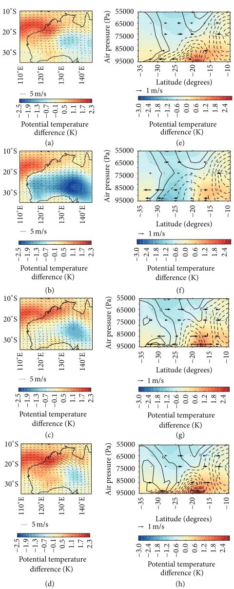
The differences in the mean diurnal cycle of the horizontal winds and air temperature at 925 hPa are plotted in Figures 4(a)–4(d). At 0800 AWST (Figure 4(a)), A1.1 is warmer than A1.0 by approximately 0.1–1.0 K westward of 130∘E with stronger easterly flow over much of the land surface. By 1400 AWST (Figure 4(b)), however, A1.1 is cooler than A1.0 by approximately 1.0 K over much of Australia. The easterly anomalies remain present but weaken (by approximately 3-4 m s−1) between 0800 and 1400 AWST (cf. Figures 4(a) and 4(b)). At 2000 AWST (Figure 4(c)), the differences in 925 hPa temperature are almost zero westward of 130∘E and southward of 20∘S; however, northward of 20∘S, A1.1 is approximately 1 K warmer than A1.0. A1.1 then becomes warmer than A1.0 by 0.5 to 1.5 K westward of 130∘E by 0200 AWST (Figure 4(d)). The easterly anomalies in A1.1 relative to A1.0 are at their strongest (approximately 5 m s−1) at 2000 and 0200 AWST northward of 20∘S and appear to be more divergent over the heat low.

The vertical cross sections of potential temperature and the tangential, radial, and vertical winds in A1.1 relative to A1.0 are plotted in Figures 4(e)–4(h). The warmer temperatures northward of 20∘S at 925 hPa extend verti-cally to approximately 750 hPa at all times (Figures 4(e)– 4(h)), although the anomalies are weakest at 1400 AWST (Figure 4(f)) and strongest at 0200 AWST (Figure 4(h)). The cold anomaly southward of 20∘S at 925 hPa extends from the surface to 650 hPa at 1400 AWST where it connects with another cold anomaly above (Figure 4(f)). The radial wind anomalies are directed away from the centre of the heat low (at approximately 22.5∘S), which is indicative of reduced convergence during the day and night in A1.1 relative to A1.0 (see Figures 4(e)–4(h)).

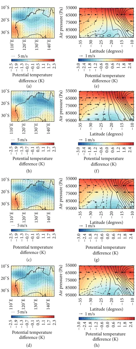
3.3. A1.3 Relative to A1.1. The differences in circulation between A1.3 and A1.1 are considered in this section to identify the impact of changes to the cloud scheme on the heat low. The 925 hPa temperatures are typically 0.5–1.5 K cooler in A1.3 relative to A1.1 with the largest negative anomalies at 1400 and 2000 AWST (Figures 5(b) and 5(c)) and the smallest negative anomalies at 0800 AWST (Figure 5(a)). The differences in the 925 hPa flow are typically 1-2 m s−1 with weak easterly anomalies at the western coast of Australia and northerly (southerly) anomalies at 0800–1400 AWST (2000– 0200 AWST) around 140∘E.

A vertical cross section of the temperature and circu-lation fields along 125∘E is plotted in Figures 5(e)–5(h) for A1.3 relative to A1.0. The cold anomalies at 925 hPa extend from the surface to approximately 800 hPa and vary little throughout the day (except below 900 hPa). Moreover, the air temperatures are 1-2 K warmer in A1.3 relative to A1.1 above the cold anomaly. Again, there is little diurnal change to the temperatures above 750 hPa. Similarly, there is little change in the tangential wind field at 125∘E (approximately within

±1 m s−1); however, the radial wind strengthens towards

the centre of the heat low at all levels between 0800 and 1400 AWST (Figures 5(e) and 5(f)) before weakening towards 0200 AWST (Figures 5(g) and 5(h)). The strengthening of the radial wind onshore suggests that there is stronger conver-gence over the land during the day in A1.3 relative to A1.1.

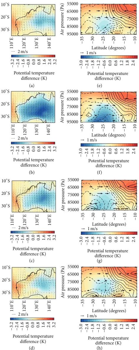
3.4. A1.3 Relative to A1.0. As with A1.1, A1.3 is cooler (by approximately 1.5 K) at 925 hPa over much of Australia at 1400 AWST (Figure 6(b)) before warming by approximately 0.1–0.5 K over the north-west of the continent overnight (Figure 6(d)). The A1.3 simulation is also more easterly at 925 hPa over the majority of the Australian land mass throughout the day with the strongest flow anomalies located near 20∘S (approximately 3 m s−1).

The negative temperature anomalies in A1.3 relative to A1.0 extend from the surface to 700 hPa and are largest in magnitude at 1400 AWST (Figure 6(f)). The low-level (below 900 hPa) warm anomaly in A1.3 relative to A1.0 develops and strengthens to approximately +0.6 K by 0200 AWST (cf. Figures 6(f)–6(h)) and persists to 0800 AWST (Figure 6(a)). Above 700 hPa the potential temperature is typically 1-2 K higher in A1.3 relative to A1.0. The stronger 925 hPa easterly flow in A1.3 relative to A1.0 at 0200 AWST (Figure 6(d)) is restricted to below 750 hPa. Moreover, the differences in the radial flow in A1.3 relative to A1.0 indicate that there is weaker nocturnal convergence over the land at 2000 AWST (Figure 6(g)) in A1.3.

4. Discussion

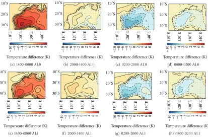
4.1. A1.1 Relative to A1.0. The main difference in the diurnal cycle between A1.1 and A1.0 is that the low-level atmosphere (below approximately 800 hPa) over the heat low is cooler during the day and warmer overnight in A1.1 compared with A1.0 (see Figure 4). To illustrate this, the differences in 925 hPa temperatures across consecutive 6-hour periods are plotted in Figure 7. From 0800 to 1400 AWST A1.1 warms by 4.0–7.0 K over most of Australia whereas the 925 hPa temperatures increase by 5.0–8.0 K in A1.0 (and is conse-quently hotter) by 1400 AWST. Between 1400 to 2000 AWST, A1.1 and A1.0 both warm by similar amounts (approximately 1.0–2.0 K, Figures 7(b) and 7(f)); however, between 2000 and 0200 AWST A1.0 cools down faster than A1.1 and is consequently cooler overnight. The diurnal range in the 925 hPa temperatures is therefore smaller in A1.1 than A1.0.

(7)

110

∘ E

120

∘E

13

0

∘E

14

0

∘ E 10∘S

20∘S 30∘_S

−2.5 −1.9 −1.3 −0.7 −0.1 0.5 1.1 1.7 2.3

Potential temperature difference (K)

110

∘E

120

∘E

13

0

∘E

14

0

∘E 10∘S

20∘S

30∘S

−2.5 −1.9 −1.3 −0.7 −0.1 0.5 1.1 1.7 2.3

110

∘ E

120

∘E

13

0

∘E

14

0

∘E 10∘_S

20∘_S

30∘_S

−2.5 −1.9 −1.3 −0.7 −0.1 0.5 1.1 1.7 2.3

110

∘ E

120

∘E

13

0

∘E

14

0

∘E 10∘S

20∘_S

30∘S

−2.5 −1.9 −1.3 −0.7 −0.1 0.5 1.1 1.7 2.3

−2.4 −1.8 −1.2 −0.6 0.0 0.6 1.2 1.8 2.4

−3.0

− 2

− 2 − 3 − 1

− 3 _{− 1} 0

0

Potential temperature difference (K) 95000

85000 75000 65000 55000

Air p

ressur

e (P

a)

−1

5

−3

0

−2

0

−2

5

−1

0

−3

5

Latitude (degrees)

(e) (a)

(b)

(c)

(d)

− 1

− 1− 2 − 3

−2.4 −1.8 −1.2 −0.6 0.0 0.6 1.2 1.8 2.4

−3.0

0

1

85000 75000 65000 55000

Air p

ressur

e (P

a)

−1

0

−2

5

−2

0

−1

5

−3

0

−3

5

Latitude (degrees)

(f)

− 1 − 1 1

0 0

− 2 − 3

−2.4 −1.8 −1.2 −0.6 0.0 0.6 1.2 1.8 2.4

−3.0

1

85000 75000 65000 55000

Air p

ressur

e (P

a)

−3

0

−2

0

−1

5

−1

0

−2

5

−3

5

Latitude (degrees)

(g)

− 1 − 3 − 2 − 1 − 3 − 4 − 2 1

0 0

−2.4 −1.8 −1.2 −0.6 0.0 0.6 1.2 1.8 2.4

−3.0

−3

5

−3

0

−2

5

−2

0

−1

5

−1

0

Latitude (degrees)

85000 75000 65000 55000

Air p

ressur

e (P

a)

(h) 5m/s

5m/s

1m/s

[image:7.600.179.419.66.670.2]

(8)

110

∘ E

120

∘ E

13

0

∘ E

14

0

∘ E 10∘_S

20∘_S

30∘S

−2.5 −1.9 −1.3 −0.7 −0.1 0.5 1.1 1.7 2.3

110

∘E

120

∘E

13

0

∘E

14

0

∘E 10∘S

20∘_S

30∘S

−2.5 −1.9 −1.3 −0.7 −0.1 0.5 1.1 1.7 2.3

110

∘ E

120

∘ E

13

0

∘ E

14

0

∘ E 10∘_S

20∘S 30∘_S

−2.5 −1.9 −1.3 −0.7 −0.1 0.5 1.1 1.7 2.3

110

∘ E

120

∘E

13

0

∘E

14

0

∘E 10∘S

20∘S 30∘_S

−2.5 −1.9 −1.3 −0.7 −0.1 0.5 1.1 1.7 2.3

−2.4 −1.8 −1.2 −0.6 0.0 0.6 1.2 1.8 2.4

−3.0

− 2

− 1 3 2 1 0

0 0

85000 75000 65000 55000

Air p

ressur

e (P

a)

−3

5

−2

5

−2

0

−1

0

−1

5

−3

0

Latitude (degrees)

− 1 3

1 2 4 − 2

−2.4 −1.8 −1.2 −0.6 0.0 0.6 1.2 1.8 2.4

−3.0

0

85000 75000 65000 55000

Air p

ressur

e (P

a)

−3

0

−3

5

−2

0

−1

0

−2

5

−1

5

Latitude (degrees)

− 2

− 1 1 2 3 0

0 4

−2.4 −1.8 −1.2 −0.6 0.0 0.6 1.2 1.8 2.4

−3.0

Air p

ressur

e (P

a) 55000 65000

75000

85000

95000

−2

0

−3

5

−3

0

−1

5

−1

0

−2

5

Latitude (degrees)

− 2 − 1

1 ₃ 4 0

2 0

0

−2.4 −1.8 −1.2 −0.6 0.0 0.6 1.2 1.8 2.4

−3.0

85000 75000 65000 55000

Air p

ressur

e (P

a)

−1

0

−3

5

−1

5

−3

0

−2

5

−2

0

Latitude (degrees)

(a) (e)

(b) (f)

(c) (g)

(d) (h)

5m/s

1m/s

[image:8.600.182.417.65.667.2]

(9)

110

∘ E

120

∘ E

13

0

∘ E

14

0

∘ E 10∘_S

20∘S

30∘S

−3.2 −2.4 −1.6 −0.8 0.0 0.8 1.6 2.4 3.2

110

∘ E

120

∘ E

13

0

∘ E

14

0

∘ E 10∘_S

20∘S

30∘S

−3.2 −2.4 −1.6 −0.8 0.0 0.8 1.6 2.4 3.2

110

∘ E

120

∘E

13

0

∘E

14

0

∘ E 10∘S

20∘S 30∘_S

−3.2 −2.4 −1.6 −0.8 0.0 0.8 1.6 2.4 3.2

110

∘E

120

∘E

13

0

∘ E

14

0

∘ E 10∘_S

20∘S

30∘S

−3.2 −2.4 −1.6 −0.8 0.0 0.8 1.6 2.4 3.2

−2.4 −1.8 −1.2 −0.6 0.0 0.6 1.2 1.8 2.4

−3.0

− 3− 2 − 1 − 1

12 3

0

85000 75000 65000 55000

Air p

ressur

e (P

a)

−2

0

−1

5

−3

0

−1

0

−3

5

−2

5

Latitude (degrees)

−2.4 −1.8 −1.2 −0.6 0.0 0.6 1.2 1.8 2.4

−3.0

− 1 − 1 0

0 0 1 2 3 4

85000 75000 65000 55000

Air p

ressur

e (P

a)

−2

5

−3

5

−2

0

−1

0

−3

0

−1

5

Latitude (degrees)

−2.4 −1.8 −1.2 −0.6 0.0 0.6 1.2 1.8 2.4

−3.0

− 1 − 2 − 1

0

1 3 3 2

85000 75000 65000 55000

Air p

ressur

e (P

a)

−3

0

−2

5

−2

0

−1

5

−1

0

−3

5

Latitude (degrees)

− 1 − 2 1

1 2 3

0 1

0

− 3 − 4

−2.4 −1.8 −1.2 −0.6 0.0 0.6 1.2 1.8 2.4

−3.0

85000 75000 65000 55000

Air p

ressur

e (P

a)

−3

0

−2

5

−2

0

−1

5

−1

0

−3

5

Latitude (degrees)

(a) (e)

(b) (f)

(c) (g)

(d) (h)

1m/s

1m/s 2m/s

2m/s 2m/s 2m/s

[image:9.600.182.418.71.662.2]

(10)

110

∘E

120

∘E

13

0

∘ E

14

0

∘E 10∘S

20∘S

30∘S

−1

0 −8 −6 −4 −2 0 2 4 6 8

Temperature difference (K)

(a) 1400-0800 A1.0

110

∘E

120

∘E

13

0

∘ E

14

0

∘ E 10∘S

20∘S

30∘S

−1

0 −8 −6 −4 −2 0 2 4 6 8

(b) 2000-1400 A1.0

110

∘E

120

∘ E

13

0

∘E

14

0

∘ E 10∘S

20∘S

30∘S

−1

0 −8 −6 −4 −2 0 2 4 6 8

(c) 0200-2000 A1.0

110

∘ E

120

∘E

13

0

∘E

14

0

∘ E 10∘_S

20∘_S

30∘_S

−1

0 −8 −6 −4 −2 0 2 4 6 8

(d) 0800-0200 A1.0

110

∘E

120

∘ E

13

0

∘E

14

0

∘E 10∘_S

20∘_S

30∘_S

−1

0 −8 −6 −4 −2 0 2 4 6 8

(e) 1400-0800 A1.1

110

∘ E

120

∘E

13

0

∘E

14

0

∘ E 10∘_S

20∘_S

30∘_S

−1

0 −8 −6 −4 −2 0 2 4 6 8

(f) 2000-1400 A1.1

110

∘E

120

∘E

13

0

∘E

14

0

∘E 10∘_S

20∘_S

30∘_S

−1

0 −8 −6 −4 −2 0 2 4 6 8

(g) 0200-2000 A1.1

110

∘ E

120

∘E

13

0

∘E

14

0

∘ E 10∘_S

20∘_S

30∘_S

−1

0 −8 −6 −4 −2 0 2 4 6 8

[image:10.600.93.506.72.344.2]

(h) 0800-0200 A1.1

Figure 7: The difference in air temperature (K) at 925 hPa between (a and e) 1400 and 0800, (b and f) 2000 and 1400, (c and g) 0200 and 2000, and (d and h) 0800 and 0200. (a)–(d) are from A1.0 and (e–h) are from A1.1.

diurnal temperature range than A1.0 (to first order) given the differences in cloud cover and precipitation between the two simulations. It is therefore unlikely that precipitation or cloud cover is playing the dominant role in causing the differences in the diurnal temperature range in A1.1 relative to A1.0.

The differences in air temperature below 850 hPa may therefore be caused by the thermal properties of the land surface in each model. To illustrate this, the differences in the diurnal cycle of the downward surface net radiation (𝐷_NETdn) budget between A1.1 and A1.0 are plotted in Figure 9, first column (3-hour means centred on 0930, 1230, 1530, 1830, 2130, 0030, 0330, and 0630 AWST). Between 0500 and 1400 AWST (Figure 9: 0630, 0930, and 1230) there is a higher net radiative flux into the land surface in A1.1 relative to A1.0. Conversely, in the afternoon and overnight, the radiative flux from the surface to the atmosphere is higher in A1.1 than A1.0 (Figure 9, 1530 to 0330). The differences in the downward net short-wave radiative flux (𝐷SWdn, column 2),

net long-wave radiative flux (𝐷LWdn, column 3), sensible heat

flux (𝐷Hdn, column 4), and latent heat flux (𝐷LEdn, column

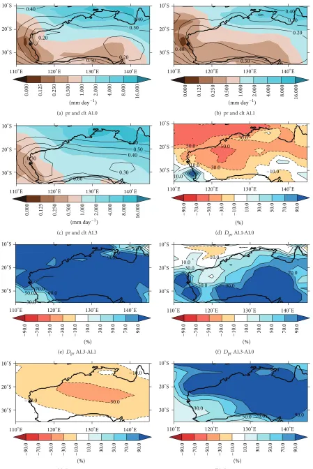
5) for A1.1 relative to A1.0 are also plotted in Figure 9 to investigate this further. The𝐷_SWdnis larger in A1.1 than A1.0 over Western Australia by 5–25 W m−2 around 0930, 1230, and 1530 (Figure 9, column 2), which is consistent with the lower cloud cover fraction in A1.1 (Figure 8(g)). The negative anomaly centred on 140∘E is consistent with a small area of higher surface albedo in A1.1 relative to A1.0; however, over most of the continent there is more absorbed solar radiation in A1.1 relative to A1.0, which should act to warm the low-level atmosphere in A1.1.

The values of𝐷_LWdnare consistently lower in A1.1 relative to A1.0, which suggests that the upwards long-wave radiation is higher in A1.1 (Figure 9, column 3). Increased long-wave emission from the surface should warm the low-level atmosphere more in A1.1 compared to A1.0. Despite the larger upward long-wave radiative flux in A1.1 relative to A1.0, the upward surface sensible and latent heat fluxes are weaker in A1.1 relative to A1.0 at 0930, 1230, and 1530 (Figure 9, columns 4 and 5: positive downward anomalies are indicative of weaker upward values during the day). The large positive 𝐷_Hdnand𝐷_LEdncause the positive𝐷_NETdnaround 0930 and 1230 and are indicative of the soil in A1.1 retaining more of this energy than A1.0. Therefore there is less energy available to heat the lower atmosphere, which causes A1.1 to be cooler at low levels during the day (Figure 4(b)).

At night both the contributions from𝐷_SWdnand 𝐷_LEdn diminish to almost zero whereas𝐷_Hdnreverses from positive to negative by 1830 (Figure 9). The negative𝐷_Hdnand𝐷_LWdn values in A1.1 relative to A1.0 overnight are indicative of the surface acting to warm the lower atmosphere and are consistent with the higher nocturnal temperatures in A1.1 (Figure 4(d)).

(11)

0.000

0.40

0.20

0.50 0.20

0.30 0.40

0.125 0.25 0.500 2.000 8.000

0

1.000 4.000 ₁₆.000

(mm day−1)

110∘_E ₁₂₀∘_E ₁₃₀∘_E ₁₄₀∘_E

10∘_S

20∘S

30∘S

(a) pr and clt A1.0

0.40

0.50

0.20 0.30 0.40

0.000 0.125 0.25 0.500 2.000 8.000

0

1.000 4.000 ₁₆.000

(mm day−1)

110∘E ₁₂₀∘E ₁₃₀∘E ₁₄₀∘E

10∘_S

20∘S

30∘_S

(b) pr and clt A1.1

0.30

0.60 0.30

0.400.50

0.60

0.000 0.125 0.25 0.500 2.000 8.000

0

1.000 4.000 ₁₆.000

(mm day−1)

110∘E 120∘E 130∘E 140∘E

10∘_S

20∘S

30∘_S

(c) pr and clt A1.3

10.0 10.0 50.0

−9

0.0

−7

0.0

−5

0.0

−50.0

−3

0.0

−30.0

−1

0.0

−10.0

10.0 30.0 50.0 70.0 90.0

(%)

110∘E 120∘E 130∘E 140∘E

10∘S

20∘S

30∘_S

(d)𝐷_prA1.1-A1.0

50.070.0

30.0 90.0

90.070.0

50.0

−9

0.0

−7

0.0

−5

0.0

−3

0.0

−1

0.0 _10.0 _30.0 _50.0 _70.0 _90.0

(%)

110∘E 120∘E 130∘E 140∘E

10∘S

20∘_S

30∘S

(e)𝐷_prA1.3-A1.1

50.0 90.0

70.0 30.0

10.0

−9

0.0

−7

0.0

−5

0.0

−3

0.0

−1

0.0

−10.0

10.0 30.0 50.0 70.0 90.0

(%)

110∘E 120∘E 130∘E 140∘E

10∘S

20∘_S

30∘S

(f)𝐷_prA1.3-A1.0

−9

0.0

−7

0.0

−5

0.0

−3

0.0

−30.0

−1

0.0

−10.0

10.0 30.0 50.0 70.0 90.0

(%)

110∘E 120∘E 130∘E 140∘E

10∘S

20∘_S

30∘S

(g)DAcA1.1-A1.0

−9

0.0

−7

0.0

−5

0.0

−3

0.0

−1

0.0 _10.0 _30.0

30.0

50.0 70.0 90.0

90.0

50.0 70.0 90.0

(%)

110∘E ₁₂₀∘E ₁₃₀∘E ₁₄₀∘E

10∘S

20∘_S

30∘_S

[image:11.600.76.525.70.742.2]

(h)DAcA1.3-A1.1

(12)

70.0

30.0

50.0

70.0

−9

0.0

−7

0.0

−5

0.0

−3

0.0

−1

0.0 _10.0 _30.0 _50.0 _70.0 _90.0

(%)

110∘E 120∘E 130∘E 140∘E

10∘S

20∘_S

30∘S

(i)DAcA1.3-A1.0

Figure 8: The climatological mean (1979–2001) DJF precipitation (mm day−1, colored contours) and fractional cloud cover (solid black lines) from (a) A1.0, (b) A1.1, and (c) A1.3. The percentage difference in precipitation for (d) A1.1 relative to A1.0, (e) A1.3 relative to A1.1, and (f) A1.3 relative to A1.0. The percentage change in cloud fraction for (g) A1.1 relative to A1.0, (h) A1.3 relative to A1.1, and (i) A1.3 relative to A1.0.

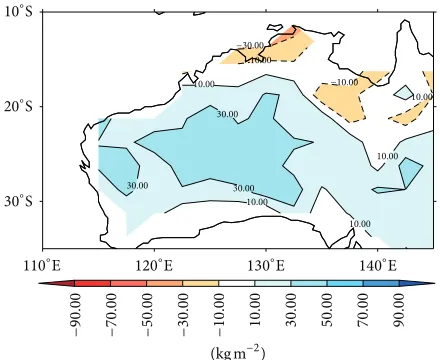
the diurnal temperature range (DTR) in climate models with higher thermal inertia causing a smaller DTR and vice versa. Moreover, they indicate that the thermal inertia is dependent on the soil water content with higher soil water contents corresponding to increased thermal inertia. The differences in the total soil water content over Australia for A1.1 relative to A1.0 are plotted in Figure 10. Despite A1.1 simulating drier conditions at the surface over Australia than A1.0, A1.1 has higher soil moisture contents throughout the depth of the soil (Figure 10), which would result in a higher thermal inertia and a smaller DTR. This is consistent with the lower daytime and higher nocturnal surface air temperatures.

The differences in the diurnal temperature range subse-quently affect the low-level circulation. The reduced surface and low-level air temperatures in A1.1 relative to A1.0 at 1400 AWST act to reduce the amount of dry convection, and therefore convergence, within the heat low. This reduced convergence can be seen in Figure 4(f) at 925–850 hPa. At night, surface cooling causes the nocturnal boundary layer to form, which reduces the low-level drag and causes the increased convergence within the heat low. This is observed at 2000 AWST in A1.0 (see Figures 2(c) and 3(c), described in more detail in [2, 15, 16, 34]); however, the convective mixing will continue for longer in A1.1 as the surface cools slower than in A1.0 between 1400 AWST and 2000 AWST (Figures 7(c) and 7(g)). This causes the low-level drag to be larger in A1.1 than A1.0, which reduces the strength of the flow directed towards the centre of the heat low and causes the weakened convergence (see Figure 4(g)).

4.2. A1.3 Relative to A1.1. Across the whole of Australia, except the far south and west, the atmosphere below 800 hPa is cooler throughout the whole day in A1.3 relative to A1.1 (Figures 5(a)–5(d)). The largest temperature differences (approximately −1.5 K) occur over north Australia at 1400 and 2000 AWST (Figures 5(b) and 5(c)). Nonetheless, the atmosphere above 700 hPa is consistently ∼2 K warmer in A1.3 than in A1.1 (Figures 5(e)–5(h)).

The differences in the DJF-mean precipitation and cloud cover are plotted in Figures 8(e) and 8(h). The change to the PC2 plus “Tripleclouds” cloud scheme (from now PC2T) causes a systematic increase in cloud cover and precipitation over Australia in A1.3 relative to A1.1 and is consistent with the change in the vertical temperature profiles in Figures 5(e)–5(h). The presence of increased cloud acts to reduce the amount of solar radiation reaching the surface, which causes the air temperature to be lower in A1.3 than A1.1 below 800 hPa. Conversely, the increase in latent heating from the presence of the increased cloud cover would act to increase the air temperatures above 700 hPa. Moreover, the largest negative differences in 925 hPa temperatures in A1.3 relative to A1.1 occur where the monsoon precipitation is highest (cf. Figures 5(b) and 5(c) with Figures 8(b) and 8(c)). Therefore, it appears that the inclusion of PC2T has a stronger impact on the local monsoon circulation (and convection) than the heat low.

Overall, the differences between A1.3 and A1.1 are not as strong as the differences between A1.1 and A1.0 at low-levels (below 800 hPa). Above 700 hPa, due to the significant change in cloud physics in A1.3, the opposite is true.

4.3. A1.3 Relative to A1.0. The differences in the circulation and temperature between A1.3 and A1.0 (Figure 6) are a linear combination of the differences between A1.3 relative to A1.1 and A1.1 relative to A1.0 (not shown as the sums of those differences are<10−8). Therefore there is no nonlinear interaction between CABLE1.8 and PC2T physics when they are used together in A1.3.

(13)

105 85

254565 45

0930AWST:D_NETdn

45 8565

25

1230AWST:D_NETdn

45 5 25 −45 −65 −5 −25

1530AWST:D_NETdn

5 −45 −5 −25 −85 −65

1830AWST:D_NETdn

5 −5 −25

2130AWST:D_NETdn

5 −5

−25

0030AWST:D_NETdn

5

0330AWST:D_NETdn

25 5 5

−5

0930AWST:D_SWdn

45 25

5 −5

1230AWST:D_SWdn

25

5

1530AWST:D_SWdn

1830AWST:D_SWdn

2130AWST:D_SWdn

0030AWST:D_SWdn

0330AWST:D_SWdn

−5 −25

0930AWST:D_LWdn

−25 −65 −85 −85

−45 −5

1230AWST:D_LWdn

−105 −5

−85 −65−25

−45

1530AWST:D_LWdn

−5 ₋₅ −85−65

−45 −25

1830AWST:D_LWdn

−5

−25

2130AWST:D_LWdn

−5

−25

0030AWST:D_LWdn

−5

0330AWST:D_LWdn

5 25 105 85 65 45 −5

0930AWST:D_Hdn

5

2545 105 85 65

1230AWST:D_Hdn

5 4525

−5

1530AWST:D_Hdn

5

−5

1830AWST:D_Hdn

5

2130AWST:D_Hdn

5 −5

0030AWST:D_Hdn

−5

0330AWST:D_Hdn

25 ₅

5 −5

0930AWST:D_LEdn

5 5 45

25

1230AWST:D_LEdn

5

5 25 45

1530AWST:D_LEdn

5

1830AWST:D_LEdn

5

2130AWST:D_LEdn

5

0030AWST:D_LEdn

5

0330AWST:D_LEdn

110 ∘E 120 ∘E 13 0 ∘ E 14 0 ∘ E 110 ∘ E 120 ∘ E 13 0 ∘ E 14 0 ∘E 110 ∘ E 120 ∘E 13 0 ∘E 14 0 ∘E 110 ∘E 120 ∘E 13 0 ∘E 14 0 ∘ E 110 ∘ E 120 ∘ E 13 0 ∘ E 14 0 ∘E 110 ∘E 120 ∘E 13 0 ∘ E 14 0 ∘ E 110 ∘ E 120 ∘ E 13 0 ∘ E 14 0 ∘E 110 ∘ E 120 ∘E 13 0 ∘E 14 0 ∘E 110 ∘E 120 ∘E 13 0 ∘E 14 0 ∘ E 110 ∘ E 120 ∘ E 13 0 ∘ E 14 0 ∘E 110 ∘E 120 ∘E 13 0 ∘ E 14 0 ∘ E 110 ∘ E 120 ∘ E 13 0 ∘ E 14 0 ∘E 110 ∘ E 120 ∘E 13 0 ∘E 14 0 ∘E 110 ∘E 120 ∘E 13 0 ∘E 14 0 ∘ E 110 ∘ E 120 ∘ E 13 0 ∘ E 14 0 ∘E 110 ∘E 120 ∘E 13 0 ∘ E 14 0 ∘ E 110 ∘ E 120 ∘ E 13 0 ∘ E 14 0 ∘E 110 ∘ E 120 ∘E 13 0 ∘E 14 0 ∘E 110 ∘E 120 ∘E 13 0 ∘E 14 0 ∘ E 110 ∘ E 120 ∘ E 13 0 ∘ E 14 0 ∘E 110 ∘E 120 ∘E 13 0 ∘ E 14 0 ∘ E 110 ∘ E 120 ∘ E 13 0 ∘ E 14 0 ∘E 110 ∘ E 120 ∘E 13 0 ∘E 14 0 ∘E 110 ∘E 120 ∘E 13 0 ∘E 14 0 ∘ E 110 ∘ E 120 ∘ E 13 0 ∘ E 14 0 ∘E 110 ∘E 120 ∘E 13 0 ∘ E 14 0 ∘ E 110 ∘ E 120 ∘ E 13 0 ∘ E 14 0 ∘E 110 ∘ E 120 ∘E 13 0 ∘E 14 0 ∘E 110 ∘E 120 ∘E 13 0 ∘E 14 0 ∘ E 110 ∘ E 120 ∘ E 13 0 ∘ E 14 0 ∘E 110 ∘E 120 ∘E 13 0 ∘ E 14 0 ∘ E 110 ∘ E 120 ∘ E 13 0 ∘ E 14 0 ∘E 110 ∘ E 120 ∘E 13 0 ∘E 14 0 ∘E 110 ∘E 120 ∘E 13 0 ∘E 14 0 ∘ E 110 ∘ E 120 ∘ E 13 0 ∘ E 14 0 ∘E 10∘_S

20∘_S

30∘_S

10∘S

20∘S

30∘S

10∘S

20∘S

30∘S

10∘S

20∘S

30∘S

10∘S

20∘S

30∘S

10∘S

20∘S

30∘S

10∘_S

20∘_S

30∘_S

10∘_S

20∘_S

30∘_S

10∘_S

20∘_S

30∘_S

10∘_S

20∘_S

30∘_S

10∘_S

20∘_S

30∘_S

10∘S

20∘S

30∘S

10∘S

20∘S

30∘S

10∘S

20∘S

30∘S

10∘S

20∘S

30∘S

10∘_S

20∘_S

30∘_S

10∘S

20∘S

30∘S

10∘S

20∘S

30∘S

10∘S

20∘S 30∘S

10∘S

20∘S 30∘S

10∘S

20∘S

30∘S

10∘_S

20∘S 30∘S

10∘_S

20∘S 30∘S

10∘_S

20∘S

30∘S

10∘_S

20∘S

30∘S

10∘_S

20∘_S

30∘_S

10∘S

20∘S 30∘S

10∘S

20∘S

30∘S

10∘S

20∘S

30∘S

10∘S

20∘S

30∘S

10∘S 20∘_S

30∘S

10∘_S

20∘S 30∘S

10∘S

20∘S 30∘S

10∘S

20∘S 30∘S

10∘S

[image:13.600.54.548.69.754.2]

20∘S 30∘S D

(14)

5 25

25 5 −5

0630AWST:_D_NETdn

5

5 −5

0630AWST:_D_SWdn

−5

0630AWST:_D_LWdn

45 25 5

0630AWST:_D_Hdn

5

0630AWST:_D_LEdn

−105

.0

−9

5.

0

−8

5.

0

−7

5.

0

−6

5.

0

−5

5.

0

−4

5.

0

−3

5.

0

−2

5.

0

−1

5.

0

−5.0 5.0 15.0 25.0 35.0 45.0 55.0 65.0 75.0 85.0 95.0 _105.0

Difference in downward radiative ﬂux (W m−2)

110

∘E

120

∘ E

13

0

∘ E

14

0

∘ E

110

∘E

120

∘E

13

0

∘E

14

0

∘E

110

∘E

120

∘E

13

0

∘ E

14

0

∘ E

110

∘E

120

∘E

13

0

∘E

14

0

∘E

110

∘E

120

∘E

13

0

∘ E

14

0

∘ E 10∘S

20∘S

30∘S

10∘_S

20∘_S

30∘_S

10∘_S

20∘_S

30∘_S

10∘_S

20∘_S

30∘_S

10∘_S

20∘_S

30∘_S

Figure 9: The difference between A1.1 and A1.0 climatological (1979–2001) mean 3-hourly downward radiative fluxes (W m−2) at the surface. Column 1: net radiative flux (𝐷_NETdn); column 2: short-wave radiative flux (𝐷_SWdn); column 3: long-wave radiative flux (𝐷_LWdn); column 4: sensible heat flux (𝐷_Hdn); column 5: latent heat flux (𝐷_LEdn). Time averages are centred on (from row 1 to row 8) 0930 AWST, 1230 AWST, 1530 AWST, 1830 AWST, 2130 AWST, 0030 AWST, 0330 AWST, and 0630 AWST.

cover (see Figures 8(f) and 8(i)). The increased cloud cover also causes the air temperatures above 650 hPa to be warmer in A1.3 relative to A1.0, which resembles the differences between A1.3 and A1.1 and suggests that the differences are driven by using PC2T. Despite the changes in air temperature caused by the different cloud physics in A1.3 relative to A1.1, the changes in circulation around the heat low are much weaker than those caused by changing the surface scheme from MOSES (A1.0) to CABLE1.8 (A1.1). Therefore, in terms of modelling the north-west Australian heat low system, the differences between A1.1 and A1.0 are more significant.

5. Conclusions and Further Work

The aims of this work were to document and discuss the representation of the summertime heat low circulation over north-west Australia in three different configurations of the same GCM (ACCESS). Moreover, this study also aimed at identifying the processes that caused the simulated heat low structure to differ in each simulation.

The main results of this work are as follows:

[image:14.600.318.538.287.467.2]

(i) The differences in the 925 hPa circulation between each configuration of the model are comparable to the differences between each model and the reanalyses (Figure 1).

(ii) The nocturnal convergence into the heat low is stronger in the A1.0 (MOSES) simulation than in A1.1 (CABLE1.8) (Figure 4).

(iii) The low-level atmosphere in A1.0 heats up faster during the day and cools down faster at night than in A1.1 (Figure 7).

(iv) The difference in surface heating and cooling rates between A1.0 and A1.1 appear to be driven by differ-ences in the thermal inertia of the soil used by MOSES and CABLE1.8 (Figures 9 and 10).

(v) The simulated air flow in the north-Australian mon-soon region is more convergent in A1.3 (PC2T) than

−9

0.00

−7

0.00

−5

0.00

−3

0.00

−10.00

−30.00 −10.00

−10.00

10.00 30.00

30.00 30.00

30.00

10.00

10.00 10.00

50.00 70.00 90.00

(kg m−2)

110∘E 120∘E 130∘E 140∘E

10∘_S

20∘S

30∘S

Figure 10: The difference in the total soil moisture content (kg m−2) between A1.1 and A1.0 averaged over all DJFs from 1979 to 2001.

A1.1 (non-PC2T) but there is little impact on the heat low circulation (Figure 5).

(vi) The changes in cloud cover and precipitation in A1.3 relative to A1.1 cause lower air temperatures below 800 hPa and higher air temperatures above 700 hPa (Figure 5).

(vii) The heat low is more sensitive to changes in the surface parameterization (MOSES versus CABLE1.8) than the cloud cover and convection (diagnostic clouds versus PC2T).

(15)

likely to be configured differently in each model. In this study, however, since the parameterized processes were changed individually (and in combination), the impact of changing the surface and cloud schemes on the circulation could be quantified.

The next logical step for this work is to test the hypothesis discussed in Section 4.1 to see whether the larger soil water contents in the A1.1 simulation are responsible for the smaller DTR relative to A1.0. If reducing the soil water content in A1.1 results in an increase in the DTR such that it becomes almost identical to that of A1.0, then the result would imply that the amount of water stored in the soil is more important in determining the interaction between the land surface and the lower atmosphere than the configuration of the surface scheme employed. This would allow model developers to target the representation of subsurface soil moisture properties as a priority in arid and semiarid land areas such as north-west Australia.

Conflict of Interests

The authors declare that there is no conflict of interests regarding the publication of this paper.

Acknowledgments

Both Matthew M. Allcock and Duncan Ackerley were sup-ported by the ARC Centre of Excellence for Climate Sys-tem Science (CE110001028). The ACCESS simulations were undertaken with the assistance of resources from the National Computational Infrastructure (NCI), which is supported by the Australian Government. Finally, ERA-Interim reanalysis data were supplied by the European Centre for Medium-Range Weather Forecasts.

References

[1] Z. R´acz and R. K. Smith, “The dynamics of heat lows,”Quarterly Journal of the Royal Meteorological Society, vol. 125, no. 553, pp. 225–252, 1999.

[2] T. Spengler, M. J. Reeder, and R. K. Smith, “The dynamics of heat lows in simple background flows,”Quarterly Journal of the Royal Meteorological Society, vol. 131, no. 612, pp. 3147–3165, 2005.

[3] S. J. Arnup and M. J. Reeder, “The diurnal and seasonal variation of the northern Australian dryline,”Monthly Weather Review, vol. 135, no. 8, pp. 2995–3008, 2007.

[4] S. J. Arnup and M. J. Reeder, “The structure and evolution of the northern Australian dry line,”Australian Meteorological and Oceanographic Journal, vol. 58, no. 4, pp. 215–231, 2009.

[5] G. Berry, M. J. Reeder, and C. Jakob, “Physical mechanisms regulating summertime rainfall over Northwestern Australia,” Journal of Climate, vol. 24, no. 14, pp. 3705–3717, 2011.

[6] A. Uriate, “Rainfall on the Northern coast of the Iberian peninsula,”Journal of Meteorology, vol. 5, pp. 138–144, 1980.

[7] M. A. Gaertner, C. Fernandez, and M. Castro, “A two-dimensional simulation of the Iberian summer thermal low,” Monthly Weather Review, vol. 121, no. 10, pp. 2740–2756, 1993.

[8] S. Alonso, A. Portela, and C. Ramis, “First considerations on the structure and development of the Iberian thermal low-pressure system,”Annales Geophysicae, vol. 12, no. 5, pp. 457–468, 1994. [9] A. Portela and M. Castro, “Summer thermal lows in the Iberian

peninsula: a three-dimensional simulation,”Quarterly Journal of the Royal Meteorological Society, vol. 122, no. 529, pp. 1–22, 1996.

[10] C. S. Ramage, Monsoon Meteorology, Academic Press, New York, NY, USA, 1971.

[11] D. E. Pedgley, “Desert depressions over North-East Africa,”The Meteorological Magazine, vol. 101, pp. 228–244, 1972.

[12] J. F. Griffiths and K. H. Soliman, “The northern desert,” inWorld Survey of Climatology, Vol. 10, Climates of Africa, J. F. Griffiths, Ed., pp. 75–111, Elsevier, 1972.

[13] D. J. Parker, R. R. Burton, A. Diongue-Niang et al., “The diurnal cycle of the West African monsoon circulation,” Quarterly Journal of the Royal Meteorological Society, vol. 131, no. 611, pp. 2839–2860, 2005.

[14] R. Suppiah, “The Australian summer monsoon: a review,” Progress in Physical Geography, vol. 16, no. 3, pp. 283–318, 1992. [15] D. Ackerley, G. Berry, C. Jakob, and M. J. Reeder, “The roles of diurnal forcing and large-scale moisture transport for initiating rain over northwest Australia in a GCM,”Quarterly Journal of the Royal Meteorological Society, vol. 140, no. 685, pp. 2515–2526, 2014.

[16] D. Ackerley, G. Berry, C. Jakob, M. J. Reeder, and J. Schwendike, “Summertime precipitation over northern Australia in AMIP simulations from CMIP5,”Quarterly Journal of the Royal Mete-orological Society, vol. 141, no. 690, pp. 1753–1768, 2015. [17] T. Keenan, K. Puri, T. Hirst et al., “Next generation Australian

community climate and earth-system simulator (NG-ACCESS) a Roadmap 2014–2019,” CAWCR Technical Report 075, Bureau of Meteorology, Melbourne, Australia, 2014, http://www.cawcr .gov.au/publications/technicalreports/CTR 075.pdf.

[18] K. Puri, G. Dietachmayer, P. Steinle et al., “Implementation of the initial ACCESS numerical weather prediction system,” Australian Meteorological and Oceanographic Journal, vol. 63, no. 2, pp. 265–284, 2013.

[19] D. Bi, M. Dix, S. J. Marsland et al., “The ACCESS coupled model: description, control climate and evaluation,”Australian Meteorological and Oceanographic Journal, vol. 63, no. 1, pp. 41– 64, 2013.

[20] T. Davies, M. J. P. Cullen, A. J. Malcolm et al., “A new dynamical core of the Met Office’s global and regional modelling of the atmosphere,”Quarterly Journal of the Royal Meteorological Society, vol. 131, no. 608, pp. 1759–1782, 2005.

[21] G. M. Martin, N. Bellouin, W. J. Collins et al., “The HadGEM2 family of Met Office Unified Model climate configurations,” Geoscientific Model Development, vol. 4, no. 3, pp. 723–757, 2011. [22] E. A. Kowalczyk, Y. P. Wang, R. M. Law, H. L. Davies, J. L. McGre-gor, and G. Abramowitz, “The CSIRO atmosphere biosphere land exchange (CABLE) model for use in climate models and as an offline model,” Marine and Atmospheric Research Paper 013, CSIRO, Clayton South, Australia, 2006, http://www.cmar.csiro .au/e-print/open/kowalczykea 2006a.pdf.

[23] E. A. Kowalczyk, L. Stevens, R. M. Law et al., “The land surface model component of ACCESS: description and impact on the simulated surface climatology,”Australian Meteorological and Oceanographic Journal, vol. 63, no. 1, pp. 65–82, 2013.

(16)

1D Radiation schemes by using three regions at each height,” Journal of Climate, vol. 21, no. 11, pp. 2352–2370, 2008. [25] Z. Sun, C. Franklin, X. Zhou et al., “Modifications in

atmo-spheric physical parameterization for improving SST simula-tion in the ACCESS coupled model,”Australian Meteorological and Oceanographic Journal, vol. 63, no. 1, pp. 233–247, 2013. [26] R. N. B. Smith, “A scheme for predicting layer clouds and their

water content in a general circulation model,”Quarterly Journal Royal Meteorological Society, vol. 116, no. 492, pp. 435–460, 1990. [27] D. R. Wilson, R. N. B. Smith, D. Gregory, C. Wilson, A. C. Bushell, and S. Cusack, “The large-scale cloud scheme and saturated specific humidity,” Unified Model Documentation Paper 26, Met Office, Exeter, UK, 2004.

[28] D. R. Wilson, A. C. Bushell, A. M. Kerr-Munslow, J. D. Price, and C. J. Morcrette, “PC2: a prognostic cloud fraction and condensation scheme. I. Scheme description,”Quarterly Journal of the Royal Meteorological Society, vol. 134, no. 637, pp. 2093– 2107, 2008.

[29] D. R. Wilson, A. C. Bushell, A. M. Kerr-Munslow, J. D. Price, C. J. Morcrette, and A. Bodas-Salcedo, “PC2: a prognostic cloud fraction and condensation scheme. II: climate model simulations,” Quarterly Journal of the Royal Meteorological Society, vol. 134, no. 637, pp. 2109–2125, 2008.

[30] C. N. Franklin, C. Jakob, M. Dix, A. Protat, and G. Roff, “Assessing the performance of a prognostic and a diagnostic cloud scheme using single column model simulations of TWP-ICE,”Quarterly Journal of the Royal Meteorological Society, vol. 138, no. 664, pp. 734–754, 2012.

[31] W. L. Gates, “AMIP: the Atmospheric Model Intercomparison Project,”Bulletin of the American Meteorological Society, vol. 73, no. 12, pp. 1962–1970, 1992.

[32] W. L. Gates, J. S. Boyle, C. Covey et al., “An overview of the results of the Atmospheric Model Intercomparison Project (AMIP I),”Bulletin of the American Meteorological Society, vol. 80, no. 1, pp. 29–55, 1999.

[33] D. P. Dee, S. M. Uppala, A. J. Simmons et al., “The ERA-Interim reanalysis: configuration and performance of the data assim-ilation system,”Quarterly Journal of the Royal Meteorological Society, vol. 137, no. 656, pp. 553–597, 2011.

[34] T. Spengler and R. K. Smith, “The dynamics of heat lows over flat terrain,”Quarterly Journal of the Royal Meteorological Society, vol. 134, no. 637, pp. 2157–2172, 2008.

(17)