State bounds estimation for nonlinear systems using μ-analysis

This is a repository copy of State bounds estimation for nonlinear systems using

μ-analysis.

White Rose Research Online URL for this paper:

http://eprints.whiterose.ac.uk/144678/

Version: Accepted Version

Proceedings Paper:

Kim, J orcid.org/0000-0002-3456-6614, Kishida, M and Bates, DG (2016) State bounds

estimation for nonlinear systems using μ-analysis. In: IFAC Proceedings Volumes. 19th

IFAC World Congress, 24-29 Aug 2014, Cape Town, South Africa. Elsevier , pp.

1661-1666. ISBN 9783902823625

https://doi.org/10.3182/20140824-6-ZA-1003.01572

© 2014, Elsevier. This manuscript version is made available under the CC-BY-NC-ND 4.0

license http://creativecommons.org/licenses/by-nc-nd/4.0/.

[email protected] https://eprints.whiterose.ac.uk/

Reuse

This article is distributed under the terms of the Creative Commons Attribution-NonCommercial-NoDerivs (CC BY-NC-ND) licence. This licence only allows you to download this work and share it with others as long as you credit the authors, but you can’t change the article in any way or use it commercially. More

information and the full terms of the licence here: https://creativecommons.org/licenses/

Takedown

If you consider content in White Rose Research Online to be in breach of UK law, please notify us by

State bounds estimation for nonlinear

systems using

µ

-analysis

⋆

Jongrae Kim∗

Masako Kishida∗∗

Declan G. Bates∗∗∗

∗

Biomedical Engineering/Aerospace Sciences, University Avenue, University of Glasgow, Glasgow G12 8QQ, UK (e-mail:

[email protected]). ∗∗

Electrical & Computer Engineering, University of Canterbury, Christchurch, New Zealand (e-mail: [email protected]) ∗∗∗

School of Engineering, University of Warwick, Coventry CV4 7AL, UK (e-mail: [email protected])

Abstract:Developing state bound estimation algorithms for nonlinear systems has been of high importance in robustness analysis of dynamic systems. For many cases, Monte-Carlo simulation might be the only tool to estimate these bounds for a general type of nonlinear systems. The required number of simulations for a tight bound, however, would be very large and it might be impossible to complete within a given computation time. µ-formulation for state bounds transforms the bound estimation problem to a singularity problem and the singular problem is solved using a randomised optimisation approach. The performance of the algorithms are demonstrated by a simple discrete system; large-scale biological systems; and a hybrid system.

Keywords:State bound estimation, Nonlinear discontinuous system

1. INTRODUCTION

Robustness analysis is an indispensable step in designing engineering systems (Balas et al., 2001; Ferreres and Biannic, 2001; Menon et al., 2006). It is also accepted now one of the most important aspects in analysing biological systems (Kitano, 2004; Wagner, 2005; Gilchrist et al., 2006; Kim et al., 2006; Shinar et al., 2007; Clodong et al., 2007; Acar et al., 2008). Systematic approach to model biological interactions and analyse measurement data is one of the highly preferable ways in improving our understanding of complex systems (Kholodenko et al., 2002; Hoehndorf et al., 2011). Recently, some of the models are described with many states and parameters of several hundreds (Kuhn et al., 2009; Chen et al., 2009) and these provide information that was not available with small scale models. Similarly, current engineering systems become more and more complex and this tendency will continue in future. Hence, it is important to have an efficient numerical methods to analyse these large-scale systems.

Structured singular value or µ-analysis has been one of the most successful tools for robustness evaluation (Doyle, 1982; Skogestad and Postlethwaite, 1996; Kao et al., 2001; Cantoni and Glover, 2000). Even though the computa-tional complexity of µ-analysis was acknowledged, it has been successfully used for many practical systems design and analyses.

The computational complexity proof in Braatz et al. (1994) is performed by transforming µ problem to a cor-responding optimisation problem that is known to be

NP-⋆ _{This research was supported by EOARD (European Office of} Aerospace Research & Development), the grant number US-EURO-LO (FA8655-13-1-3029).

hard. As far as NP6=P, the computational complexity is a fundamental obstacle that cannot be overcome by any traditional algorithms. However, practicallyµ-analysis al-gorithm produced many useful results and recently, it is further extended to solve some class of optimisation prob-lems efficiently (Kishida et al., 2011). This is an inverse interpretation of the formulation in Braatz et al. (1994). The application in Kishida et al. (2011) is calculating state bounds for polynomial nonlinear discrete systems, where initial states and parameters in the systems are given with known uncertain bounds. Then, the state maximum and minimum bounds are calculated usingµupper and lower bounds algorithms. As long as the nonlinearity appears in polynomial formats, the uncertainties can be decoupled from the known parts and the system can be described in Linear Fractional Transformation (LFT) (Braatz et al., 1994; Doyle et al., 1989). Once it is in LFT form, then there are some powerful numerical tools that provide the upper and the lower bounds ofµ(Balas et al., 2001).

non-smooth nonlinear functions using a random sampling method (Zhao et al., 2011).

This paper is organised as follows: Firstly, state bounds estimation problem is formulated as LFT-free µ-analysis. Secondly, state worst-bounds algorithms are presented. Thirdly, the algorithm is parallelised to run on GPU (Graphical Processing Unit) and its performance is demon-strated using three examples: an oscillatory discrete sys-tem; a large-scale biological system and a hybrid system. Finally, the conclusions are presented.

2. STATE BOUNDS IN LFT-FREEµ-FORMULATION

A nonlinear dynamical system is given by ˙

x=f(x, p), (1)

where the initial conditions are x0 =x(0), ˙x is the time-derivative of x, x is the state vector, an element of the set, Rnx, Rnx is the n

x-dimensional real space, nx is a

positive integer,pis the uncertain parameters, an element ofRnp,n

p is a positive integer, and f(x, p) is a nonlinear

function in x and p including dis-continuous functions and non-smooth functions. For the well-posedness of the problem, f(x, p) is assumed to give a unique solution for the nonlinear differential equation. For a chosen positive real number, ∆t, a transition function φ(,) is defined to satisfy the following:

xk+1=φ(xk, p) (2)

wherexk=x(k∆t) fork= 0,1,2, . . .. The problem is

find-ing the worst-bounds for the maximum and the minimum of the state,xk+1, for the given bounds forx0 andp. For brevity, we consider a scalar case forxandponly but the general formulation for the multi-dimensional x and pis exactly the same as shown in below.

Problem 1. (state bounds estimation) Calculate φ_min, ¯

φmin,φ_maxand ¯φmax in the following inequalities:

φ_min≤φ≤φ¯min, (3a)

φ_max≤φ¯≤φ¯max, (3b)

where φ≤φ(xk, p)≤φ,¯ x0≤x0≤x¯0, p≤p≤p, and all¯ the upper and the lower bounds forφ(xk, p),x0andpare finite.

By solving problem 1 we are to find state boundaries for xk+1 for the give uncertain values for the initial condition and the parameters in the dynamical system. A special case of the problem, where φis a polynomial function in xk andp, can be transformed into LFT form and existing

µ bounds algorithms can be directly used to obtain the bounds. Details about the special case can be found in Kishida et al. (2011). Although Problem 1 is more general than the one in Kishida et al. (2011), the main idea obtaining the state bounds usingµ-formulation is the same but exploiting the LFT-free formulation in Zhao et al. (2011), which will be presented in the following.

Consider the case that eachx0andpcan be written as

x0=xc+wxδx (4a)

p=pc+wpδp (4b)

where xc = (x0+ ¯x0)/2,pc = (p+ ¯p)/2, and wx orwp is

a weight to define the boundary ofx0orpsuch thatδxor

δp is given by

1

1

1

0

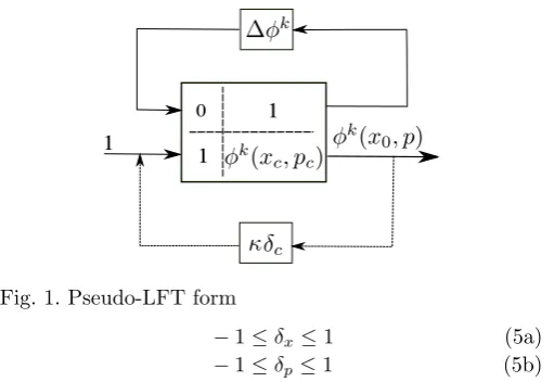
Fig. 1. Pseudo-LFT form

−1≤δx≤1 (5a)

−1≤δp≤1 (5b)

In order to lift the polynomial function requirement on φ(xk, p), define

∆φk(δx, δp) :=φk(x0, p)−φk(xc, pc) (6)

where

φk₍

·, p) :=φ◦φ◦φ◦. . .◦φ

| {z }

k-times

(·, p) (7)

and

φ2

(·, p) =φ◦φ(·, p) =φ[φ(·, p), p] (8) Now, a pseudo-LFT form as shown in Figure 1 is to be constructed. It is called a pseudo-LFT as it is in the LFT format but it can be only evaluated for a fixedδxandδp. In

the standard LFT-formulation, ∆φk _{is a constant matrix}

with a structure. On the other hand, in the pseudo-LFT formulation, it is a varying vector depending on the values ofδx andδp.

From the pseudo-LFT shown in Figure 1 and the equiv-alency between µ-bounds and the optimisation problem shown in Braatz et al. (1994), the maximum of|φk_(x

0, p)| is bounded above as

max|φk_(x

0, p)| ≤ 1

κ∗ (9)

where κ∗

is the minimum κ among the ones satisfy the singular condition:

|I2−N∆|= 0, (10)

| · | is the determinant of matrix, I2 is the 2×2 identify matrix,

N =

0 1

1 φk(xc, pc)

, (11a)

∆ =

∆φk ₀

0 κδc

, (11b)

|δc|=|δR+δIj| ≤1,δRandδI are the real numbers whose

magnitude is less than or equal to 1, andj=√−1.

The singularity condition is expanded

|I2−N∆|=

1 −κδc

−∆φk ₁

−κφk_(x c, pc)δc

= 1−κφk_(x

c, pc)δc−κ∆φkδc

=1−κφk_(x

c, pc) + ∆φk

δR

−κφk_(x

c, pc) + ∆φk

δIj= 0 (12)

19th IFAC World Congress

Cape Town, South Africa. August 24-29, 2014

singular point r

r

r

r

r

r -r

-r -r

-r -r

-r

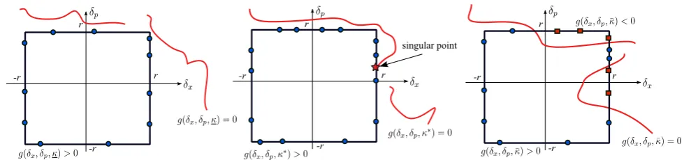
Fig. 2. Sign changes along the uncertain box boundary: asκis smaller thanκ∗

, all signs ofg(δx, δp, κ) for the samples

at the boundary are positive; on the other hand, when ¯κ is greater thanκ∗

, there are red box samples and blue circle samples whose sign ofg(δx, δp,κ) is positive and negative, respectively.¯

The following is the only singular condition: 1−κφk_(x

c, pc) + ∆φk

δR= 0, andδI = 0 (13)

i.e., the imaginary value of δc is always equal to zero.

Notice also thatφk_(x

c, pc) + ∆φk is equal toφk(x0, p) by the definition. Therefore, the minimum κ, i.e. κ∗

, occurs at the following condition:

κ∗

= 1

max[φk_(x

0, p)δR]

= 1

max|φk_(x

0, p)|

(14)

whereδR=±1. This looks trivial and it does not seem to

help to find the bounds forφk_(x

0, p). In the next section, a random sampling approach to solve the above problem, which could be interpreted as a multi-dimensional bi-section method.

3. WORST BOUNDS ESTIMATION

Define

g(δx, δp, κ) := 1−κ|φk(xc+Wxδx, pc+Wpδp)| (15)

where −r ≤δx ≤r, −r ≤δp ≤r, κ >0, and r∈ (0,1].

Note thatg(·,·,·) could be dis-continuous asφk₍

·,·) could be dis-continuous. As shown in Figure 2, if ¯κis larger than κ∗

, then there are two cases, i.e. either having two types of samples, whose signs are positive or negative, or having one type of sample, whose signs are all negative. Similarly, if only positive signs are found, then the corresponding κ is smaller than κ∗

, which is the case that κ=κ. Hence, the bound forκ∗

is given by κ≤κ∗

≤κ¯ (16)

where ¯κis a deterministic bound as we found the negative sign butκis probabilistic as it has always some danger to be failed depending on the number of samples checked on the boundary.

Algorithm 1. Pre-κestimation

(1) Set N, the number of samples along the face of the uncertain box shown in Figure 2

(2) Set the initial boundary for κsuch that ǫ≤κ∗ ≤E, where ǫ is equal to zero and E could be the largest number that can be expressed in computer.

(3) Set the tolerance,ε, for the magnitude of the interval, [ǫ, E], i.e.E−ǫ

(4) Set κ= (ǫ+E)/2, which is the initial guess of ¯κ. (5) for i= 1 toN

• Evaluate g(δx, δp, κ) for the giveni-th sample of

δk andδp

• ifg(δx, δp, κ)<0, then replaceE byκand break

the for-loop, else continue the for-loop

(6) Ifi=N and g(δk, δp, κ) for all samples are positive,

then replaceǫbyκ.

(7) IfE−ǫ is smaller than ε, then declare κp =E and

stop. Otherwise, go to step 4)

Note that κp from the pre-κ estimation algorithm does

not need to be tight as long as it is smaller thanκ∗ . The reason to calculate κp using the above algorithm before

actually obtaining any tight bounds for φk_(x

0, p) is that the value ofφk_(x

0, p) can be positive and negative and the definition of κ∗

in (14) is given in terms of the absolute value ofφk_(x

0, p).

In order to estimate the bounds for the maximum φk_(x

0, p), the following is defined:

¯

g(δx, δp, κ) := 1−κ|φk(x0, p) +s/κ_p| (17) where s is a safety factor, greater than 1. As 1/κp >

|φk_(x

0, p)|can be guaranteed only in a probabilistic sense, the safety factor will make sure the terms inside the abso-lute sign be positive. Then, the maximum of|φk_(x

0, p) + s/κp|occurs at ¯φk(x0, p) +s/κ.

Algorithm 2. φ-bounds estimation Algorithm¯

(1) Run the pre-κ estimation algorithm after replacing g(δx, δp, κ) by ¯g(δx, δp, κ)

(2) Setκ=ǫand ¯κ=E

(3) Declareφ_max= 1/¯κ−s/κp and ¯φmax= 1/κ−s/κp

Similarly, to obtain the bounds for the minimum, define g(δx, δp, κ) := 1−κ|φk(x0, p)−s/κp| (18)

and run the following algorithm:

Algorithm 3. φ-bounds estimation Algorithm

(1) Run the pre-κ estimation algorithm after replacing g(δx, δp, κ) byg(δx, δp, κ)

(2) Setκ=ǫand ¯κ=E

(3) Declareφ_min= 1/¯κ+s/κp and ¯φmin= 1/κ+s/κp

0 5 10 15 20 25 30 35 40

−2 −1.5 −1 −0.5

0 0.5 1 1.5 2

k

x 1,k

Maximum bound Minimum bound

Monte₋Carlo Simulations

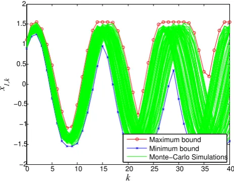
Fig. 3. Bounds forx1,k

Remark 2. The total computational cost depends on how many times the algorithms are executed for different rin (0,1]. If the upper bounds could be provided with less computation, the proposed algorithm could be used only for finding lower bounds.

The proposed three algorithms are embarrassingly par-allel, i.e. all sampling evaluations are independent each other and no effort is required to parallelise the algo-rithms. Therefore, it is a perfect problem to be solved on GPU (Graphical Processing Unit). The algorithms are im-plemented using CUDA-GPU (NVIDIA Developer zone: NVIDIA, CUDA 5.0, 2013). In the following examples, the sampling evaluation part of the algorithms is running on NVIDIA Tesla C2050, which has 449 Cores and the maximum number of threads per block is 1024.

4. EXAMPLES

4.1 Oscillatory state

The following example is from Kishida et al. (2011):

x1,k+1 x2,k+1

=φ(xk, p) =

1

p

1 +p2

1 p

−p 1 x1,k

x2,k

(19)

Because of the polynomial format requirement of the algo-rithm in Kishida et al. (2011),p1 +p2

c was used instead of

p

1 +p2_{. Here, it does not need to be polynomial and the} original form,p1 +p2_{, is used. The intervals for the initial} state and the uncertain parameters,p, are given as follows: 0.9≤x0,1≤1.1, 0.9≤x0,2≤1.1, and 0.45≤p≤0.55. The algorithm firstly calculates the pre upper bound for |φ|, 1/κ, and sets= 2. Secondly, the bounds for max(φ) and min(φ) are obtained by the algorithm 2 and 3. Figure 3 shows the bounds for x1,k, where k = 1,2, . . . ,39,40.

The upper and lower bounds of the maximum and the minimum for r = 1 shown in Figure 3 are very close to each other. All trajectories from random simulations are well bounded by the estimated bounds.

4.2 ErbB Signalling Pathways

ErbB or epidermal growth factor receptor related path-ways are among the most extensively studied biological

0 5 10 15 20 25 30

0 10 20 30 40 50 60 70 80 90 100

time [minutes]

p−ErbB1

[norma

lised]

Maximum bound Minimum bound Monte−Carlo Simulations

Fig. 4. Bounds for p-ErbB1 with respect to uncertainties in 226 kinetic parameters

signalling networks (Chen et al., 2009). Abnormality of ErbB signalling pathways cause various human cancers (Engelman et al., 2007; Zhou et al., 2009; Yonesaka et al., 2011). In Chen et al. (2009), an ErbB mathematical model including 13 known ErbB ligands, EGF (Epidermal Growth Factor) and heregulin (HGF) and Erk and Akt pathways are presented. It has 504 states, 828 reactions and 226 kinetic parameters. The set of 504 differential equations is extracted from the simbiology model (Chen et al., 2009). It is known that this model is only valid up to a few hours and it is not necessary for this system to be stable for infinite time period. As long as the states remain in a certain bound, the network works perfectly as it should be. Hence, the required robustness analysis is obtaining the future state bounds with respect to the uncertain parameters.

One of the interesting biological features found in Chen et al. (2009) using the model is that parametric sensitiv-ities of the dynamical system strongly depend on input condition. This could be the reason that it provides so diverse responses. Parametric uncertainties are introduced for those 226 kinetic parameters. The uncertainty ranges

are set to ±10% from the nominal values. Among the

several input conditions, the robustness is tested for the case of EGF equal to 5nM. The bounds for phospholilated ErbB1, i.e. p-ErbB1, is shown in Figure 4. Again, the up-per and lower bounds for the maximum and the minimum are very close to each other and only the upper bounds for both are indicated. All trajectories from random simula-tions are well bounded by the estimated bounds.

4.3 Inverted Pendulum: Hybrid System

A switching controller for inverted pendulum stabilisation is shown in ˚Astr¨om and Furuta (2000). A simplified version of the system is given by

¨

θ=psinθ−ucosθ (20)

where θ is the angle of pendulum measured from the

upright position, p is the uncertainty caused by some physical parameters anduis the control input. The total energy,E, including kinetic and potential energy is given by

19th IFAC World Congress

Cape Town, South Africa. August 24-29, 2014

0 1 2 3 4 5 6 7 8 9 10 0

1 2

time [s]

C

ont

rol

le

r P

ha

se

Fig. 5. Controller switching phase examples: 0 for waiting; 1 for the energy dissipation control; and 2 for feedback linearisation control.

E= 1 2θ˙

2

+ (cosθ−1)

The controller proposed in ˚Astr¨om and Furuta (2000) has the following switching behaviours:

• Energy dissipation phase(phase 1): if|E|> ǫ, where ǫis a positive real number, then

u= sign(E) ˙θ 1 +|θ˙|

• Waiting phase(phase 0): if|E| ≤ǫand|θ˙|+|θ|> δ, u= 0

• Feedback linearisation control phase (phase 2): if |E| ≤ǫand|θ˙|+|θ| ≤δ,

u= 2 ˙θ+θ+ sinθ cosθ

The ranges for the initial values are set to: |θ(0)| ≤ 19◦ , |θ(0)˙ | ≤20◦

/s, the uncertainty range is given by 0.1≤p≤ 1.9, i.e.±90% uncertainty from the nominal value, 1, and ǫandδ are set to 0.1 and 0.8, respectively.

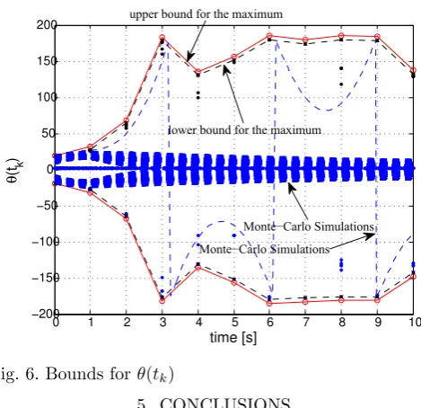
An example of the controller phase switching history is shown in Figure 5. The system dynamics is highly nonlinear because of its inherent nonlinearities and the switching control. The estimated bounds are shown in Figure 6. Although it only requires to calculate the bounds for one of either sign as the system is symmetric, for the demonstration purpose, both bounds are calculated. At t = 10s, the bounds are between ±140◦

but most of the trajectories found by Monte-Carlo simulations converge to zero. In fact, the Monte-Carlo simulation method finds only one trajectory but still far from the bound att= 10s. This clearly demonstrates the advantage of the proposed bound algorithm over the blind Monte-Carlo simulations. The number of samples, N, for this example is set to 1024x10 and the one for Monte-Carlo simulations is twice more thanN used. The calculation time of the presented algorithm for each instance is less than 0.5s. Monte-Carlo simulations takes significantly longer time, about 3 minutes, which would be varying depending on the number of samples, and cannot find any solution closer to the lower bounds att= 10s.

0 1 2 3 4 5 6 7 8 9 10

−200 −150 −100 −50

0 50 100 150 200

time [s]

θ

(tk

)

upper bound for the maximum

lower bound for the maximum

Monte−Carlo Simulations Monte−Carlo Simulations

Fig. 6. Bounds forθ(tk)

5. CONCLUSIONS

An algorithm for calculating state bounds for general non-linear systems with uncertain initial states and parameters are developed, which combinesµ-formulation for optimi-sation problem and pseudo-LFT format. The algorithms have several advantages including: 1) no effort to obtain an LFT form is required, 2) easy to parallelise on distributed computers, and 3) the algorithm is, in fact, applicable to many types of functions including the one having finite number of discontinuity. The algorithms are applied to a simple oscillatory nonlinear discrete system, a high-dimensional biological model for ErbB signalling path-ways, and a hybrid system. It is highly desirable to have numerically efficient algorithms to estimate state bounds for general nonlinear systems. Especially, the input-output robustness analysis with respect to various parametric perturbations are one of the main interest in the robustness of biological networks; Unmanned Aerial Vehicle operating in uncertain environment requires to predict the future state bounds in order to plan or re-plan its behaviour; Predicting a group of space debris is very important for the safety of any space mission. The suggested algorithm could be the main tool to analyse such complex nonlinear systems with uncertainties.

ACKNOWLEDGEMENTS

Effort sponsored by the Air Force Office of Scientific Research, Air Force Material Command, USAF, under grant number FA8655-13-1-3029. The U.S Government is authorized to reproduce and distribute reprints for Gov-ernmental purpose notwithstanding any copyright nota-tion thereon. The authors would like to thank Lt. Col. Kevin Bollino of US-Air Force Research Laboratory for his support.

REFERENCES ˚

Astr¨om, K.J. and Furuta, K. (2000). Swinging up a

pendulum by energy control. Automatica, 36(2), 287– 295. doi:10.1016/s0005-1098(99)00140-5.

environments. Nature Genetics, 40(4), 471–475. doi: 10.1038/ng.110. PMID: 18362885.

Balas, G.J., Doyle, J.C., Glover, K., Packard, A., and Smith, R. (2001). µ-Analysis and Synthesis Toolbox: For Use with MATLAB, User’s Guide, Version 3. The MathWorks, Inc.

Braatz, R., Young, P., Doyle, J., and Morari, M. (1994). Computational complexity ofµ calculation. Automatic Control, IEEE Transactions on, 39(5), 1000 –1002. doi: 10.1109/9.284879.

Cantoni, M. and Glover, K. (2000). Gap-metric robustness analysis of linear periodically time-varying feedback systems. SIAM Journal on Control and Optimization, 38(3), 803–822.

Chen, W.W., Schoeberl, B., Jasper, P.J., Niepel, M., Nielsen, U.B., Lauffenburger, D.A., and Sorger, P.K. (2009). Input-output behavior of ErbB signaling path-ways as revealed by a mass action model trained against

dynamic data. Molecular Systems Biology, 5. doi:

10.1038/msb.2008.74.

Clodong, S., Dhring, U., Kronk, L., Wilde, A., Axmann, I., Herzel, H., and Kollmann, M. (2007). Functioning and robustness of a bacterial circadian clock. Molecular Systems Biology, 3, 90. doi:10.1038/msb4100128. PMID: 17353932.

Doyle, J. (1982). Analysis of feedback systems with struc-tured uncertainties. IEEE Transactions on Aerospace and Electronic Systems, 129(6), 242–250.

Doyle, J.C., Glover, K., Khargonekar, P.P., and Francis, B.A. (1989). State-space solutions to standard h2 and h∞control problems. IEEE Transactions on Automatic Control, 34(8), 831–847.

Engelman, J.A., Zejnullahu, K., Mitsudomi, T., Song, Y., Hyland, C., Park, J.O., Lindeman, N., Gale, C.M., Zhao, X., Christensen, J., Kosaka, T., Holmes, A.J., Rogers, A.M., Cappuzzo, F., Mok, T., Lee, C., Johnson, B.E., Cantley, L.C., and Jnne, P.A. (2007). Met amplification leads to gefitinib resistance in lung cancer by activating erbb3 signaling. Science, 316(5827), 1039–1043. doi: 10.1126/science.1141478.

Ferreres, G. and Biannic, J.M. (2001). Reliable compu-tation of the robustness margin for a flexible aircraft. Control Engineering Practice, 9, 1267–1278.

Gilchrist, M., Thorsson, V., Li, B., Rust, A.G., Korb, M., Kennedy, K., Hai, T., Bolouri, H., and Aderem, A. (2006). Systems biology approaches identify ATF3 as a negative regulator of toll-like recepter 4. Nature, 441(11), 173–178.

Hoehndorf, R., Dumontier, M., Gennari, J.H.,

Wimalaratne, S., de Bono, B., Cook, D.L., and

Gkoutos, G.V. (2011). Integrating systems biology

models and biomedical ontologies. BMC systems

biology, 5(1), 124+. doi:10.1186/1752-0509-5-124. Kao, C.Y., Megretski, A., and J¨onsson, U.T. (2001).

A cutting plane algorithm for robustness analysis of periodically time-varying system. IEEE Transactions on Automatic Control, 46(4), 579–592.

Kholodenko, B.N., Kiyatkin, A., Bruggeman, F.J., Sontag, E., and Westerhoff, H.V. (2002). Untangling the wires: A strategy to trace functional interactions in signaling and gene networks.Proceedings of the National Academy of Sciences, 99(20), 12841–12846.

Kim, J., Bates, D., and Postlethwaite, I. (2009). A

geometrical formulation of the mu-lower bound problem. IET Control Theory & Applications, 3(4), 465–472. doi: 10.1049/iet-cta.2007.0391.

Kim, J., Bates, D.G., Postlethwaite, I., Ma, L., and Igle-sias, P. (2006). Robustness analysis of biochemical networks models. IEE Systems Biology, 153(3), 96–104. Kishida, M., Rumschinski, P., Findeisen, R., and Braatz, R.D. (2011). Efficient polynomial-time outer bounds on state trajectories for uncertain polynomial systems using skewed structured singular values. InIEEE Multi-Conferences on Systems and Control. Denver, CO., USA.

Kitano, H. (2004). Biological robustness. Nat Rev Genet, 5(11), 826–837. doi:10.1038/nrg1471.

Kuhn, C., Wierling, C., Kuhn, A., Klipp, E., Panopoulou, G., Lehrach, H., and Poustka, A. (2009). Monte Carlo analysis of an ODE Model of the Sea Urchin Endomeso-derm Network. BMC Systems Biology, 3(1), 83+. doi: 10.1186/1752-0509-3-83.

Menon, P.P., Kim, J., Bates, D.G., and Postlethwaite, I. (2006). Clearance of nonlinear flight control laws using hybrid evolutionary optimisation. IEEE Transactions on Evolutionary Computation, 10(6), 689–699.

NVIDIA Developer zone: NVIDIA, CUDA 5.0 (2013).

URLhttp://developer.nvidia.com.

Shinar, G., Milo, R., Martnez, M.R., and Alon, U. (2007). Input output robustness in simple bacterial signaling systems. Proceedings of the National Academy of Sci-ences of the United States of America, 104(50), 19931– 19935. doi:10.1073/pnas.0706792104. PMID: 18077424. Skogestad, S. and Postlethwaite, I. (1996). Multivariable Feedback Control: Analysis and Design. John Wiley & Sons Ltd.

Wagner, A. (2005). Circuit topology and the evolution of robustness in two-gene circadian oscillators. Pro-ceedings of the National Academy of Sciences of the United States of America, 102(33), 11775–11780. doi: 10.1073/pnas.0501094102. PMID: 16087882.

Yonesaka, K., Zejnullahu, K., Okamoto, I., Satoh, T., Cap-puzzo, F., Souglakos, J., Ercan, D., Rogers, A., Roncalli, M., Takeda, M., Fujisaka, Y., Philips, J., Shimizu, T., Maenishi, O., Cho, Y., Sun, J., Destro, A., Taira, K., Takeda, K., Okabe, T., Swanson, J., Itoh, H., Takada, M., Lifshits, E., Okuno, K., Engelman, J.A., Shivdasani, R.A., Nishio, K., Fukuoka, M., Varella-Garcia, M., Nak-agawa, K., and Jnne, P.A. (2011). Activation of erbb2 signaling causes resistance to the egfr-directed therapeu-tic antibody cetuximab.Science Translational Medicine, 3(99), 99ra86. doi:10.1126/scitranslmed.3002442. Zhao, Y.B., Kim, J., and Bates, D.G. (2011). LFT-free

robustness analysis of LTI/LPTV systems. In IEEE

Multi-Conferences on Systems and Control. Denver, CO., USA.

Zhou, W., Ercan, D., Chen, L., Yun, C.H., Li, D., Capelletti, M., Cortot, A.B., Chirieac, L., Iacob, R.E., Padera, R., Engen, J.R., Wong, K.K., Eck, M.J., Gray, N.S., and Janne, P.A. (2009). Novel mutant-selective EGFR kinase inhibitors against EGFR T790M. Nature, 462(7276), 1070–1074. doi:10.1038/nature08622. 19th IFAC World Congress

Cape Town, South Africa. August 24-29, 2014