NWP wind correction methods and its impact on CFD based
wind power forecasting
Y. Q. Liu,
1Y. M. Wang,
1, a)L. Li,
1S. Han,
1David Infield
21
State Key Laboratory of Alternate Electrical Power System with Renewable Energy Sources, North China Electric Power University, Changping district, Beijing 102206, China
2
Department of Electronic and Electrical Engineering, University of Strathclyde, Glasgow, UK
a)
Author to whom correspondence should be addressed. Electronic mail: [email protected]
KEYWORDS: Numerical weather prediction, wind speed, error correction, wind power forecasting.
ABSTRACT
Numerical weather prediction (NWP) of wind speed (WS) is an important input to wind power forecasting (WPF), the accuracy of which will limit the WPF performance. This paper proposes three NWP correcting methods based on multiple linear regression, a radial basis function neural network and an Elman neural network. The proposed correction methods exhibit small sample learning and efficient computational ability. So they are in favour of forecasting the performance of planned large-scale wind farms. To this end, a physical WPF model based on computational fluid dynamics (CFD) is used to demonstrate the impact of improving NWP WS data based forecasting. A certain wind farm located in China is selected as the case study, and the measured and NWP WS forecasts before and after correction are taken as inputs to the WPF model. Results show that all three correction methods improve the precision of the NWP WS forecasts, with the nonlinear correction models performing a little better than the linear one. Compared with the original NWP, the three corrected NWP WS have higher annual, single point and short-term prediction accuracy. As expected, the accuracy of wind power forecasting will increase with the accuracy of the input NWP WS forecast. Moreover, WS correction enhances the consistency of error variation trends between input WS and output wind power. The proposed WS correction methods greatly improve the accuracy of both original NWP WS and the WPF derived from them.
I.
INTRODUCTION
Due to the random time variable nature of wind energy, the integration of large-scale wind power into the electricity grid poses considerable challenge to power system operation.1 Accurate wind power forecasting (WPF) is an effective way to ameliorate this problem and improve the share of wind power that can be absorbed by the grid.2
The advanced WPF methods are generally divided into two main groups, which are statistical approaches and physical approaches. Most researches about WPF focus on statistical models3,4,5, such as neural network, fuzzy logic and support vector machine. However, the success of statistical methods depends a lot on the large amount of historical data of wind speed and wind power obtained from wind farms. Therefore, they cannot be applied to the newly-built wind farms which are lack of operation data. For physical WPF approaches, the wind speed at wind turbine hub height is predicted via the downscaling of NWP data and then is used to calculate the forecasting wind power based on power curve. The physical models not only have low WPF error, but could also be able to reproduce the variability in the nature wind. Besides, they are independent of historical data and can be used for both operating and newly-built wind farms. Several physical approaches and forecasting systems based on analytic and CFD models have also been proposed by researchers.6,7,8
NWPs are important model inputs for most short-term WPF methods based on physical models and have been successfully demonstrated in engineering applications. However, the uncertainty in NWPs of wind speed becomes one of the most important issues for WPF, which restricts the increases in WPF precision.9
correction. Compared to the online correction, offline correction methods use error statistics to improve model outputs, with no need to nest the correction into model integration process. Model Output Statistics (MOS)13, 14 is a widely used offline correction method, it delivers forecasting improvement by establishing statistical error correction models. The moving average method15 calculates model factors according to the mean error of different time points, and Kalman filtering method16 determines the model weight at different times by real-time recursion. But both of the two methods require high autocorrelation for the time variable errors. Quantile mapping17 could model data in the shape of distribution and thus is capable to correct errors in variability. But for future error correction, some new extreme values are still needed for better performance. Neural networks (NNs) are able to model the non-linear characters of dynamic process and reproduce the empirical relationships between inputs and outputs18. Due to their capability of approximating any continuous nonlinear function with arbitrary accuracy, NNs have been extensively applied to forecasting and error correction. Various kinds of linear MOS corrections7 have been applied to physical WPF models.
In order to correct the NWP WS estimates and analyse the effect on WPF improvement, correction methods based on Multiple Linear Regression (MLR), Radial Basis Function Neural Network (RBF NN) and Elman Neural Network (Elman NN) are developed. The correction effects of both the linear and non-linear models are discussed. The measured WS, original NWP and the three revised NWP WS forecasts are taken as the input data for a CFD based WPF approach. Validation against the measured wind farm performance shows that the WPF accuracy is greatly improved by correcting the wind speed values from the NWP. The correction methods proposed in this paper make limited demand on data and have high engineering practicability, as so may provide guidance in the optimization of wind power forecasting.
This paper has five sections: Section I describes the published work and the general content of the paper; Section II describes the wind farm data and analyses the NWP system used; Section III describes the three NWP WS correction methods and CFD based WPF model; Section IV assess the performance of the different approaches and presents the validation against measured wind power; finally Section V presents the final conclusions.
II.
DATA DESCRIPTION AND ASSOCIATED ERROR ANALYSIS
A. Wind farm and data description
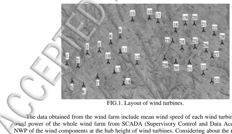
[image:2.595.67.451.499.721.2]In order to verify these three wind speed correction models and conduct wind power forecasting as well, a wind farm located at the northwest of China is taken as an example. The wind farm covers an area of about 17.5km2 and consists of 33×1.5MW wind turbines which have the hub height of 80m. The layout of wind turbines is shown in fig.1.
FIG.1. Layout of wind turbines.
B. Source of NWP data
The input NWP data used in this paper is the Weather Research and Forecasting (WRF)19 mesoscale wind, provided by the State Key Laboratory of Alternate Electrical Power System with Renewable Energy Sources.
The WRF model is initialized every day with the prediction of Global Forecasting System (GFS) released by National Centres for Environmental Prediction (NCEP). GFS is corresponding to the assimilation of atmospheric data at 00:00 GMT, and the forecast horizon is 72h ahead. The initial field20 of the NWP is from the NCEP Final (FNL) Operational Global Analysis data at 1°×1° resolution, which is prepared operationally every six hours. The FNLs are made with the same model as GFS, but the FNLs are prepared about an hour or so after the GFS is initialized. The FNLs are delayed so that more observational data can be used. The GFS is run earlier in support of time critical forecast needs, using the FNL from the previous six-hour cycle as part of its initialization.
The computation domain takes met mast location as the centre and has an extension of about 1800km over horizontal direction. Nested grid technique is adopted, and the initial field is downscaled to a resolution of 6km×6km by the WRF model.
C. Analysis of NWP wind speed estimates
Due to the coarse spatial resolution of the NWP data, it can only reflect the average wind within a certain area, and cannot represent for the wind speed and direction at single mast position accurately. If we take NWP data for the appropriate 6km×6km square to represent the data at the mast position as input to achieve wind power forecasting, this will result in significant error.
The two commonly used measures of error, Root Mean Square Error (RMSE) and Mean Absolute Error (MAE)21 are taken as the index of accuracy. The correlation coefficient (R) between NWP and measured wind speed is computed as well. These error measures and correlation coefficients are calculated according to equations (1), (2) and (3), where
u
i' andu
i respectively signify the NWPpredicted and measured wind speeds at time point
i
;n
is the number of forecasting samples.n u u RMSE n i i i
1 2 ' ) ( (1) n u u MAE n i i i
1 ' (2)
n 1 i 2 n 1 i i 2 i n 1 i 2 n 1 i ' i 2 ' i n 1 i n 1 i n 1 i i ' i i ' i ) u ( ) (u n ) u ( ) (u n u u u u nR (3)
Errors and correlation coefficients are calculated from
u
i' andu
i values over a year for the selected wind farm as shown in Table І. It can be seen that the NWP and measured wind speeds exhibit similar trends, i.e. are reasonably correlated as is intended. The errors however are large except autumn (September, October and November) and do not correlate so well with wind speed. December followed by February give the biggest errors, perhaps because they are months transitional between seasons.TABLE І. Comparison of NWP and measured wind speed over the sample year. Month
Mean value of WS (m/s)
Error of NWP WS
(m/s) Correlation
Coefficient
NWP Measured RMSE MAE
Jan 6.41 5.61 3.33 2.75 0.52
Feb 8.32 6.77 3.64 2.78 0.68
Mar 7.58 6.17 2.95 2.29 0.76
Apr 9.08 7.59 3.27 2.48 0.73
May 7.68 6.01 3.55 2.74 0.62
Jun 8.22 6.97 2.89 2.27 0.68
Aug 7.08 5.43 3.20 2.50 0.59
Sep 6.39 5.10 2.93 2.25 0.58
Oct 6.37 6.04 2.40 1.70 0.71
Nov 5.48 5.69 1.24 0.94 0.92
Dec 11.21 9.10 3.79 2.97 0.77
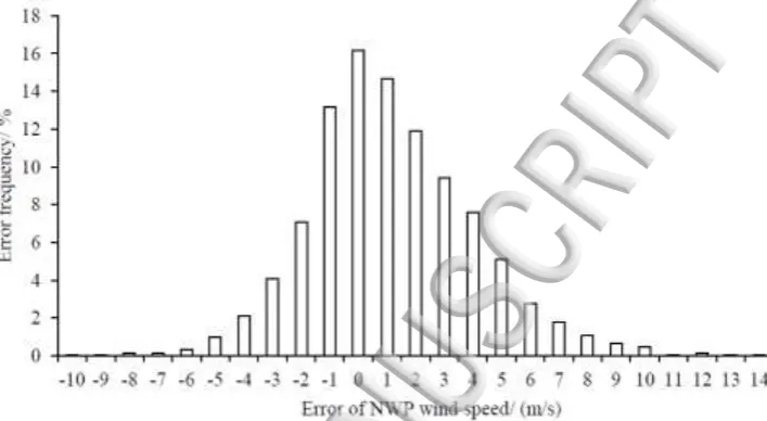
[image:4.595.121.475.210.404.2]The absolute error (AE) statistics for the NWP WS over the year can be binned into 1m/s intervals to provide a frequency distribution histogram, as illustrated in figure 2. The errors present skewed distribution with positive errors showing more frequent than negative ones, which means the NWP forecasts are generally higher than measurements.
FIG. 2. Frequency distribution for NWP wind speed error.
III. MODELLING PROCESS OF NWP WS CORRECTION AND WIND
POWER FORECASTING
Below rated power, the output power generation from a wind turbine follows roughly a cubic relationship with wind speed, and calculate results of WPF will amplify the errors in NWP wind speed. Therefore, it is particularly important to reduce any systematic errors in the NWP wind speed.
The key of correcting the NWP forecasts is to map the relationship between historical NWP and measured wind speed, and then to correct the wind speed estimates in accord with this relationship for future time steps. For the selected wind farm site, one year of NWP wind speed forecasts, measured wind speed and direction from met mast are available for use in the analysis. Data are divided into training and testing samples. For the training samples, the historical NWP wind speed and direction are taken as model input, and the measured wind speed at the corresponding time is taken as the learning targets. The test samples make use of the same variables. Three algorithms, MLR, RBF NN and Elman NN, are used to establish the NWP wind speed correction models.
A. Modelling of three WS correction models
In the process of forecast correction, linear regression, nonlinear RBF NN and Elman NN are used separately to build correction models. Both of the original forecasts and wind direction (expressed in terms of orthogonal components to avoid cyclic discontinuities) are taken as model inputs, and the corrected wind speed values are taken as the model output.
(1) Multiple Linear Regression
Multiple Linear Regression (MLR)22, 23 is a common method for establishing a relationship between inputs and outputs. The regression equation is applied for p forecasting input variables-
X
i (i=1, 2,…, p) and one forecasting object-Y
, and they all have the sample sizes of n.B
K
X
where, n y y y Y 2 1 , p 2 1 k k k K , n b b b B 2 1 , np n n p p x , x , x x , , x , x x , , x , x X 2 1 2 22 21 1 12 11 . Y X ) X X ( k k k K 1 p 2 1
(5)
Equation (5) is applied to calculate the estimated values
K
for the regression coefficientsK
, and these are used in the forecasting.(2) Radial Basis Function Neural Network
[image:5.595.159.430.313.514.2]A three-layer radial basis function neural network (RBF NN)24, 25 comprises an input layer, hidden layer and output layer. The structure is shown in Figure 3. A RBF NN represents hidden layer by a RBF. This method maps the input vectors into the hidden layer directly according to the cluster centre of the RBF, and there is no weight between input layer and hidden layer. Finally, the net output is gained by combining the outputs of hidden layer.
FIG. 3. Topology of RBF NN.
The mapping relationships within RBF network are made up of two parts. One is the nonlinear transformation from input space to hidden space, a clustering method is used to determine the node number of hidden layer, and the output of the j-th (j=1,2,..., m) hidden unit is
h
j(
x
)
. The other is the linear combination from hidden layer space to output layer space, denoted byf(
x
)
.]
σ
2
c
x
exp[
)
σ
,
c
x
(
)
x
(
h
2 j 2 j j j j
(6)j m
1 j
j
(
x
)
w
h
)
x
f(
(7))
(
is the transformation function in hidden unit,x
is a p-dimensional input vector,c
j andj
σ
are the center vectors and width of the j-th nonlinear transformation respectively;w
j is the connection weight between the j-th hidden unit and the output, calculated by least square method; m is the number of hidden units.(3) Elman Neural Network
connection layer records the output values of the hidden layer at previous time steps, and then returns these to the input of hidden layer. Via the delay and storage function of connection layer, the hidden layer can automatically connect its output to the input, which makes the net be more able to deal with dynamic information and can approach any nonlinear mapping with arbitrary precision.
FIG. 4. Topology of Elman NN.
Equation (8) is the expression of the nonlinear state-space of the Elman NN, where, t is the current time step,
y
is a one-dimensional output knot vector,x
is the p-dimensional input vector,u
is the r-dimensional unit vector of the hidden layer,u
c is a r-dimensional feedback state vector,w
1,w
2,w
3are the connection weight matrixes between different layers, b1 and b2 are the thresholds of input and hidden layer, g(*) is a linear transmission function of output layer, and f(*)is a non-linear arc tangent transmission function of hidden layer.
1) (t u (t) u )) b 1) (t x ( w (t) u f(w (t) u ) b (t) u g(w (t) y c 1 2 c 1 2 3 (8)
Elman NN adopts back propagation to modify the connection weights and thresholds, and the evaluation function is shown as equation (9), which is constructed by a sum of squares of errors. Where,
)
t
(
y
d is the target output in the time step of t.
T 1 t 2 d(t)] y [y(t)E - (9)
B. Modelling of CFD based wind power forecasting
To make full use of the NWP time series and limited measurement data, a CFD based physical wind power forecasting approach28 is used to assess the impact of improving the NWP wind speed forecasts on forecasting wind power. By establishing a flow character database, the physical WPF model puts the time-consuming flow field computation ahead of wind power forecasting process. For the wind farm under consideration, the detailed WPF procedures are explained below.
Firstly, the terrain elevation and roughness data for wind farm and surrounding area are obtained from a Geographic Information System, together with wind turbine locations. Secondly, considering of the aspect ratio and elevation drop of computing domain, the solution domain is specified as an extension of 7km out of the wind farm boundary in each horizontal direction and about five times the total elevation drop in height direction, and then an appropriate meshing is established. An RNG
conditions are distributed in 16 direction sectors evenly spaced from 0° to 337.5° with sector width of 22.5°. The combination of each wind speed and each wind direction comprises a discrete inflow condition, giving 192 discrete wind inflow conditions in total.
) ( 1 1 Z Z V V n
n (10) Based on the selected simulation scheme, commercial CFD software is used to calculate wind farm flow fields in the absence of wind turbines under 192 inflow conditions. All wind turbines in the wind farm are located according to their spatial coordinates. The Larsen wake model31 is employed to calculate wind speed wake deficits,
U
, displayed as equation (11), where,U
is the average wind speed at wind turbine hub height,A
is the swept area of rotor,C
T is the wind speed dependent thrust coefficient (taken from turbine manufacture’s data),c
is a dimensionless length,R
w is the radius of wake zone downwind whereL
x
.2 5 1 2 10 3 2 1 2 2 3 3 1 2
]
)
3
(
)
2
35
(
)
3
(
[
)
(
9
U
U
C
TAx
R
wc
C
TAx
c
(11)The wind speeds and directions at wind turbine hub height are calculated for each wind inflow condition, and then output power for those wind conditions is calculated according to wind turbine power curve. Finally, a database is established, comprising the wind inflow conditions, forecasting wind speed wind direction at hub height and output power for all wind turbines under each inflow condition.
The mesoscale NWP wind speed and wind direction is taken as inputs, searching for similar wind inflow conditions in the established database. Then interpolation methods are used to compute the output power of every wind turbine under given input conditions, corresponding to the forecast power for every single wind turbine in operation; eventually we get the predicted wind power for the whole wind farm in corresponding time.
IV. CASE STUDY
A. Evaluation of correction results
[image:7.595.62.463.572.738.2]Calculations using MLR, RBF NN and Elman NN algorithms are undertaken to correct the original NWP forecasts. The ratio between training and testing samples could be different under various wind farms, especially for complex terrain, the correction results will be sensitive to input wind conditions. Based on the experience32, 33 and simple sensitivity analysis against the proportion of training and testing samples, a ratio of 2:1 is selected in this case. The first twenty days in a month are taken as training samples to establish the three correction models, and the last ten days are taken as testing samples to validate the correction effects of each model. The time resolution of training data is 15min. The corrected wind speed values for the last ten days in a month represent the average correction to be applied to the whole month. For both training and testing data, there are three input variables (p=3) and only one output.
(1) Overall wind speed correction
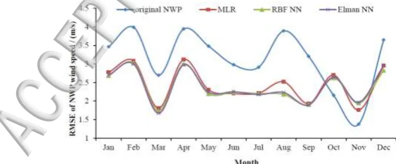
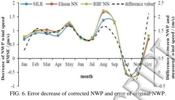
[image:8.595.143.451.134.310.2]The monthly RMSEs for the different wind speed corrections are calculated and plotted as shown in Fig 5. The monthly error reduction for the three correction methods are calculated and plotted in Fig.6 alongside the monthly average difference between original NWP and measured wind speed.
FIG. 6. Error decrease of corrected NWP and error of original NWP.
As can be seen in Figs. 5 and 6, the corrected wind speed from all three models have very similar RMSE, and they all maintain similar error variation trends to that of the original NWP. After correction, all the months show higher accuracy except for Oct. and Nov., the systematic errors of original NWP mode are also reduced dramatically. August shows the most obvious improvement, RBF NN, Elman NN, MLR model give a decrease of 1.71, 1.66 and 1.37 m/s respectively on the RMSE of original weather forecast. It can be seen from Fig. 6 that the error decrease provided by these three models have similar variation trends with the difference between the original and measured NWP WSs in every month. The original NWP have error peaks in Feb., Apr., Aug. and Dec., and so the correction effects for these months are superior to their adjacent months. The error drop of MLR is less than the other two models, so the correction effect of non-linear models is better than for linear models.
(2) Single point wind speed correction
(a) Original forecast (b) Corrected using MLR method
(c) Corrected using RBF NN method (d) Corrected using Elman NN method
[image:8.595.64.504.437.749.2]The absolute errors of each time point are calculated for the original and corrected NWP are averaged for wind speed intervals of 1m/s and the frequency distributions plotted as in Fig.7.
Figure 7 indicates that correction significantly improves accuracy and moreover the error range is reduced. For the three models the occurrence frequency for 0m/s to 1m/s has changed, rising from 30.3% to 32.2%, 32.9% and 33.0% comparing to the method. Compared with the other two models, Elman NN has a better single point correction effect, producing wind speed errors always less than 10m/s.
(3) Short-term wind speed correction
As can be seen from the above results, the correction methods’ performance depends on the time of year, but not in a systematic manner. May and August demonstrate good performance while October and November show error increases. Short-term variation trends (over a few days) for measured wind speed, original NWP and the corrected forecasts are compared for these four months, as shown as Fig. 8.
Fig. 8 shows that, as for the short-term correction, all these four corrected WS curves follow the same variation trends as the original NWP. Compared with the measured wind speed, the original forecasts have temporal and wind speed errors. For May and August the original forecasts are at times well in excess of the measured values, perhaps reflecting synoptic variations in weather, while for November the peaks in wind speed are captured well by the NWP. In Fig. 8(a) and Fig. 8(b), the corrected wind speeds minimize the peaks and narrow the gaps between the predicted and measured WS, which effectively reduce the systematic error of mesoscale NWP. In Fig. 8(c) and Fig. 8(d), the actual WS value is higher than the original NWP, and the relationship between them is not consistent with the trend of the whole year. Therefore, it is not recommended to carry on NWP corrections for October and November. Future research is required to assess whether it applies generally to other sites.
(a) May
(c) October
(d) November
FIG. 8. Short-term trends comparison for different wind speeds in four months. B. Analysis of WPF results
(1) WPF results under different input forecast wind speeds
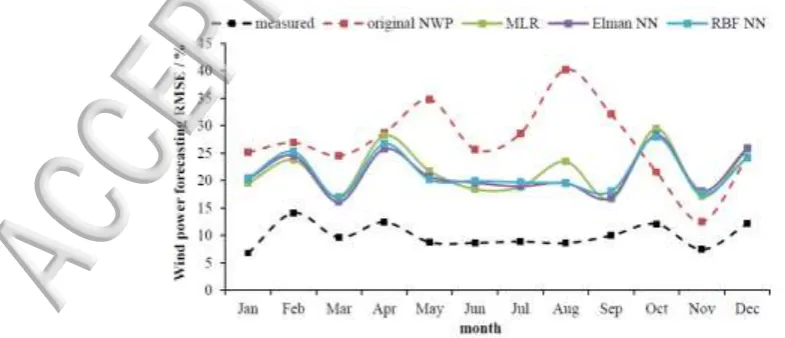
[image:10.595.61.454.574.743.2]In order to assess WPF errors for different inputs and analyze the impact of wind speed correction on WPF, the measured, original NWP and three corrected NWP WSs are respectively taken as the input of WPF model. The monthly RMSE of forecasting wind power is calculated and the error curves of different forecasting output power produced by the five inputs are presented in figure 9.
Fig. 9 illustrates that among the five approaches to forecasting wind power, the ones taking measured and original NWP WS as input generate the lowest and highest WPF error respectively, and the annual average RMSE are 10.04% and 27.78% respectively. Compared with taking the original NWP as input, the three corrected NWP separately lead to a drop of 5.58%, 6.13% and 6.18% on WPF RMSE. August has the most obvious forecasting improvement with RMSE decreases, which are 16.76%, 20.79%, 20.67% for the three correction models. In consequence, carrying out correction to the NWP WS will surely result in useful improvement of WPF accuracy.
In spring and winter, the three correction error curves are close to each other and the different correction models have little influence on the error of forecasting wind power, while in summer and autumn, the three correction WS error curves are distinct and different correction methods have great influence on resulting WPF error.
(2) Relationships between forecasting wind power and NWP wind speed
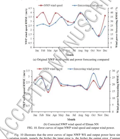
In contrast, it has been established above that the selection of correction model does not significantly affect the improvement of NWP wind speed forecasts, but the nonlinear models perform a little better than the linear one. The non-linear Elman NN model is taken as an example to analyse the relationship between input NWP WS and output forecasting wind power.
(a) Original NWP wind speed and power forecasting compared
[image:11.595.62.460.267.725.2](b) Corrected NWP wind speed of Elman NN
FIG. 10. Error curves of input NWP wind speed and output wind power.
mainly depend on the translation from wind speed to power. Thus, carrying on NWP WS correction will provide guidance for the separation of factors that influence WPF accuracy and lead to improvement of WPF model.
V. CONCLUSIONS
Mesoscale NWPs have a rough spatial resolution, which in turn restricts the precision of WPF based on such wind speed estimates. The MLR, RBF NN and Elman NN models are established to correct the NWP estimates of wind speed in this paper. The measured wind speed, the original NWP, and three corrected NWP forecasts are adopted to realize the CFD based wind power forecasts. Based on the case study presented, the following conclusions can be drawn:
(1) Compared with measurement data, the highest monthly RMSE of NWP WS is up to 3.64m/s. Its error distribution takes on seasonal characters, autumn has a lower prediction error than the other three seasons. For a single predicted time point, the probability of high errors exceeds that for low errors.
(2) Compared with the original NWP forecasts, the three correction methods significantly improved accuracy both over the whole year, and also over the short-term and for individual time steps. The correction effect of non-linear models is superior to linear ones. The highest RMSE drop for a single month, produced by RBF NN, can reach as high as 1.71m/s.
(3) All three correction methods decrease the temporal wind speed errors as well as the peak error values apparent in the original NWP estimates. The correction methods improve to a greater extent the forecasting wind power, more in summer and autumn than in spring and winter. The NWP wind speed forecasting performance in autumn is distinct from that of the rest of the year, so it is not recommended to carry on wind speed correction in this season. Future research is required to assess whether it applies generally to other sites.
(4) Errors in wind forecasts and forecast wind power follow similar annual trends, WPF precision increases when the precision of input wind speed increases. The three established correction models can improve the WPF accuracy by 5.58%, 6.13%, 6.18% respectively.
ACKNOWLEDGEMENTS
The work is supported by the National Natural Science Foundation of China (Grant No. 51376062, No.51206051) and the Fundamental Research Funds for the Central Universities (2015XS55).
REFERENCES
1
Xiaochen Wang, Peng Guo, Xiaobin Huang, “A review of wind power forecasting models,” Energy Procedia 12, 770-778 (2011).
2
Ma Lei, Luan Shiyan, Jiang Chuanwen, Liu Hongling, Zhang Yan, “A review on the forecasting of wind speed and generated power,” Renewable & Sustainable Energy Reviews 13, 915-920 (2009). 3
Ziqiao Liu, Wenzhong Gao, Yih-Huei Wan, et al., “Wind power plant prediction by using neural networks,” Energy Conversion Congress and Exposition, 3154-3160 (2012).
4
Kariniotakis G, Pinson P., “Evaluation of the MORE-CARE wind power prediction platform. Perfrmance of the fuzzy logic based models,” EWEC, 2003.
5
M.A. Mohandes, T.O. Halawani, S. Rehman, et al., “Support vector machines for wind speed prediction,” Renewable Energy 29, 939-947 (2004).
6
Landberg L, “Short-term prediction of local wind conditions,” Journal of Wind Engineering and Industrial Aerodynamics 89, 235-245 (2001).
7
Giebel G, Badger J, Perez I M, et al., “Short-term forecasting using advanced physical modelling-the results of the Anemos project,” Proceedings of the European Wind Energy Conference, 2006.
8
Efe B, Unal E, Mentes S, et al., “72hr forecast of wind power in Mani̇sa, Turkey by using the WRF model coupled to WindSim,” Renewable Energy Research and Applications, 1-6(2012).
9
Yongqian Liu, Jie Yan, Shuang Han, Infield David, De Tian, Linyue Gao, “An optimized short-term wind power interval prediction method considering NWP accuracy,” Chinese Science Bulletin 59, 1167-1175 (2014).
10
11
G. Galanis, P. Louka, P. Katsafados, et al, “Applications of Kalman filters based on non-linear functions to numerical weather predictions,” Annales Geophysicae. Copernicus GmbH 24, 2451-2460 (2006).
12
Danforth C M, Kalnay E, Miyoshi T, “Estimating and correcting global weather model error,” Monthly weather review 135, 281-299 (2007).
13
Gary M. Garter, J. Paul Dallavalle, Harry R. Glahn, “Statistical Forecasts Based on the National Meteorological Center’s Numerical Weather Prediction System,” Weather and Forecasting 4, 401-412 (1989).
14
Harry R. Glahn, Dale A. Lowry, “The use of model output statistics (MOS) in objective weather forecasting,” Journal of Applied Meteorology and Climatology 11, 1203-1211 (1972).
15
F. Anthony Eckel, Clifford F. Mass, “Aspects of effective mesoscale, short-term ensemble forecasting,” Weather and Forecasting 20, 328-350 (2005).
16
Delle Monache L, Nipen T, Liu Y, et al, “Kalman filter and analog schemes to postprocess numerical weather predictions,” Monthly Weather Review 139, 3554-3570 (2011).
17
Jakob Themeßl M, Gobiet A, Leuprecht A, “Empirical‐statistical downscaling and error correction of daily precipitation from regional climate models,” International Journal of Climatology 31, 1530-1544(2011).
18
Zjavka L, “Wind speed forecast correction models using polynomial neural networks,” Renewable Energy 83, 998-1006(2015).
19
Joseph B Klemp, “Weather research and forecasting model: A technical overview,” The 84th AMS Annual Meeting, Seattle, 10-15 (2004).
20
http://rda.ucar.edu/datasets/ds083.2/#!description 21
Li Li, Yimei Wang, Yongqian Liu, “Wind velocity prediction at wind turbine hub height based on CFD model,” International Conference on Materials for Renewable Energy and Environment, 411-414 (2013).
22
Huang Jiayou, “Meteorology statistical analysis and forecasting methods,” Beijing: China Meteorological Press (2010).
23
Zhang Xiunian, Cao Jie, Yang Suyu, Zha Minghui, “Multi-model compositive MOS method application of fine temperature forecast,” Journal of Yunnan University(Natural Science Edition) 33, 67-71 (2011).
24
Moody J, Darken C J, “Fast learning in networks of locally-tuned processing units,” Neural computation 1, 281-294 (1989).
25
I. R. H. Jackson, “Convergence properties of radial basis functions,” Constructive approximation 4, 243-264 (1988).
26
Jeffrey L. Elman, “Finding structure in time,” Cognitive science 14, 179-211 (1990). 27
Jujie Wang, Wenyu Zhang, Yaning Li, et al, “Forecasting wind speed using empirical mode decomposition and Elman neural network,” Applied Soft Computing 23, 452-459 (2014).
28
Li Li, Yongqian Liu, Yongping Yang, Shuang Han, Yimei Wang, “A physical approach of the short-term wind power prediction based on CFD pre-calculated flow fields,” Journal of Hydrodynamics 25, 56-61 (2013).
29
Yakhot V, Orszag S A, “Renormalization group analysis of turbulence. I. Basic theory,” Journal of Scientific Computing 1, 3-51 (1986).
30
Swinbank W C, “The exponential wind profile,” Quarterly Journal of the Royal Meteorological Society 90, 119-135 (1964).
31
Gunner C. Larsen, “A simple wake calculation procedure,” RISØ-M-2760, Risø National Lab, 19-25 (1988).
32
Santamaría-Bonfil G, Reyes-Ballesteros A, Gershenson C, “Wind speed forecasting for wind farms: A method based on support vector regression,” Renewable Energy 85, 790-809 (2016).
33
FIG. 2. Frequency distribution for NWP wind speed error. 0
2 4 6 8 10 12 14 16 18
-10 -9 -8 -7 -6 -5 -4 -3 -2 -1 0 1 2 3 4 5 6 7 8 9 10 11 12 13 14
E
rr
o
r
fr
eq
u
en
cy
/
%
FIG. 4. Topology of Elman NN.
Output layer
Hidden layer
Input layer b2
b1
Connection layer
u(t) y(t)
… x
p(t-1)
uc(t) w2
w3
w1
u1 ,u2 ,… ur u
c1 ,uc2 ,…ucr
FIG. 5. Annual RMSE variation of corrected and original NWP wind speed (based on last 10 days of
each month). 1
1.5 2 2.5 3 3.5 4 4.5
Jan Feb Mar Apr May Jun Jul Aug Sep Oct Nov Dec
RM
SE
o
f
NWP
w
ind
s
peed
/ (
m
/s
)
Month
FIG. 6. Error decrease of corrected NWP and error of original NWP. -0.5 0 0.5 1 1.5 2 2.5
-1 -0.5 0 0.5 1 1.5 2
Jan Feb Mar Apr May Jun Jul Aug Sep Oct Nov Dec
Dif
fer
ence
bet
w
ee
n
NWP
a
nd
m
ea
sured
w
ind
s
peed
/ (
m
/s
)
D
ec
re
a
se
o
f
NWP
w
ind
s
peed
RM
SE
/ (
m
/s
)
month
(a) Original forecast
FIG. 7. Error frequency distributions for different correction methods 0
5 10 15 20 25 30 35
0.5 1.5 2.5 3.5 4.5 5.5 6.5 7.5 8.5 9.5 10.5 11.5 12.5
E
rr
o
r
fre
qu
ency
/ %
(b) Corrected using MLR method
FIG. 7. Error frequency distributions for different correction methods 0
5 10 15 20 25 30 35
0.5 1.5 2.5 3.5 4.5 5.5 6.5 7.5 8.5 9.5 10.5
E
rr
o
r
fre
qu
ency
/ %
(c) Corrected using RBF NN method
FIG. 7. Error frequency distributions for different correction methods 0
5 10 15 20 25 30 35
0.5 1.5 2.5 3.5 4.5 5.5 6.5 7.5 8.5 9.5 10.5
E
rr
o
r
fre
qu
ency
/ %
(d) Corrected using Elman NN method
FIG. 7. Error frequency distributions for different correction methods 0
5 10 15 20 25 30 35
0.5 1.5 2.5 3.5 4.5 5.5 6.5 7.5 8.5 9.5
E
rr
o
r
fre
qu
ency
/ %
(a) May
FIG. 8. Short-term trends comparison for different wind speeds in four months. 0
2 4 6 8 10 12 14 16 18
5/21 0:00 5/23 0:00 5/25 0:00 5/27 0:00 5/29 0:00 5/31 0:00
Wi
n
d
s
p
eed
v
a
lu
e
/ (
m
/s
)
Time points
(b) August
FIG. 8. Short-term trends comparison for different wind speeds in four months. 0
2 4 6 8 10 12 14 16 18
8/21 0:00 8/23 0:00 8/25 0:00 8/27 0:00 8/29 0:00 8/31 0:00
Wind
s
peed
v
a
lue
/ (
m
/s
)
Time points
(c) October
FIG. 8. Short-term trends comparison for different wind speeds in four months. 0
2 4 6 8 10 12 14 16 18
10/21 0:00 10/23 0:00 10/25 0:00 10/27 0:00 10/29 0:00 10/31 0:00
Wind
s
peed
v
a
lue
/ (
m
/s
)
Time points
(d) November
FIG. 8. Short-term trends comparison for different wind speeds in four months. 0
2 4 6 8 10 12 14 16 18
11/21 0:00 11/23 0:00 11/25 0:00 11/27 0:00 11/29 0:00
Wind
s
peed
v
a
lue
/ (
m
/s
)
Time points
FIG. 9. Annual RMSE variation of forecasting wind power forecasts for different input wind speeds 0
5 10 15 20 25 30 35 40 45
Jan Feb Mar Apr May Jun Jul Aug Sep Oct Nov Dec
Wind
po
w
er
f
o
re
ca
st
ing
RM
SE
/ %
month
(a) Original NWP wind speed and power forecasting compared
FIG. 10. Error curves of input NWP wind speed and output wind power. 0 5 10 15 20 25 30 35 40 45
0 0.5 1 1.5 2 2.5 3 3.5 4 4.5
Jan Feb Mar Apr May Jun Jul Aug Sep Oct Nov Dec
Wind
po
w
er
f
o
re
ca
st
ing
RM
SE
/ %
NWP
w
ind
s
peed
RM
SE
/ (
m
/s
)
Month
(b) Corrected NWP wind speed of Elman NN
FIG. 10. Error curves of input NWP wind speed and output wind power. 0 5 10 15 20 25 30
0 0.5 1 1.5 2 2.5 3 3.5
Jan Feb Mar Apr May Jun Jul Aug Sep Oct Nov Dec
Wind
po
w
er
f
o
re
ca
st
ing
RM
SE
/ %
NWP
w
ind
s
peed
RM
SE
/ (
m
/s
)
Month