Wind power forecasts using Gaussian processes and numerical weather prediction

Wind Power Forecasts using Gaussian Processes

and Numerical Weather Prediction

Niya Chen, Zheng Qian, Ian T. Nabney, Xiaofeng Meng

Abstract—Since wind at the earth’s surface has an intrinsically complex and stochastic nature, accurate wind power forecasts are necessary for the safe and economic use of wind energy. In this paper, we investigated a combination of numeric and probabilistic models: a Gaussian Process (GP) combined with a Numerical Weather Prediction (NWP) model was applied to wind-power forecasting up to one day ahead. First, the wind-speed data from NWP was corrected by a GP, then, as there is always a defined limit on power generated in a wind turbine due to the turbine controlling strategy, wind power forecasts were realized by modeling the relationship between the corrected wind speed and power output using a Censored GP. To validate the proposed approach, three real-world datasets were used for model training and testing. The empirical results were compared with several classical wind forecast models, and based on the Mean Absolute Error (MAE), the proposed model provides around 4% to 11% improvement in forecasting accuracy compared to an Artificial Neural Network (ANN) model, and nearly 17% improvement on a third dataset which is from a newly-built wind farm for which there is a limited amount of training data.

Index Terms—Wind power forecasting, Gaussian Process, Nu-merical weather prediction, Censored data

I. INTRODUCTION

As a green and renewable energy resource, the utilization of wind energy has been growing rapidly around the world [1]. In China, the current total capacity of wind farms is approx-imately 75.6 GW, with a growth rate of 21.2% in 2012 [2]. However, the intrinsically variable and uncontrollable char-acteristics of wind pose several operational challenges. Thus wind power prediction is an essential process for the mainte-nance of wind power units and energy reserve scheduling [3], [4].

Accurate short-term wind power forecasts with a predic-tion horizon from one hour to several days are critical to optimise the scheduling of wind farm maintenance and re-serve electricity generation: these have an impact on grid reliability and market-based ancillary service costs. Broadly speaking, there are three approaches for short-term wind power forecasting: physical Numerical Weather Prediction (NWP) models, statistical models based purely on historical data, and statistical models with NWP data as additional exogenous inputs. Physical models have advantages over longer horizons (from several hours to dozens of hours), because they include (3D) spatial and temporal factors in a full fluid-dynamics model of the atmosphere. However, such models have limi-tations, such as the limited observation set for calibration (a

Ian T. Nabney is with the Non-linearity and Complexity Research Group, Aston University, Birmingham, UK e-mail: [email protected]

Niya Chen, Zheng Qian and Xiaofeng Meng are with Beihang University, Beijing, China.

serious issue given the extremely large number of variables in these models), the relatively limited spatial resolution possible over such a wide area (typically the whole earth), and the impossibility of accounting for local topography [5]. Statistical models which use only historical wind speed and power data and do not include any explicit model of the physical processes have been developed based on single models or hybrids of several methods, such as autoregressive integrated moving average (ARIMA) [6], [7], Kalman filters [8], artifi-cial neural networks [9], [10], support vector machines [11], [12] and Bayesian theory [13]. Since wind has an intrinsic non-stationary character, these purely statistical models are effective only for very short-term forecasts (about 1-4 hours ahead), and generally present very inaccurate predictions as the forecast horizon grows [14]. To overcome these limitations and obtain longer forecast horizons, some authors have combined both types of model, by using NWP (Numerical Weather Prediction) data from a physical model as inputs to a statistical model [15], [16].

Two forecasting systems based on artificial neural networks using NWP data and measured power generation from Super-visory Control And Data Acquisition (SCADA) systems as inputs for short-term wind power prediction (over a horizon of 72 hours) are presented in [17]: they can be used for electricity market bid offers and wind-farm maintenance tasks. The average RMS errors of the two presented forecast systems vary from 14% for the 12-24 hour horizon to 19.7% for the 48-72 hour horizon. Another forecast model combined with NWP data is proposed by Vaccaro [18], in which one-day-ahead wind power forecasting is based on information amalgamation from a local atmospheric model and measured data. De Giorgi [19] developed a series of forecast systems by combining Elman and MLP neural networks, and predicted power production of a wind farm with three wind turbines for 5 time horizons: 1, 3, 6, 12 and 24 hours. The normalized absolute average error of the presented systems vary from 5.67% to 15.50% depending on forecast time and different combinations of networks.

Recently, as an effective non-linear prediction method, Gaussian Processes (GP) have been applied in many domains, both in regression [20] and classification [21], including wind energy prediction. Jiang and Dong focused on very short term (<30min) wind-speed prediction using GPs [22]. They evaluated their model on real-world datasets, and found that the GP performs better than ARMA and the Mycielski algo-rithms [23].

In this paper, wind-farm datasets including NWP results and measured data from SCADA system are analyzed and applied

to wind power forecasting over a horizon of up to one day, using a Gaussian Process. The main innovations in this paper are:

1) The predicted wind speed from an NWP model is

corrected using a GP with predicted wind speed, wind

direction, temperature, humidity and pressure as inputs. The simplification of the regression task (by modeling a correction to the NWP data) helps to improve perfor-mance compared with earlier methods.

2) Automatic Relevance Determination (ARD) is used for feature selection in order to improve generalization performance.

3) A censored Gaussian Process (CGP) method is applied

to build the relationship between corrected wind speed and wind power, as wind power generation is censored due to the controlling strategy of the wind turbine. 4) A subset of high-wind speed data is treated separately,

because of its different characteristics as shown on analysis of the initial models.

5) Historical wind-speed data from a SCADA system is used as an additional input to the forecasting model for 1-4 hours-ahead prediction, since we have proved this to be effective in this range of time horizons.

6) The influence on forecast accuracy of training set history is investigated, and empirical results show that the GP method is able to obtain better prediction performance when there is limited data for model training than other techniques.

Section II describes the NWP model used to provide daily forecasts of meteorological variables. Section III defines the Gaussian Process, Automatic Relevance Determination (ARD) and censored GP methods applied to build all the regression models. Section IV describes the whole detailed modeling process from NWP data to forecast wind power results. Simulation results are presented and analyzed in Section V. Finally, Section VI includes the overall conclusions.

II. NWPMODEL

Numerical weather prediction uses hydrodynamic and ther-modynamic models of the atmosphere to predict weather based on certain initial-value and boundary conditions. Though there were attempts since the 1920s, reliable numerical weather prediction was not achieved until the development of powerful computers. Nowadays, a number of global and regional NWP forecast models have been developed. In our research, we use the WRF (Weather Research and Forecasting) NWP model. WRF was created through a partnership that includes NCAR (National Center for Atmospheric Research), NOAA (National Oceanic and Atmospheric Administration), and more than 150 other organizations and universities in the United States and internationally, and is released as a free model for public use [24].

In general, short-term wind-power forecasting needs pre-dictions from an NWP model with high spatial resolution. In our case, the WRF model with the Advanced Research WRF (ARW) core is used. First, the accurate geographical position and hub height of one wind turbine or wind mast in a wind

farm is chosen as a reference point, then a 3-layer nested grid is built centered around this point. Finally, using the initial data provided by Global Forecast System (GFS) model, the NWP data can be abstracted from the corresponding point in the 3rd layer. The NWP data used in our paper is available at 20:00 GMT every day. The data including wind speed and direction, temperature, humidity and pressure, is provided at an interval of 10 minutes for the following 72 hours.

The Chinese government imposes very specific demands on wind-power forecasting in the energy sector, which include the following conditions: the forecast error of 1-4 hour ahead should be less than 10% of wind turbine’s installed capacity; the 5-24 hour-ahead forecasting error should be below 20% of installed capacity. All the forecast errors contained in this paper are calculated using hourly data. Therefore, we focus on forecasting for a horizon from 1 to 24 hours for wind power, based on hourly sampled NWP data.

III. GAUSSIANPROCESSMETHODS

Recently, there has been much activity concerning the application of Gaussian process to machine learning tasks. Because a systematic and detailed explanation of Gaussian process regression and Automatic Relevance Determination (ARD) can be found in Rasmussen’s book [25], and the model

of censored GP was proposed by Groot [26], here we only

provide a brief description of these methods. A. Standard Gaussian Process

A Gaussian process f(x) can be completely specified by its mean function and covariance function, written as f(x) ∼ GP(m(x), k(x, x0)), where the mean functionm(x)

and covariance functionk(x, x0)are defined as m(x) =E[f(x)]

k(x, x0) =E[(f(x)−m(x))(f(x0)−m(x0))]. (1) Usually, the mean function is assumed to be zero and the target variable is normalised to have zero mean.

Consider the GP in a classic regression problem: assume we have a training setDofnobservations,D={(xi, yi)|i=

1, ..., n}, where x denotes an input vector of dimension D andy denotes a scalar output. As we have ncases ofx, the whole input data is represented by a D×nmatrix, and with targets collected in a vector y, we can write D = (X, y). Therefore, the key point of the regression problem is to model the relationship between inputs and targets, that is to build a function to satisfy,

yi=f(xi) +i, (2)

where the observed values y differ from the function values f(x)by additive noise, which is assumed to be an indepen-dent, identically distributed Gaussian distribution with zero mean and variance σ2

n, i.e. ∼ N(0, σ2n). Note that y is a linear combination of Gaussian variables and hence is itself Gaussian [27]. The prior ony becomes

E[y] =E[f+] = 0

whereKis a matrix with elementsKij =k(xi, xj), which is also known as the kernel function.

Given a training set D = (X, y), our goal is to make predictions of the target variablef∗ for a new inputx∗. Since we already have p(y|X, k) =N(0, K+σ2

nI), the distribution with new input can be written as

y f∗ ∼ N 0, K(X, X) +σ2 nI k(X, x∗) k(x∗, X) k(x∗, x∗) , (4) where k(X, x∗) = k(x∗, X)T = [k(x1, x∗), ..., k(xn, x∗)], which we will abbreviate as k∗. Then according to the prin-ciple of joint Gaussian distributions, the prediction result for the target is given by

¯ f∗=kT∗(K+σ2nI) −1_y V[f∗] =k(x∗, x∗)−k∗T(K+σ2nI)− 1_k ∗. (5) Now, the whole regression model based on Gaussian process is completed.

B. Automatic Relevance Determination

In practice, rather than fixing the covariance function for a Gaussian process model, we may prefer to use a parametric function and infer the parameter values from the observed data. This learning process, which is usually called ‘learning the hyperparameters’, can be accomplished by maximizing the log likelihood function lnp(y|θ) =−1 2ln|K| − 1 2y T_K−1_y−n 2 ln(2π). (6)

This function is maximized using a standard non-linear gradient-based optimization algorithm. A detailed description can be found in [25].

As the maximum likelihood can be used to determine the parameter values in the Gaussian process, we can extend this technique by incorporating a separate lengthscale parameter for each input variable, and hence the relative importance of different inputs can be inferred from the observed data, which is known as Automatic Relevance Determination. For example, the covariance function used in our model is the rational quadratic k(x, x0) =θ0 1 + D X i=1 li(xi−x0i) 2 !−v +b, (7) where b represents a bias, and all the hyperparameters can be contained in a vector θ = (θ0, L, b)T, where L denotes

the vector of all the lengthscale parameters L={l1, ..., lD}. The hyperparameters{l1, ..., lD}are used to implement ARD: as li becomes larger, the function becomes relatively more sensitive to the corresponding input variable xi. Therefore, the importance of each input variable is revealed, and inputs with a small value of li can be discarded.

C. Censored Gaussian Process

As a result of the wind-turbine control strategy, there is always a defined upper limit to the power generation of each turbine type. Denote the upper limit of power generation by C, the unrestricted power output by y∗ _{(a latent variable}

since it is not observed directly), and the observed output of wind turbine as y, then with the physical non-negative property of power also considered, we have

y=    0 if y∗≤0 y∗ if 0< y∗< C C if y∗≥C. (8)

In statistical terminology, the true values are ‘censored’ in that they are not observed directly but instead a different value is substituted. Exploratory analysis of the data shows that 1.1% percent of the data is approximately (within 1% of) the upper limit C and a further 5.4% percent is within 5% of the upper limit (and is thus in the range where the noise distribution of the unrestricted prediction overlaps significantly with the censored range). Thus it is important to account for this constraint in the model itself rather than simply pre-process the predictions of a ‘standard’ regression model by thresholding them atC.

Following Groot’s paper [26], we assume that the latent values y∗ = f(x) can be realized by a Gaussian process regression model, and use φ(.), Φ(.) to denote the standard normal density and cdf respectively, then the likelihood can be expressed as a mixture of Gaussian and probit likelihood terms L= n Y i=1 p(yi|fi) = Y yi=0 1−Φ _f i σ Y 0<yi<C ₁ σφ _y i−fi σ Y yi=C Φ _f i−C σ . (9)

By Bayes’ theorem, the posterior distribution over the latent variables is the product of the prior and the likelihood

p(f|X, y) = 1 Zp(f|X) n Y i=1 p(yi|fi), (10)

whereZ =p(y|X)is a normalization term called the marginal likelihood. However, this posterior is analytically intractable because of the form of the likelihood in equation (9): thus one has to use approximate techniques for computing it. Here we use an Expectation Propagation (EP) method: assume that the likelihood of latent variablefi isp(yi|fi)'ti(fi|Zei,eµi,σe

2

i), and abbreviate it asti. Then the posterior p(f|D)is approxi-mated byq(f|D)where q(f|D) = 1 ZEP p(f) n Y i=1 ti(fi|Zei,µ_ei,_eσi2) = 1 ZEP p(f)N(_eµ,Σ)e n Y i=1 e Zi, (11)

where ZEP is the normalization term. Then we update the ti approximations sequentially by the EP algorithm, finally the approximation to the posterior is computed, and the predictive distribution q(f∗) of input x∗ can be written as

q(f∗) =N(µ∗, σ2∗), where µ∗=k∗T(K+Σ)e −1_eµ

σ_∗2=k(x∗, x∗)−kT∗(K+Σ)e −1k∗,

(12) where k∗ = [k(x1, x∗), ..., k(xn, x∗)], as defined in Sec-tion III-A.

IV. MODELINGPROCESS

The forecasting framework proposed in this paper uses GP models and three additional features: 1. ARD is used to select model inputs; 2. predicted wind speed from the NWP model is corrected before modelling the mapping from wind speed to wind power; 3. detailed adjustments were applied to improve forecast accuracy, such as including historical data and building a separate model for high wind speed.

The NWP data usually includes several kinds of meteoro-logical information: wind speed, wind direction, temperature, air pressure, and humidity. It is clear that wind power mainly depends on the actual wind speed, however, we don’t know for sure if any other variable plays an important role too. The ARD toolbox in Netlab [28] was used to determine the appropriate inputs for each model mentioned in this paper.

Since wind power generation is mainly determined by wind speed, the most important practical task for companies operat-ing wind farms is to get accurate wind speed prediction. There are two ways to obtain wind power from NWP data: directly learning the model between NWP data and wind power using a censored GP; or correcting the error in NWP wind speed prediction first and then using this corrected wind speed to replace original NWP speed for forecasting power generation. The second method is based on the belief, underpinned by a large body of empirical analysis, that there are some systematic and stochastic biases present in the original NWP speed forecasts – the detailed empirical analysis is illustrated in Section V-B. We denote the first way of modeling wind power as GP-Direct, and the second as GP-CSpeed (meaning based on corrected speed).

A schematic of the whole modeling process of the proposed GP-CSpeed model, including ARD inputs selection and NWP speed correction, is shown in Figure 1. Firstly, an ARD model (ARD I) is applied to determine which features in NWP are most relevant to predict measured wind speed, then the corrected wind speed is obtained using a GP model with the selected inputs. Second, the wind speed in NWP data is replaced with the corrected speed from the first step, and another ARD model (ARD II) is used to choose features that are relevant to power generation. Finally, with the data of selected features used as inputs, a censored GP-based model is built for forecasting wind power.

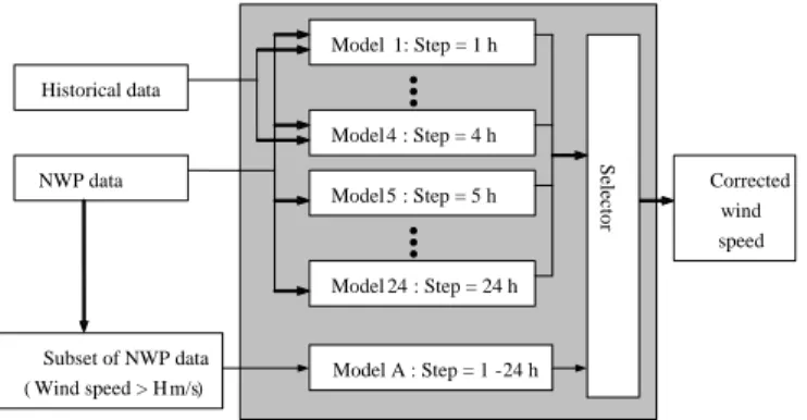
Figure 2 shows the detailed structure of the proposed correction process, which obtains corrected wind speed from selected NWP variables as shown in the dashed line box in Figure 1. Certain constraints are used to improve the accuracy of modeling. Since the character of wind changes with the diurnal cycle, the prediction error of the NWP model shows different properties depending on the forecast horizon (1–24 hours). Therefore, we built a separate model for each of the 24

Ⅰ

Ⅱ

Fig. 1. Modeling process of the proposed GP-CSpeed model.

hourly forecast horizons and the training dataset was divided into 24 subsets. Secondly, as mentioned before, historical data of measured wind speed turns out to be useful for very short-term forecasting, 1–4 hours ahead for our datasets according to empirical analysis (refer to SectionV-B), and is therefore included as an input for models 1–4 only (i.e. 1–4 hours forecast horizon). Thirdly, the prediction error of the NWP model is larger and more related to humidity when the predicted wind speed is high, thus we developed a separate GP model (labeled Model A in the figure) specifically to improve the correction accuracy when the predicted wind speed is larger than H m/s, where H denotes the threshold value of high speed and depends on the location of the wind farm.

NWP data Historical data Model 1: Step = 1 h Model 4 : Step = 4 h Subset of NWP data ( Wind speed > H m/s) Corrected wind speed Model 5 : Step = 5 h Model 24 : Step = 24 h Selector Model A : Step = 1 -24 h

Fig. 2. Structure of correction process.

As shown in Figure 2, models 1–24 give results of correc-tion for 1–24 hours-ahead predicted wind speed, while model A gives corrected wind speed for high speeds. The reason for just building one model for high wind speed, is that such data only accounts for about 5% of the whole dataset, and thus there is not enough data for training several high-speed models separately. The ‘selector’ component means that when the original predicted wind speed in the NWP data is larger thanH m/s, then the corresponding corrected wind speed in the result of model 1–24 is replaced by the output of model A.

V. EXPERIMENTALVALIDATION

Three real-world datasets based on wind farms were used in this paper to evaluate our approach. The first one is from a wind farm in Gansu province (denoted as Farm-G), which is located in the windy western part of China. The second,

denoted by Farm-J, is from Jiangsu province, a coastal area located in southern China. These two farms are about 2400km apart, and therefore the weather conditions are independent from each other. The third one is a recently built wind farm nearby Farm-J, denoted by Farm-R.

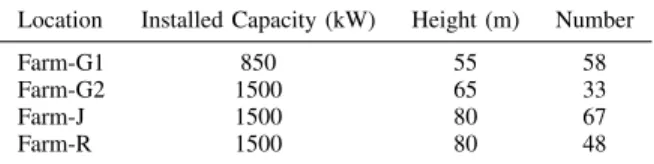
TABLE I WIND TURBINE PROPERTIES.

Location Installed Capacity (kW) Height (m) Number

Farm-G1 850 55 58

Farm-G2 1500 65 33

Farm-J 1500 80 67

Farm-R 1500 80 48

As shown in Table I, Farm-G is a large wind farm with 91 wind turbines, which are divided into two groups: the installed capacity of one kind is 850kW, and the other is 1500kW. Actually, the NWP data of Farm-G were obtained from two different models separately developed for these two groups, because of the difference in turbine height. Correspondingly, all the prediction models established in this paper are devel-oped separately for different wind turbine groups. Datasets from Farm-G and Farm-J have a time scale from April 2010 to April 2013: we have used a whole year from April 1st 2010 to April 1st 2011 as a training set, and the remainder as a test set. The newly built Farm-R only has 2 and a half months’ data, and is specially modeled in subsection V-D, to illustrate the performance of the proposed GP-CSpeed model on a small dataset.

A. Forecasting accuracy evaluation

Several criteria were used to evaluate the accuracy of the proposed approach. This accuracy is computed as a function of the measured wind speed or power. Four error measures were employed for model evaluation and model comparison: the Root Mean Square Error (RMSE), the Normalized Root Mean Square Error (NRMSE), the Mean Absolute Error (MAE),and Normalized Mean Absolute Percentage Error (NMAPE). The error measures are defined as follows

et=yt− ∧ y_t (13) RM SE= v u u t 1 n n X i=1 e2 i (14) N RM SE = v u u t 1 n n X i=1 e2 i × 100 C (15) M AE = 1 n n X i=1 |ei| (16) N M AP E= 1 n n X i=1 ei C×100 (17)

where yt represents the actual observation value at time t,

ˆ

yt represents the forecast value for the same period,nis the number of forecasts, and the installed capacity of wind turbine is denoted byC.

The NMAPE is used for wind power as a requirement of the Chinese government, and it is also a suitable expression to interpret the quality of forecast, since without normalization, the same value of |e| may imply very different performance according to different type of wind turbines with variant installed capacity.

As specified requirements are made separately for 1-4 hours (N M AP E≤10%) and 5-24 hours (N M AP E≤20%) fore-cast, we define an extra criterion to determine the prediction performance

Px=

1

m|{|ei| ≤x·C}| ×100%, (18) where m denotes the size of the corresponding test dataset, andx denotes the threshold NMAPE value, i.e. x= 0.1 for 1–4 hours forecast and x= 0.2 for 5–24 hours forecast. In this way the percentage of points which meet the requirements can be calculated.

B. Effectiveness of proposed model

First of all, ARD was applied to determine which NWP variables should be included as inputs to the speed correction model. Using the difference between measured wind speed and NWP predicted speed as the target variable, the relevance values are listed in Table II.

TABLE II

ARDRESULTS ON TWO FARMS.

Location Wind speed Wind di-rection Temperature Air pressure Humidity Farm-G1 1.5696 0.0002 3.4872 9.6381 2.5239 Farm-G2 0.3882 0.0463 2.2647 3.5917 0.9233 Farm-J 0.1203 0.0014 3.2269 0.0383 0.3569

We note that wind speed, temperature and humidity impact the prediction accuracy of 3 groups of wind turbines in 2 wind farms. For Farm-G, air pressure plays a much more im-portant role, which is reasonable considering its high altitude. Therefore, we choose these three features as inputs to the GP correction process for J, and add air pressure for Farm-G. By the same selection process, ARD is applied to choose features that are relevant to wind power: corrected speed and humidity for Farm-G, corrected speed and wind direction for Farm-J.

In order to illustrate the effectiveness of the whole modeling process, we show the detailed results for a single wind turbine from Farm-J. A comparison of the original NWP wind speed error and the results of two correction models (both with and without historical data) is displayed in Figure 3. It can be clearly observed that both corrected results are much better than the original NWP data, and for the short-horizon forecasts, the addition of historical data successfully reduced prediction error, but introduced a small amount of additional error (probably due to overfitting) as the forecast horizon grows. Therefore, we chose to add historical data for 1–4 hours ahead wind speed correction only.

In order to display and analyze the performance of the cor-rection models, we first divided the dataset by NWP-predicted

0 2 4 6 8 10 12 14 16 18 20 0 2 4 6 8 10 12 14 NWP speed m/s RMSE m/s NWP speed error Corrected error (a) 13 14 15 16 17 18 19 1 2 3 4 5 6 7 8 NWP speed m/s RMSE m/s NWP speed error Corrected error Corrected error by Model A

(b)

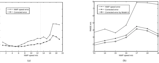
Fig. 4. Influence of building additional model for high speed NWP data. (a) Standard correction model. (b) Comparison with additional high-speed model.

0 5 10 15 20 25 1 1.2 1.4 1.6 1.8 2 2.2 2.4 2.6

Forecast step / hour

RMSE m/s

NWP speed error Corrected error

Corrected error (historical data added)

Fig. 3. Comparison of forecast error of 3 models.

wind speedyˆt, that isDs={s−1≤yˆt< s, s= 1,2, ...}, then calculated the RMSE of each subsetDs, and plotted the RMSE value against s. As shown in Figure 4(a), the performance of the correction models 1–24 is consistently good whens≤10: however, for higher wind speed the corrected results become worse. On further analysis, it was noticed that humidity is influential as wind speed increases, especially for s >13, as shown by Table III (compare with Table II).

TABLE III

ARDRESULTS ON HIGH-SPEED SUBSET.

Location Wind speed Wind di-rection Temperature Air pressure Humidity Farm-G2 3.3159 0.0002 18.183 12.436 26.099

As a result, the high-speed subset is selected with a thresh-old H = 13 m/s for Farm-J, and special correction model A can be built with predicted wind speed, temperature and humidity as inputs. By the same analysis process, the threshold value is determined to be H = 12 m/s for Farm-G1, and

H = 13m/s for Farm-G2. The correction results for the high-speed subset are shown in Figure 4(b), which illustrates the effectiveness of building model A for high speed data.

With the whole correction process, the corrected wind speed has a much better test-set accuracy than the original NWP wind-speed predictions, as shown in Table IV.

TABLE IV

SPEED FORECAST ERROR OF A TURBINE INFARM-J.

MAE Data RMSE(m/s) MAE(m/s) Improvement NWP-speed 2.4160 1.8663 -Corrected speed 1.6405 1.2399 33.56%

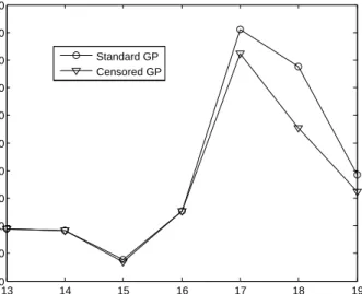
Since the generated wind power is limited to the installed capacityCof a wind turbine by a controller, a censored GP is used in this paper to build the wind power forecasting model. The RMSE of predicted wind power from both censored and standard GP models is calculated and the predictions with a high corrected wind speed s is plotted in Figure 5, because this is where the generated wind power might be censored. The standard GP results include a threshold on the GP output at capacity, but the GP can predict impossible values, whereas the censored GP builds the constraint into the parameter learning process. From the figure, we can clearly see that the censored and standard GPs perform equally well at medium speed, but as the wind speed grows, the difference becomes more obvious and the censored GP is more accurate. The improvement in accuracy at very high predicted wind speeds is because at those speeds (provided the speed prediction is reasonably accurate), the turbine output is alwaysCand hence is easier to predict. C. Comparative results

In this section we present the results of our power-prediction framework and some benchmarks: the persistence model, ARIMA method, and a multi-layer perceptron (MLP) neural network. The persistence method simply uses the current value as the forecast, which means that at time t, the prediction

ˆ

13 14 15 16 17 18 19 300 350 400 450 500 550 600 650 700 750 800

Corrected wind speed m/s

RMSE of power kW

Standard GP Censored GP

Fig. 5. Power prediction accuracy for normal and censored GP.

power data may be invalid because of a turbine fault (invalid data was excluded from the dataset at the pre-processing stage), we use the current wind speed data in this model, and calculate the wind power with the wind turbine curve. The ARIMA method is a classical time series based model that has been frequently applied to wind forecasting [7], and is therefore picked as a benchmark.

MLP networks have been applied to short-term wind power forecasting before, and have achieved a much better perfor-mance than the persistence method [29], hence an MLP-based model (MLP-CSpeed) which builds a relationship between selected NWP features (using ARD) and wind power is chosen for comparison. A 9-neuron hidden layer was chosen for the MLP model, based on empirical cross-validation results (model comparison on a validation set).

0 5 10 15 20 25 0 200 400 600 800 1000 1200 1400 1600

Forecast step / hour

Wind power / kW

Measured power GP−CSpeed MLP−CSpeed

Fig. 6. One-day-ahead wind power forecasting.

An example of one-day-ahead wind power forecasting for one wind turbine is illustrated in Figure 6. The forecast error is reasonably small for very-short term forecasting (1– 4 hours ahead). The figure clearly shows how the forecast

error increases with the forecast horizon, but the proposed GP-CSpeed model still captures the shape of the actual power time series, and has better performance than the ML model.

Our empirical results show that one well-trained forecast model is also suitable for other turbines of the same type located at the same wind farm: this represents a considerable time saving in model development. The results of applying the proposed model to the test datasets are shown in Tables V–VII.

TABLE V

POWER FORECAST ERROR OFFARM-G1 (NOMINAL POWER: 49.3MW).

Model RMSE (MW) NRMSE MAE (MW) NMAPE Improve-ment1 P0_1-4h.1 P0_5-24h.2 Persistence 10.79 21.89% 7.49 15.19% - 55.91% 69.56% ARIMA 10.70 21.71% 7.40 15.00% 1.22% 58.64% 68.89% MLP 9.63 19.53% 7.04 14.28% 6.03% 37.27% 78.34% GP-Direct % % 65.91% 78.72% GP-CSpeed 8.74 17.72% 6.32 12.82% 15.64% 65.91% 81.49% 1. Improvement is calculated relative to the persistence method.

TABLE VI

POWER FORECAST ERROR OFFARM-G2 (NOMINAL POWER: 49.5MW).

Model RMSE (kW) NRMSE MAE (kW) NMAPE Improve-ment2 P0.1 1-4h P0.2 5-24h Persistence 10.69 21.60% 7.69 15.52% - 61.99% 70.01% ARIMA 10.50 21.21% 7.49 15.13% 2.51% 62.38% 70.82% MLP 8.76 17.70% 6.86 13.86% 10.72% 37.09% 75.58% GP-Direct % % 43.05% 77.85% GP-CSpeed 8.55 17.28% 6.12 12.36% 20.37% 66.89% 74.55% 2. Same as 1. TABLE VII

POWER FORECAST ERROR OFFARM-J (NOMINAL POWER: 100.5MW).

Model RMSE (kW) NRMSE MAE (kW) NMAPE Improve-ment3 P0_1-4h.1 P0_5-24h.2 Persistence 27.01 26.87% 18.53 18.43% - 59.43% 62.67% ARIMA 26.78 26.65% 18.13 18.03% 2.18% 60.89% 63.05% MLP 17.16 17.07% 11.70 11.64% 36.85% 53.91% 78.08% GP-Direct 17.16 17.07% 11.76 11.71% 36.48% 56.03% 78.62% GP-CSpeed 15.42 15.34% 10.34 10.29% 44.21% 62.50% 78.82% 3. Same as 1.

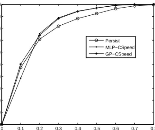
The results of wind power forecasting are shown in Ta-bles V–VII: we can analyze the performance more deeply by plotting the error distribution as in Figure 7. It is clearly shown that the proposed GP-CSpeed model presents the best performance in 1–4 hour forecast horizons, and a less obvious but still visible improvement in 5–24 hour horizons with a larger percentage of points having NMAPE less than 10%.

As we can see from Tables V–VII, the proposed GP-CSpeed model has better performance than the other models. In terms of MAE, the improvement of accuracy is 15.64%, 20.37% and 44.21% for 3 datasets. If comparing to MLP-CSpeed model, the improvement is 10.22% for dataset of Farm-G1, 10.79% for Farm-G2, and 11.66% for Farm-J.

All the models were run on a single computer (Intel Core 2 Duo CPU, 2.93 GHz, 2 GB memory): the mean computational cost for each model is listed in Table VIII.

0 0.1 0.2 0.3 0.4 0.5 0.6 0.7 0.8 0 10 20 30 40 50 60 70 80 90 100 Error threshold x

Percentage of points meet Px

Persist MLP−CSpeed GP−CSpeed

(a) 1–4 h forecast results

0 0.1 0.2 0.3 0.4 0.5 0.6 0.7 0.8 0 10 20 30 40 50 60 70 80 90 100 Error threshold x

Percentage of points meet Px

Persist MLP−CSpeed GP−CSpeed

(b) 5–24 h forecast results

Fig. 7. Error distribution of Farm-G2.

TABLE VIII

AVERAGE COMPUTATIONAL COST.

Model MLP-CSpeed GP-Direct GP-CSpeed Time 13.27s 83.64s 83.17s

D. Effectiveness of proposed model for small dataset Since wind power is seen as one of the most important carbon-free energy generation methods, many new wind farms are being built [2]. During their initial operation it is hard to obtain a significant quantity of historical data to build accurate forecasting models. In this section, we investigate the effectiveness of our GP method when there is little data. First of all, to analyze the influence of training set size, based on Farm-G2 dataset, various forecast results are obtained by changing the length of the training set, while test set is still 1 year long (from April 1st 2011 to April 1st 2012). The forecasting accuracy of proposed GP-CSpeed model is compared to MLP-CSpeed model in Figure 8.

0 200 400 600 800 1000 1200 1400 1600 1800 2000 2200 200 300 400 500 600 700 800 900

Number of training set /point

RMSE of power forecast /kW

GP−CSpeed MLP−CSpeed

Fig. 8. Forecasting accuracy influenced by length of training set.

As shown in Figure 8, the prediction error of the GP-CSpeed

model is already quite low when there is only one month of training set data. In addition, as the training set grows, the GP-CSpeed model achieves a stable high performance quickly, while the accuracy of the MLP-CSpeed model is still relatively poor.

Then, to validate the performance of the proposed model in a real-world application, a dataset from a newly built wind farm was used to build a forecast model and obtain prediction results. The newly built wind farm we focus on is located in the coastal area of China where wind energy is abundant, and there are plans to construct more wind farms in the region in the near future. The data, including 2 and a half months’ NWP and SCADA data, is divided into a 45-day training set and a 1-month test set. Note that one advantage of splitting the power prediction problem into separate wind-forecasting and power-prediction tasks is that the model mapping wind speed to power output can be reused on new wind farms provided the turbine is of a known type. The forecasting results are contained in Table IX.

TABLE IX

WIND POWER FORECAST ERROR, FARM-R 1500KWTURBINE.

Model RMSE (kW) NRMSE MAE (kW) NMAPE Improve-ment4 P0_1-4h.1 P0_5-24h.2 Persistence 447.74 0.2889 319.79 21.32% – 56.15% 56.50% MLP-CSpeed 381.61 0.2462 272.19 18.14% 14.88% 36.88% 64.47% GP-CSpeed 321.31 0.2073 225.04 15.00% 29.63% 47.84% 75.94% 4. Same as 1.

As shown in Table IX, despite of the limited quantity of data, the proposed GP-CSpeed model still performs an accept-able accuracy of forecast. This advantage is especially obvi-ous compared with the MLP-CSpeed model with a 17.32% improvement.

VI. CONCLUSION

Short-term wind power forecasting, which strongly impacts the safety and economics of the electricity grid, is an im-portant and challenging task, considering the uncontrollable and stochastic nature of wind. Current research in this domain

based on statistical models can be divided into two parts: fore-casts several hours ahead using only historical data; predictions dozens of hours ahead based on NWP data.

In this paper, we investigated a combination of numeric and probabilistic models: a Gaussian Process (GP) combined with a Numerical Weather Prediction (NWP) model was applied to one-day-ahead wind power forecasting. Certain methods were employed to improve the forecast accuracy: predicted wind speed is firstly corrected by GP before it is used to forecast wind power; as there is a defined limit on power generation of wind turbine, a censored GP is applied to build speed-power model; ARD is used to choose effective NWP variables as inputs of each model; for 1–4 hour ahead forecasts, historical data is added into modeling process; and a high wind-speed subset is treated separately by building a single forecast model. The simulation results shows that, compared to an MLP-CSpeed model, the proposed model has around 10% to 12% improvement of accuracy for the regular large datasets of Farm-G and Farm-J, and hence the effectiveness and perfor-mance of the GP-CSpeed model is proved. Furthermore, the proposed GP-CSpeed model is especially effective when there is limited training data, as it achieves an significant 17.32% improvement for dataset from newly built Farm-R.

ACKNOWLEDGMENTS

We are thankful to the National Fund for Creative Groups of China (Grant No. 61121003), for their support of the present study. This work has been partially supported by a BUAA Scholarship, which funded N.C.’s visit to Aston University. We are grateful for the comments of the anonymous reviewers which have materially improved this paper.

REFERENCES

[1] J. K. Kaldellis and D. Zafirakis, “The wind energy evolution: A short review of a long history,” Renewable Energy, vol. 36, no. 7, pp. 1887 – 1901, 2011. [Online]. Available: http://www.sciencedirect.com/science/article/pii/S0960148111000085 [2] G. W. E. Council, “Global wind statistics 2012,”Global Wind Report,

pp. 1–4, 2012.

[3] A. Costa, A. Crespo, J. Navarro, G. Lizcano, H. Madsen, and E. Feitosa, “A review on the young history of the wind power short-term prediction,” Renewable and Sustainable Energy Reviews, vol. 12, no. 6, pp. 1725 – 1744, 2008. [Online]. Available: http://www.sciencedirect.com/science/article/pii/S1364032107000354 [4] M. Lei, L. Shiyan, J. Chuanwen, L. Hongling, and

Z. Yan, “A review on the forecasting of wind speed and generated power,” Renewable and Sustainable Energy Reviews, vol. 13, no. 4, pp. 915 – 920, 2009. [Online]. Available: http://www.sciencedirect.com/science/article/pii/S1364032108000282 [5] S. S. Soman, H. Zareipour, O. Malik, and P. Mandal, “A review of wind

power and wind speed forecasting methods with different time horizons,” inProc. North American Power Symp. (NAPS), 2010, pp. 1–8. [6] H. Liu, E. Erdem, and J. Shi, “Comprehensive evaluation of arma

arch(-m) approaches for modeling the mean and volatility of wind speed,”

Applied Energy, vol. 88, no. 3, pp. 724 – 732, 2011. [Online]. Available: http://www.sciencedirect.com/science/article/pii/S0306261910003934 [7] R. G. Kavasseri and K. Seetharaman, “Day-ahead wind

speed forecasting using f-arima models,” Renewable Energy, vol. 34, no. 5, pp. 1388 – 1393, 2009. [Online]. Available: http://www.sciencedirect.com/science/article/pii/S0960148108003327 [8] P. Louka, G. Galanis, N. Siebert, G. Kariniotakis, P. Katsafados,

I. Pytharoulis, and G. Kallos, “Improvements in wind speed forecasts for wind power prediction purposes using Kalman filtering,” Journal of Wind Engineering and Industrial Aerodynamics, vol. 96, no. 12, pp. 2348 – 2362, 2008. [Online]. Available: http://www.sciencedirect.com/science/article/pii/S0167610508001074

[9] G. Li and J. Shi, “On comparing three artificial neural networks for wind speed forecasting,” Applied Energy, vol. 87, no. 7, pp. 2313 – 2320, 2010. [Online]. Available: http://www.sciencedirect.com/science/article/pii/S0306261909005364 [10] Y.-Y. Hong, H.-L. Chang, and C.-S. Chiu, “Hour-ahead wind

power and speed forecasting using simultaneous perturbation stochastic approximation (SPSA) algorithm and neural network with fuzzy inputs,”

Energy, vol. 35, no. 9, pp. 3870 – 3876, 2010. [Online]. Available: http://www.sciencedirect.com/science/article/pii/S0360544210003117 [11] S. Salcedo-Sanz, E. G. Ortiz-Garc´ıa, Angel´ M.

P´erez-Bellido, A. Portilla-Figueras, and L. Prieto, “Short term wind speed prediction based on evolutionary support vector regression algorithms,” Expert Systems with Applications, vol. 38, no. 4, pp. 4052 – 4057, 2011. [Online]. Available: http://www.sciencedirect.com/science/article/pii/S0957417410010249 [12] J. Zhou, J. Shi, and G. Li, “Fine tuning support vector machines

for short-term wind speed forecasting,” Energy Conversion and Management, vol. 52, no. 4, pp. 1990 – 1998, 2011. [Online]. Available: http://www.sciencedirect.com/science/article/pii/S0196890410005078 [13] Y. Jiang, Z. Song, and A. Kusiak, “Very short-term wind speed

forecasting with Bayesian structural break model,”Renewable Energy, vol. 50, no. 0, pp. 637 – 647, 2013. [Online]. Available: http://www.sciencedirect.com/science/article/pii/S0960148112004764 [14] M. G. De Giorgi, A. Ficarella, and M. Tarantino, “Error analysis

of short term wind power prediction models,” Applied Energy, vol. 88, no. 4, pp. 1298 – 1311, 2011. [Online]. Available: http://www.sciencedirect.com/science/article/pii/S030626191000437X [15] S. Salcedo-Sanz, Angel M. P´erez-Bellido, E. G. Ortiz-Garc´ıa,´

A. Portilla-Figueras, L. Prieto, and D. Paredes, “Hybridizing the fifth generation mesoscale model with artificial neural networks for short-term wind speed prediction,” Renewable Energy, vol. 34, no. 6, pp. 1451 – 1457, 2009. [Online]. Available: http://www.sciencedirect.com/science/article/pii/S096014810800390X [16] S. Al-Yahyai, Y. Charabi, and A. Gastli, “Review of the

use of numerical weather prediction (NWP) models for wind energy assessment,” Renewable and Sustainable Energy Reviews, vol. 14, no. 9, pp. 3192 – 3198, 2010. [Online]. Available: http://www.sciencedirect.com/science/article/pii/S1364032110001814 [17] I. J. Ramirez-Rosado, L. A. Fernandez-Jimenez, C. Monteiro,

J. ao Sousa, and R. Bessa, “Comparison of two new short-term wind-power forecasting systems,” Renewable Energy, vol. 34, no. 7, pp. 1848 – 1854, 2009. [Online]. Available: http://www.sciencedirect.com/science/article/pii/S0960148108004321 [18] A. Vaccaro, P. Mercogliano, P. Schiano, and D. Villacci, “An

adaptive framework based on multi-model data fusion for one-day-ahead wind power forecasting,” Electric Power Systems Research, vol. 81, no. 3, pp. 775 – 782, 2011. [Online]. Available: http://www.sciencedirect.com/science/article/pii/S0378779610002816 [19] M. G. De Giorgi, A. Ficarella, and M. Tarantino, “Assessment

of the benefits of numerical weather predictions in wind power forecasting based on statistical methods,” Energy, vol. 36, no. 7, pp. 3968 – 3978, 2011. [Online]. Available: http://www.sciencedirect.com/science/article/pii/S0360544211003215 [20] G. Salimi-Khorshidi, T. E. Nichols, S. M. Smith, and M. W. Woolrich,

“Using Gaussian-process regression for meta-analytic neuroimaging inference based on sparse observations,”Medical Imaging, IEEE Trans-actions on, vol. 30, no. 7, pp. 1401–1416, 2011.

[21] Y. Bazi and F. Melgani, “Gaussian process approach to remote sensing image classification,”Geoscience and Remote Sensing, IEEE Transac-tions on, vol. 48, no. 1, pp. 186–197, 2010.

[22] X. Jiang, B. Dong, L. Xie, and L. Sweeney, “Adaptive Gaussian process for short-term wind speed forecasting,” in ECAI 2010 - 19th European Conference on Artificial Intelligence, Lisbon, Portugal, August 16-20, 2010, Proceedings, ser. Frontiers in Artificial Intelligence and Applications, H. Coelho, R. Studer, and M. Wooldridge, Eds., vol. 215. IOS Press, 2010, pp. 661–666.

[23] F. O. Hocaoglu, M. Fidan, and O. N. Gerek, “Mycielski approach for wind speed prediction,” Energy Conversion and Management, vol. 50, no. 6, pp. 1436 – 1443, 2009. [Online]. Available: http://www.sciencedirect.com/science/article/pii/S0196890409000788 [24] D. Hosansky, “Weather forecast accuracy gets boost with

new computer model,” UCAR, 2006. [Online]. Available: http://www.ucar.edu/news/releases/2006/wrf.shtml

[25] C. E. Rasmussen and C. K. I. Williams,Gaussian processes for machine learning. MIT Press, 2006.

expectation propagation.” inSixth European Workshop on Probabilistic Graphical Models, 2012.

[27] C. Chatfield and A. J. Collins, Introduction to Multivariate Analysis. Chapman and Hall, 1980.

[28] I. T. Nabney, Netlab: Algorithms for Pattern Recognition. Springer, 2004.

[29] N. Amjady, F. Keynia, and H. Zareipour, “Short-term wind power forecasting using ridgelet neural network,” Electric Power Systems Research, vol. 81, no. 12, pp. 2099 – 2107, 2011. [Online]. Available: http://www.sciencedirect.com/science/article/pii/S0378779611001945