Two-loop cusp anomaly in ABJM at strong coupling

      

City, University of London Institutional Repository

Citation

:

Bianchi, L., Bianchi, M. S., Bres, A., Forini, V. & Vescovi, E. (2014). Two-loop cusp anomaly in ABJM at strong coupling. Journal of High Energy Physics, 2014, 13.. doi: 10.1007/JHEP10(2014)013

This is the accepted version of the paper.

This version of the publication may differ from the final published

version.

Permanent repository link:

http://openaccess.city.ac.uk/19739/

Link to published version

:

http://dx.doi.org/10.1007/JHEP10(2014)013

Copyright and reuse:

City Research Online aims to make research

outputs of City, University of London available to a wider audience.

Copyright and Moral Rights remain with the author(s) and/or copyright

holders. URLs from City Research Online may be freely distributed and

linked to.

City Research Online: http://openaccess.city.ac.uk/ [email protected]

arXiv:1407.4788v2 [hep-th] 1 Oct 2014

HU-EP-14/30

Two-loop cusp anomaly in ABJM at strong coupling

Lorenzo Bianchia,1_{, Marco S. Bianchi}a,1_{, Alexis Br`es}a,b,2_,

Valentina Forinia,1 and Edoardo Vescovia,1 a

Institut f¨ur Physik, Humboldt-Universit¨at zu Berlin Newtonstraße 15, 12489 Berlin, Germany b

Master ICFP, D´epartement de Physique, ´Ecole Normale Sup´erieure 24 rue Lhomond, 75231 Paris, France.

1

{lorenzo.bianchi, marco.bianchi, valentina.forini, edoardo.vescovi_}@ physik.hu-berlin.de 2

alexis.bres@ ens.fr

Abstract

We compute the null cusp anomalous dimension of ABJM theory at strong coupling up to two-loop order. This is done by evaluating corrections to the corresponding superstring partition function, weighted by the AdS4 ×CP3 action in AdS light-cone gauge. We

compare our result, where we use an anomalous shift in the AdS4 radius, with the

cusp anomaly of _N = 4 SYM, and extract the two-loop contribution to the non-trivial integrable couplingh(λ) of ABJM theory. It coincides with the strong coupling expansion of the exact expression for h(λ) recently conjectured by Gromov and Sizov. Our work provides thus a non-trivial perturbative check for the latter, as well as evidence for two-loop UV-finiteness and quantum integrability of the Type IIA AdS4×CP3 superstring

Contents

1 Overview and results 3

2 AdS light-cone gauge in AdS4×CP3 7

3 The null cusp fluctuation action 9

4 Cusp anomaly at one loop 11

5 Cusp anomaly at two loops 12

5.1 Bosonic sector . . . 12

5.2 Fermionic contributions . . . 14

5.3 The cusp anomalous dimension . . . 16

5.4 Comparison withAdS5×S5 . . . 16

6 Concluding remarks 17

A Lagrangian in the Wess-Zumino type parametrization 18

B Details on the expanded Lagrangian 21

1

Overview and results

A powerful attribute that the planar AdS4/CFT3 system [1] shares with its higher-dimensional

version, planar AdS5/CFT4 [2], is the conjectured integrability [3–6] of the gauge and (free) string

theory model that define it – respectively N = 6 super Chern-Simons-matter (ABJM) theory in d = 3 and Type IIA superstrings in a AdS4 ×CP3 background with two- and four-form RR

fluxes. The explicit realization of the integrable structure is however non-trivial, due to significative peculiarites of this case. A first one is the absence of maximal supersymmetry in theAdS4×CP3

background. This makes the construction of the corresponding superstring action difficult, in particular with issues on the κ-symmetry gauge-fixing suitable to describe strings moving only in

AdS, the latter being a relevant setting for the studies of quantum integrability [7–9].

A second, crucial, peculiarity of the AdS4/CFT3 system is that all integrability-based

calcu-lations are given in terms of a non-trivial, interpolating function of the ’t Hooft coupling h(λ), appearing in the ABJM magnon dispersion relation 1

ǫ= 1 2

r

1 + 16h2_{(λ) sin}2 p

2. (1.1)

Its knowledge is decisive to grant the conjectured integrability of ABJM theory a full predictive power.

The first few orders of its weak coupling expansion were computed in [16–18] and in [19–21]. At strong coupling, one way to obtain information onh(λ) is to evaluate in string theory the universal scaling function2 for the ABJM theoryfABJM(λ), and then compare the result obtained with the

asymptotic Bethe ansatz prediction of [4]. The latter is based on the equivalence of the BES [24] equations for the _N = 4 case and the ABJM case and reads

fABJM(λ) =

1

2fN=4(λYM) √λYM

4π →h(λ)

, (1.2)

which implies

fABJM(λ) = 2h(λ)−

3 log 2 2π −

K

8π2

1

h(λ) +· · · , (1.3) wheref_N=4(λYM) is the cusp anomaly ofN = 4 SYM andKis the Catalan constant. The leading

strong coupling value for f(λ) has been given already in [1] and reads f(λ _≫ 1) = √2λ, from which via (1.3) one gets h(λ≫1) =pλ/2. At one loop in sigma-model perturbation theory, the scaling function has been evaluated in [25–37] via the energy of closed spinning strings in the large spin limit or similar means, providing a first subleading correction ₋log 2/(2π) toh(λ) on which some debate existed [38]. In these calculations no issues were encountered in the action to use, as at one-loop only the quadratic part of the fermion Lagrangian is necessary, with a structure which is well-known in terms of the type IIA covariant derivative restricted by the background RR fluxes3.

1_{In the}

N = 4 SYM case the relation ofh(λYM) with the coupling is trivial at all orders,h(λYM) =

√

λYM/(4π),

as shown in [10–12] by evaluating the so-called “Brehmstrahlung function” both via an extrapolation on results of supersymmetric localization and via integrability. See also discussions in [13–15].

2_{Scaling function and cusp anomaly appear often as synonyms in the literature. At weak coupling and in the}

N = 4 case the scaling functionf(λYM), multiplying the logS in the large spin anomalous dimensions of twist-two

operators, equals twice the cusp anomalous dimension Γcusp of light-like Wilson loops [22]. The same has been seen

at strong coupling in [9,23].

3_{Alternatively, one could still use the coset action of [39,40] - which is not suitable when strings move confined}

in AdS [40,41] - starting with a classical solution spinning both inAdS4 with spin S and inCP3 with spinJ, and

We extend here the evaluation of the ABJM cusp anomaly to the two-loop order in sigma-model perturbation theory using the open string approach [9,23] (in Type IIA), namely expanding the string partition function for the Euclidean surface ending on a null cusp at the boundary ofAdS4,

as done in the AdS5 ×S5 setting in [42]. As the classical string lies solely in AdS4 and

higher-order fermions are needed we must first face the problem, mentioned above, of using the correct superstring action. The coset OSp(6_|4)/(U(3)_×SO(1,3)) sigma-model formulation of it [39,40] is built following the lines of (flat space and) type IIB superstrings [43], and exhibits classical in-tegrability. It can be interpreted as a partially gauge-fixed type IIA Green Schwarz action, where theκ-symmetry gauge-fixing sets to zero eight fermionic modes corresponding to the eight broken supersymmetries. However, as first argued in [40] and later clarified in [41], it is not suitable to de-scribe the dynamics of a string lying solely in theAdS4part4 of theAdS4×CP3 superspace, in that

in this case four of the eight modes set to zero are in fact dynamical fermionic degrees of freedom of the superstring. Any action willing to capture the semiclassical dynamics on these classical string configurations should contain these physical fermions, and should therefore be found via another, sensible κ-symmetry gauge-fixing of the full action. This has been done in [45,46] 5 _{, starting}

from the D = 11 membrane action [48] based on the supercoset OSp(8|4)/(SO(7)×SO(1,3)), performing double dimensional reduction and choosing a κ-symmetry light-cone gauge for which both light-like directions lie in AdS4. The output is an action, at most quartic in the fermions,

which is the AdS4×CP3 counterpart of the gauge-fixed action of [49,50]. As the latter was

effi-ciently used in [42] to evaluate the strong coupling corrections to the _N = 4 SYM cusp anomaly up to two-loop order, the analysis of [45,46] is the natural setup where to perform our calculation.

Any known classical string solution found in AdS5, which can be embedded within an AdS4

subspace, is immediately a solution for this theory [1]. Therefore we start using the null cusp solution of [9,42] in the AdS4 ×CP3 action of [45,46] and proceed evaluating corrections to

the string path integral on it. These quantum string corrections are in general non-trivial to calculate, in connection with issues of potential UV divergences and the lack of manifest power-counting renormalizability of the string action when expanded around a particular background (see discussion in [42,51–53])6_{, but have the additional important role of establishing the quantum}

consistency of the proposed string actions. This is a further motivation for the study at the quantum level of the action proposed in [45], where the more complicated structure of the CP3

background translates in a considerably more involved expression with respect to [49,50]. About the integrability of this string non-coset model, the standard analysis of [57] - which applies to the action of [40] - is not possible here. The classical integrability of strings generically moving in the full AdS4×CP3 superspace has been however shown by constructing a Lax connection with zero

curvature up to quadratic order in the fermions [58]7.

Similarly to the AdS5 ×S5 case, the AdS light-cone approach to the evaluation of the cusp

anomaly turns out to be extremely efficient. The background solution is “homogeneous”, namely the fluctuation Lagrangian turns out to have only constant coefficients. This makes immediate the study of the fluctuation spectrum and highly simplifies the semiclassical analysis at higher orders8. Additional simplifications come from the fact that bosonic propagators in the AdS

light-4_{The same is true when the string forms a worldsheet instanton by wrapping aCP}1 _{cycle inCP}3 _[44]. 5_{See also [47].}

6_{In the evaluation of the worldsheet S-matrix starting from the light-cone gauge fixedAdS}

5×S5 GS superstring

action, non-cancellation of UV divergences has been observed already beyond the tree-level order (see discussion in [54]). These issues, non present in alternative perturbative methods based on unitarity cuts [54–56], are still calling for an explanation.

7_{A study of classical integrability (prior to gauge-fixing) for general motion of the string in several backgrounds}

of interest for the AdS/CFT correspondence is in [59].

cone gauge are only diagonal, which limitates the number of Feynman graphs to be considered 9. In general, the actual calculation inherits from its AdS5×S5 a similar mechanism of cancellation

of divergences, and even the significative difference given by the presence of massless fermions in the spectrum turns out not to play a role (apart from the cancellation of UV divergences) in our final result, as they behave like effectively decoupled. The relevant interaction vertices are the same and no genuinely new contributions, in terms of scalar integrals, appears. This results in a different weight factor in front of the same structures (log 2 at one loop and the Catalan constant

K at two loops) appearing in the AdS5 ×S5 case, where the weight is in terms of the ratio of

theAdS4 and CP3 radii, as well as the number of bosonic transverse AdS directions and massive

fermions.

An important further ingredient in the AdS4×CP3 calculation is the correction to the

effec-tive string tension [64] which must be considered for the first time at this order in sigma-model perturbation theory. The original “dictionary” proposal [1] for the effective string tension in terms of the effective ’t Hooft coupling λof ABJM reads

T = R

2

2πα′ = 2 √

2λ , λ= N

k , (1.4)

whereRis theCP3 _{radius. As pointed out in [64], the geometry (and flux, in the ABJ [65] theory)}

of the background induces higher order corrections to the radius of curvature in the Type IIA description, which in the planar limit of interest here appear in the form of a shift in the square root

T = 2 s

2

λ₋ 1

24

. (1.5)

We emphasize that the string perturbative expansion is an expansion in inverse string tension whose coefficients are obviously not affected by the correction (1.5). The radius shift is a (corrected) AdS4/CFT3 dictionary proposal, an assumed, new input which plays a role when expressing the

result in terms of the ’t Hooft coupling.

All this leads to the main result of this work, which is the evaluation of the first two strong coupling corrections to the ABJM cusp anomalous dimension

fABJM(λ) =

√

2λ− 5 log 2 2π −

K

4π2 +

1 24

1 √

2λ+O(

√

λ)−2. (1.6)

The formula can be rewritten in a more compact way defining the shifted coupling

˜

λ≡λ− 1

24, (1.7)

from which

fABJM

˜

λ=p2˜λ−5 log 2 2π −

K

4π2p_2˜λ+O(

p ˜

λ)−2. (1.8)

This form of the result makes evident the striking similarity with theAdS5×S5 result

fYM(λYM) =

√

λYM

π −

3 log 2

π −

K π√λYM

+_O(pλYM)−2, (1.9)

limited to one-loop order, as in these cases in the fluctuation spectrum (and thus in the propagator) non-trivial special elliptic functions appear [37,60–62] which depend on the worldsheet coordinates.

9_{In the first two-loop calculation of [63] the conformal gauge was used, in which propagators are non-diagonal,}

where the change in the transcendentality pattern is due to the corresponding difference in the effective string tensions.

From (1.6) and via (1.2) we get then the strong-coupling two-loop correction for the interpo-lating function h(λ), that we report here together with the weak coupling results [16–21]

h2(λ) =λ2−2π

3

3 λ

4_{+O λ}6

λ≪1 ,

h(λ) = r

λ

2 − log 2

2π −

1

48√2λ+O(

√

λ)−2 λ≫1 ,

(1.10)

where we emphasize the a priori non-obvious fact the two-loop coefficient at strong coupling is only due to the anomalous radius shift.

A conjecture for the exact expression of h(λ) has been recently made [66], in a spirit quite close to the one followed in [10,11] on the comparison between two exact computations of the same observable (see footnote 1). The authors of [66] elaborated on the similarity between two all-order calculations in ABJM theory: one - the “slope function” [67] - derived via integrability as exact solution of a quantum spectral curve [6] and one - a 1/6 BPS Wilson loop [68–70] - obtained with supersymmetric localization. As the first of the two exact results is expressed in terms of the effective coupling h(λ), an “extrapolation” for the latter has been derived in an exact, implicit, form 10_{. It is}

λ= sinh 2πh(λ) 2π 3F2

1 2,

1 2,

1 2; 1,

3

2;−sinh

2_2πh(λ)

, (1.11)

with weak and strong coupling expansions

h(λ) =λ₋π

2

3 λ

3₊5π4

12 λ

5₋893π6

1260 λ

7_+O(λ9_{) λ≪1, (1.12)}

h(λ) = s

1 2

λ₋ 1

24

− log 2_2π +_Oe−2π√2λ λ_≫1. (1.13)

We see that (1.13) above, expanded for large λ, agrees with (1.10).

In general, the mutual consistency of several ingredients - our direct perturbative string cal-culation, the corrected dictionary of [64], the prediction (1.2)-(1.3) from the Bethe Ansatz [4] and the conjecture of [66] for the interpolating function h(λ) - provides highly non-trivial evidence in support of the proposal (1.11) for the interpolating function h(λ) of ABJM theory, and fur-nishes an indirect check of the quantum integrability of theAdS4×CP3 superstring theory in this

κ-symmetry light-cone gauge.

The paper proceeds as follows. In Section2we introduce theAdS light-cone gauge-fixed action which in Section3we write in terms of fluctuations over the null cusp classical solution. In Section 4we compute the one-loop correction to the cusp anomaly. In Section5we extend the computation of the string partition function to one more order, verifying the cancellation of UV divergences and obtaining the strong coupling two-loop correction to the ABJM cusp anomaly. In Appendix A we present for completeness a different parametrization of the κ-symmetry gauge-fixed action of [46] which can be transparently compared with itsAdS5×S5counterpart. AppendicesBandC

contain, respectively, details on the expanded Lagrangian and explicit reductions for the relevant integrals which we use in Section 5.

10_{As noticed in [66], a more solid derivation of h(λ) would require comparison between the localization results}

of [69,70] and the ABJM Bremsstrahlung function [71–74], similarly to the case of theh(λYM) ofN = 4 SYM, see

2

AdS light-cone gauge in

AdS

₄

_×

CP

3

Our starting point is the AdS4×CP3 Lagrangian in the κ-symmetry light-cone gauge proposed

in [45,46]. This is obtained by double dimensional reduction from the eleven-dimensional membrane action [48] based on the supercoset OSp(8_|4)/(SO(7)_×SO(1,3)), and choosing a κ-symmetry light-cone gauge for which both light-like directions lie in AdS4. In the spirit of [49,50] (and

of earlier studies of brane models on the AdS×S backgrounds) the construction of [45,46] for-mulates the bulk string theory in a way which is naturally related to the boundary CFT theory. In particular, the 32-dimensional spinors whose components are the coordinates associated to the odd generators of OSp(8|4) are divided in θ and η fermions corresponding, respectively, to super-Poincar´e generators and superconformal generators. The AdS κ-symmetry light-cone gauge consists in setting to zero that half of the fermions which correspond to fermionic generators hav-ing negative charge w.r.t. the SO(1,1) generator M+− from the Lorentz group acting on the Minkowski boundary of AdS4 11. As our analysis below explicitly shows, it has the advantage of

encompassing a quantum analysis of string configurations classically moving in theAdS4 sector of

AdS4×CP3 12.

The AdS4×CP3 background metric is

ds2₁₀=R2

1 4ds

2

AdS4+ds

2

CP3

, (2.1)

where R is the CP3 _{radius. For AdS4 the Poincar´e patch is used and the parametrization of}CP3

is at this stage arbitrary

ds2_AdS4 = dw

2_+dx+_dx−_+dx1_dx1

w2 x±≡x

2_±x0_{, (2.2)}

ds2_CP3 = gM NdzMdzN M = 1, ...,6 . (2.3)

Above, x± are the light-cone coordinates, xm _{= (x}0_{, x}1_{, x}2_{) parametrize the three-dimensional}

boundary of AdS4 and w≡e2ϕ is the radial coordinate. The κ-symmetry light-cone gauge-fixed

Lagrangian of [45,46] can be written as follows 13

S=₋T 2

Z

dτ dσ L (2.5)

L=γijhe−

4ϕ

4 ∂ix

+_∂

jx−+∂ix1∂jx1

+∂iϕ∂jϕ+gM N∂izM∂jzN

+e−4ϕ ∂ix+̟j+∂ix+∂jzMhM +e−4ϕB∂ix+∂jx+

i

−2εije−4ϕ ωi∂jx++e−2ϕC∂ix1∂jx++∂ix+∂jzMℓM

,

11_{Anotherκ-symmetry gauge condition based on a similar “superconformal” basis has been considered in [75].} 12_{An alternativeκ-symmetry gauge fixing of the completeAdS}

4×CP3superspace [41] which is suitable for studying

regions of the theory that are not reachable by the supercoset sigma model of [39,40] (see Introduction) has been considered in [47].

13_{Inspired by [49] we modify the action proposed in [45,46] with a convenient rescaling of the fermions}

θa→

√

2θa θ4 →

√

2e−ϕ_θ

4 ηa→

√

2e−2ϕ_η

a η4→

√

2e−ϕ_η

4 (2.4)

where the string tensionT has been defined in (1.5) and the following quantities

̟i=i ∂iθaθ¯a−θa∂iθ¯a+∂iθ4θ¯4−θ4∂iθ¯4+∂iηaη¯a−ηa∂iη¯a+∂iη4η¯4−η4∂iη¯4

, (2.6)

ωi= ˆηa∂ˆiθ¯a+ ˆ∂iθaηˆ¯a+

1 2 ∂iθ4η¯

4_−∂

iη4θ¯4+η4∂iθ¯4−θ4∂iη¯4

, (2.7)

B = 8 h(ˆηaηˆ¯a)2+εabcηˆ¯aηˆ¯bηˆ¯cη¯4+εabcηˆaηˆbηˆcη4+ 2η4η¯4 ηˆaηˆ¯a−θ4θ¯4

i

, (2.8)

C= 2 ˆηaηˆ¯a+θ4θ¯4+η4η¯4, (2.9)

hM = 2

h

ΩaMεabcηˆ¯bηˆ¯c−ΩaMεabcηˆbηˆc+ 2 ΩaMηˆ¯aη¯4−ΩaMηˆaη4+ 2 θ4θ¯4+η4η¯4Ω˜a Ma

i

, (2.10)

ℓM = 2i

h

ΩaMηˆ¯aθ¯4+ ΩaMηˆaθ4+ θ4η¯4−η4θ¯4

_˜

Ω_{a M}a i (2.11)

include fermions up to the fourth power. As in theAdS5×S5 case [49,50], the action is quadratic

in theθ-fermions and quartic in theη-fermions.

Above, the fermionic coordinates ηa and θa (and their conjugates) transform in the

funda-mental (antifundafunda-mental) representation of SU(3) (a = 1,2,3), and correspond to the unbroken 24 supersymmetries of the AdS4 ×CP3 background. The remaining fermions η4, θ4 and their

conjugates originate from the eight broken supersymmetries. The manifest symmetry of the ac-tion is thus only theSU(3) subgroup of the SU(4) global symmetry ofCP3_{. This feature, as we}

will see, will be inherited by the quantum fluctuations around the light-like cusp (see also discus-sion in Appendix A). The Ωa

M and ΩaM appearing in the Lagrangian are the complex vielbein

of CP3_{, ds}2

CP3 = Ωa_MΩaNdzMdzN, namely components of the Cartan one-forms of SU(4)/U(3),

Ωa _{= Ω}a

MdzM and Ωa = ΩaMdzM. In the construction of [45], ˜Ωaa is associated to a one-form

corresponding to the fiber direction ofS7_{. Its expression is given explicitly below in terms of the} CP3 _{coordinates. The Ω}a

M and ˜Ωaa appear in [45] in a “dressed” OSp(6|4)/(U(3)×SO(1,3))

su-percoset element where the dressing incorporates the information on the broken supersymmetries and U(1) fiber direction. In (2.6), hatted quantities are related to unhatted ones via a rotation by matrices T (similar matrices were conveniently introduced in [50]) which depend on the CP3

coordinates and act as follows on e.g. aηa fermion

ˆ

ηa=Tabηb+Tabη¯b, η¯ˆa=Tabη¯b+Tabηb. (2.12)

In AppendixA we rewrite the Lagrangian (2.5) in a form that is more similar to the AdS5 ×S5

of [49], and comment more on the Cartan forms Ω andT-matrices.

The parametrization forCP3_{chosen in [76] consists of complex variablesz}a_{and ¯za, transforming}

in the3 and ¯3 ofSU(3) respectively. Then the metric reads

ds2_CP3 =gabdzadzb+gabdz¯ad¯zb+ 2gabdzadz¯b, (2.13)

where

gab=

1 4_|z_|4 |z|

2_−sin2_{|z|+ sin}4_|z| ¯

zaz¯b, gab=

1 4_|z_|4 |z|

2_−sin2_{|z|+ sin}4_|z| zazb, g_ab = sin

2_|z|

2_|z_|2 δ b a+

1 4_|z_|4 |z|

2_−sin2_{|z| −sin}4_|z| ¯

zazb and |z|2 ≡zaz¯a. (2.14)

For the one-forms appearing in the Lagrangian explicit expressions then follow, which can be derived from their definition

using (A.7). For example,

˜

Ω_aa=isin

2_|z|

|z|2 (dz a_¯z

a−zadz¯a) . (2.16)

In this parametrization, the T-matrices introduced in (2.12) can be grouped in a unitary matrix

Tˆa ˆ

b _{which reads explicitly [76]}

Tˆa ˆ_b

=

T b a Tab

Tab _Ta b

= δ

b

acos|z|+ ¯zazb1−_|cos_z|2|z| i εacbz

c sin|z_|

|z_|

−i εacb_z¯

c sin_|z|_|z| δ_ba cos|z|+zaz¯b 1−_|cos_z|2|z|

!

. (2.17)

The action (2.5) has gauge-fixed local fermionic symmetry. To fix bosonic local symmetry and further proceed with our analysis it is convenient to use, as discussed in [49] and used in [42,52,53], a “modified” conformal gauge

γij = diag ₋e4ϕ, e−4ϕ

, (2.18)

in combination with the standard light-cone gauge

x+=p+τ , p+= const. (2.19)

In what follows we will give directly the expression of the Euclidean version of the action (2.5) in this gauge (choosingp+= 1) and on the null cusp background [9,42].

3

The null cusp fluctuation action

In this section we consider the Wick-rotated, Euclidean formulation of the Lagrangian (2.5) in the bosonic light-cone gauge (2.18)-(2.19) and compute its fluctuations about the null cusp background. The equations of motion derived from the (Euclidean) AdS light-cone gauge Lagrangian (2.5) admit a classical solution for which the on-shell action is the area of the minimal surface ending on a null cusp on theAdS4 boundary. This configuration is just theAdS4 embedding of the classical string

solution found in theAdS5 background [9,42], and reads

w≡e2ϕ = r

τ

σ x

1_{= 0}

x+=τ x−=− 1

2σ z

M _{= 0 . (3.1)}

The requirement that the open string Euclidean world-sheet described by these coordinates ends on a cusp at the boundary ofAdS4 at w= 0 is manifestly enforced by the relationx+x− =−1₂w2.

In the AdS/CFT dictionary of [7,77], the Wilson loop evaluated on a light-like cusp contour is then given by the superstring partition function

hWcuspi=Zstring≡

Z

D[x, w, z, θ, η]e−SE_{. (3.2)}

In order to compute it perturbatively, we first construct the Euclidean action SE for fluctuations

It reads 14

x1 = 2 r

τ σx˜

1 _w=

r τ

σw˜ w˜=e

2 ˜ϕ

za_{= ˜z}a _z¯a_{= ˜¯z}a _{a= 1,2,3}

η= √1

ση˜ θ=

1 √

σθ .˜ (3.3)

After the Wick rotation τ _{→ −}i τ, p+_→ip+ and having setp+= 1, we end up with the following action for fluctuations over the null-cusp background (3.1)

SE =

T

2 Z

dt ds_L , _L=_LB+L(2)F +L (4)

F , (3.4)

where

LB=

∂tx˜1+

1 2x˜

1 2 + 1 ˜ w4 ∂sx˜1−

1 2x˜

1

2

+ ˜w2 (∂tϕ)2+

1 ˜

w2 (∂sϕ) 2₊ 1

16

˜

w2+ 1 ˜

w2

+

+ ˜w2˜gM N∂tz˜M∂tz˜N +

1 ˜

w2 g˜M N∂sz˜ M_∂

sz˜N (3.5)

L(2)F =i

h

∂tθ˜aθ˜¯a−θ˜a∂tθ˜¯a+∂tθ˜4θ˜¯4−θ˜4∂tθ˜¯4+∂tη˜aη˜¯a−η˜a∂tη˜¯a+∂tη˜4η˜¯4−η˜4∂tη˜¯4

i +

+ 2i

w2 h ˆ ηa ˆ

∂sθ¯a−

1 2 ˆ ¯ θa + ˆ

∂sθa−

1 2θˆa

ˆ ¯

ηa+1

2 ∂sθ4η¯

4_−∂

sη4θ¯4+η4∂sθ¯4−θ4∂sη¯4

i

+∂t˜zM˜hM +

4i

˜

w3 C˜

∂sx˜1−

1 2x˜

1

−_w2_˜i₂ ∂sz˜Mℓ˜M (3.6)

L(4)F =

1 ˜

w4 B .˜ (3.7)

In the expressions above, with ˜B, ˜C, ˜hM and ˜ℓM we indicate the quantities B,C, hM and ℓM in

(2.6) where a tilde over each field appears (namely, the weighting factors for the fluctuations in (3.3) have already been made explicit in the derivatives of products).

Since the Lagrangian has now constant coefficients and is thus translationally invariant, the (infinite) world-sheet volume factorV factorizes. The scaling function is then defined via the string partition function as [42]

W =₋lnZ = 1

2f(λ)V =W0+W1+W2+... , V = 1 4V2 ≡

1 4

Z

dt ds (3.8)

where W0 ≡ SE coincides with the value of the action on the background, W1, W2, ... are one-,

two- and higher loop corrections, and for the ratioV /V2 we use the same convention as in [42]15.

From (3.8) we explicitly definef(λ) in terms of the effective action W

f(λ) = 8

V2

W . (3.9)

We are now ready to compute the effective action perturbatively in inverse powers of the effective string tension g _≡ T₂. From this we will extract the corresponding strong coupling perturbative expansion for the scaling function

f(g) =g

1 + a1

g + a2

g2 +. . .

, g= T

2 . (3.10)

14_{The factor 2 in the fluctuation of the fieldx}1_{is introduced to normalize the kinetic term of ˜x}1_.

15_{This is related to coordinate transformation and field redefinitions occurring between the GKP [8] string, whose}

where we have factorized the classical result fromW0 =SE [1] and the effective string tension T

is defined in (1.5).

4

Cusp anomaly at one loop

We start considering one-loop quantum corrections to the free energy (3.2), which are derived expanding the fluctuation Lagrangian (3.4) to second order in the fields.

For the bosonic part we obtain

L(2)B = ∂tx˜1

2

+ ∂sx˜1

2 +1

2 x˜

12

+ (∂tϕ˜)2+ (∂sϕ˜)2+ ˜ϕ2+|∂tz˜a|2+|∂sz˜a|2 . (4.1)

The bosonic degrees of freedom consist of six real massless scalars (associated to theCP3

coordi-nates), one real scalar ˜x1 with massm2 = 1₂ and one real scalar ˜ϕ with massm2 = 1. This is a simple truncation (one less transverse degree of freedom in the AdS space) of the bosonic spectrum found in theAdS5×S5 [42]. For the fermions one gets an off-diagonal kinetic matrix

L(2)F =iΘKFΘ

T _{where Θ}

≡θ˜a,θ˜4,θ˜¯a,θ˜¯4,η˜a,η˜4,η˜¯a,η˜¯4

, (4.2)

which reads

KF =



          

0 0 −∂t 0 0 0 −∂s−1₂ 0

0 0 0 ₋∂t 0 0 0 −∂s

−∂t 0 0 0 ∂s+1₂ 0 0 0

0 −∂t 0 0 0 ∂s 0 0

0 0 ∂s−1₂ 0 0 0 −∂t 0

0 0 0 ∂s 0 0 0 −∂t

−∂s+1₂ 0 0 0 −∂t 0 0 0

0 −∂s 0 0 0 −∂t 0 0



          

. (4.3)

Fermions contribute to the partition function with the determinant (∂µ=i pµ, µ= 0,1)

detKF = p2

2

p2+1 4

6

, (4.4)

from which we read that the fermionic spectrum is composed of six massive degrees of freedom with mass m2 = 1/4 and two massless ones. The latter are of η4 and θ4 type, namely those fermionic

directions corresponding to the broken supersymmetries. The presence of massless fermions marks a difference with respect to the _N = 4 SYM case, already noticed in this theory when studying fluctuations over classical string solutions only lying inAdS4 [28,32,36,37] (see comments in section

5.4).

The one-loop effective action is computed as

W1 =−logZ1 (4.5)

whereZ1 is the ratio of fermionic over bosonic determinants. Therefore

W1 =

1 2V2

Z d2p

(2π)2

log p2+ 1 + log

p2+1

2

+ 4 log p2

−6 log

p2+1 4

=−5 log 2 16π V2.

(4.6) The one-loop correction to the scaling function reads, according to (3.9),

a1 =−

5 log 2

2π (4.7)

5

Cusp anomaly at two loops

In this section we provide the details on the computation of the two-loop coefficient of the scaling function. The calculation follows the lines of [42], with some important differences which we point out in section 5.4. In particular the aim is to compute the connected vacuum diagrams of the fluctuation Lagrangian around the null cusp background. Denoting by W the free energy of the theory, W =₋logZ, the two-loop contribution is given by

W2 =hSinti −

1 2hS

2

intic , (5.1)

where Sint is the interacting part of the action at cubic and quartic order (see appendixB). The

subscript c indicates that only connected diagrams need to be included. In the following we use

Sint=T

R

dt ds_Lintand we give the expressions of the vertices as they appear inLint. Throughout

this section we drop tildes from fluctuation fields in order not to clutter formulae. Also, we neglect the string tensionT and the volumeV2 in the intermediate steps and reinstate them at the end of

the calculation.

5.1 Bosonic sector

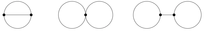
[image:13.595.92.517.410.479.2]

Let us first consider the purely bosonic sector. As pointed out in section 4, the spectrum of the theory contains one real boson of squared mass 1, one real boson of squared mass 1₂ and three complex massless bosons. The interaction among these excitations involves cubic and quartic ver-tices which give rise to the diagrams in figure5.1.

Figure 1: Sunset, double bubble and double tadpole are the diagrams appearing in the two-loop contribution to the partition function.

We observe that the AdS light-cone gauge Lagrangian contains only diagonal bosonic propaga-tors, which introduces considerable simplifications in the perturbative computation. The explicit expressions of the propagators are

Gϕϕ(p) =

1

p2_{+ 1} Gzaz¯b(p) =

2δb a

p2 Gx1x1(p) =

1

p2₊1 2

. (5.2)

The cubic interactions involving only bosonic fields are of three different kinds

Vϕx1_x1 =−4ϕ

(∂s−1₂)x1

2

Vϕ3 = 2ϕ

(∂tϕ)2−(∂sϕ)2

Vϕ|z|2 = 2ϕ

|∂tz|2− |∂sz|2

.

(explicit reductions for the relevant integrals are spelled out in appendixC)

I m2 ≡

Z d2p

(2π)2 1

p2_+m2 (5.4)

I m2₁, m2₂, m2₃ ≡

Z

d2p d2q d2r

(2π)4

δ(2)(p+q+r) (p2_+m2

1)(q2+m22)(r2+m23)

. (5.5)

The latter integral is finite, provided none of the masses vanishes, and is otherwise IR divergent. The former is clearly UV logarithmically divergent, and also develops IR singularities in the mass-less case. In our computation we expect all UV divergences to cancel and therefore no divergent integral to appear in the final result. Nonetheless, performing reduction of potentially divergent tensor integrals to scalar ones still implies the choice of a regularization scheme. In our case we use the one adopted in [42,51,78]. This prescription consists of performing all manipulations in the numerators in d= 2, which has the advantage of simpler tensor integral reductions. In this process we set to zero power UV divergent massless tadpoles, as in dimensional regularization

Z d2p

(2π)2 p 2n

= 0, n_≥0. (5.6)

All remaining logarithmically divergent integrals happen to cancel out in the computation and there is no need to pick up an explicit regularization scheme to compute them.

As an explicit example, we consider the contribution to the sunset coming from the first vertex in (5.3)

−1 2hV

2

ϕx1_x1i=−

Z

d2p d2q d2r

(2π)4

(1 + 4q2₁) (1 + 4r₁2)δ(2)(p+q+r) (p2_{+ 1)(q}2₊1

2)(r2+12)

= 1 2I 1,

1 2,12

. (5.7)

The reason why the coefficient of the integral in the second term of (5.7) is exactly (−1) is the topic of section 5.4. We note that the integral I 1,1₂,1₂

already appeared in [42] and is a particular case of the general class

I 2m2, m2, m2

= K

8π2_m2 , (5.8)

whereK is the Catalan constant

K ≡ ∞ X

n=0

(−1)n

(2n+ 1)2 . (5.9)

The contribution of the sunset diagram involving the second vertex in (5.3) is proportional to

I(1)2, whereas the contribution of the third vertex vanishes

−1 2hV

2

ϕ3i= 2I(1)2 −

1 2hV

2

ϕ|z|2i= 0 (5.10)

The final contribution of the bosonic sunset diagrams is

W2,bos. sunset=

1 2I 1,

1 2,

1 2

+ 2I(1)2. (5.11)

Next we consider bosonic double bubble diagrams. The relevant quartic vertices are

Vϕ2_x1_x1 = 16ϕ2

(∂s−1₂)x1

2

(5.12)

Vϕ4 = 4ϕ2

(∂tϕ)2+ (∂sϕ)2+

1 6ϕ

2

(5.13)

Vϕ2_|z|2 = 4ϕ2

|∂tz|2+|∂sz|2

(5.14)

Vz4 =

1 6

h

(¯za∂tza)2+ (¯za∂sza)2+ (za∂t¯za)2+ (za∂s¯za)2

−|z|2 |∂tz|2+|∂sz|2

− |z¯a∂tza|2− |¯za∂sza|2

i

. (5.15)

Despite the lengthy expressions of the vertices, the only non-vanishing contribution comes from

V_ϕ4 and gives

W2,bos. bubble=−2I(1)2 (5.16)

and cancels the divergent part of (5.11). As a result, the bosonic sector turns out to be free of divergences without the need of fermonic contributions, which was already observed in the

AdS5×S5 case [42].

5.2 Fermionic contributions

We compute the diagrams arising from interactions involving fermions. The fermionic propagators can be read from the inverse of the kinetic matrix KF (4.3)

Gη4η¯4(p) =Gθ4θ¯4(p) =

p0

p2 Gη4θ¯4(p) =Gθ4η¯4(−p) =−

p1

p2

Gηaη¯b(p) =Gθaθ¯b(p) =

p0

p2₊1 4

δab Gηaθ¯b(p) =Gθaη¯b(−p) =−

p1+₂i

p2₊1 4

δab (5.17)

The main difference between the spectrum of AdS5 ×S5 and the one introduced in section 4

resides in the fermionic part. Although both theories have eight fermionic degrees of freedom, in

AdS4×CP3they are split into six massive and two massless excitations, which interact non-trivially

among themselves.

We start by considering diagrams involving at least one massless fermion. The relevant cubic vertices are (we denote byψ the fermionsη andθ collectively)

Vzηaη4 = −2∂tz

a_η

aη4+h.c. Vzηaθ4 = 2∂sz

a_η

aθ4−h.c.

V_ϕη4θ¯4 =−2i ϕ(¯θ4∂sη4−∂sθ¯4η4)−h.c. Vx1ψ¯4_ψ

4 =−2i(¯η

4_η

4+ ¯θ4θ4)(∂s−1₂)x1. (5.18)

The quartic interactions are either not suitable for constructing a double tadpole diagram or they produce vanishing integrals. These include vector massless tadpoles, which vanish by parity, and tensor massless tadpoles, which have power UV divergences and are set to zero. For completeness we list them in appendixB.

Focussing on the Feynman graphs which can be constructed from cubic interaction we also note that the only double tadpole diagrams that can be produced using (5.18) involve tensor massless tadpole integrals and therefore vanish. In the sector with massless fermions we are therefore left with the sunset diagrams, which, thanks to the diagonal structure of the bosonic propagators, turn out to be only five

W2,ψ4 =−

1

2hVzηaη4Vzηaη4 +Vzηaθ4Vzηaθ4 + 2Vzηaη4Vzηaθ4+Vϕη4θ¯4Vϕη4θ¯4 +Vx1ψ¯4ψ4Vx1ψ¯4ψ4i.

The explicit computation of the individual contributions shows that they are all vanishing. As an example we consider

− 1₂hV_ϕη4θ¯4V_ϕη

4θ¯4i= 4

Z

d2p d2q d2r

(2π)4

(p1−q1)2(p0q0−p1q1)δ(2)(p+q+r)

p2_q2_(r2_{+ 1)} = 0 (5.20)

and similar cancellations happen for the other diagrams. Therefore we conclude that W2,ψ4 = 0

and that massless fermions are effectively decoupled at two loops.

We then move to consider massive fermions, starting from their cubic coupling to bosons

Vzηη =−ǫabc∂tz¯aηbηc+h.c. Vzηθ =−2ǫabcz¯aηb(∂s− 1₂)θc−h.c.

Vϕηθ =−4i ϕ ηa(∂s−1₂)¯θa−h.c. Vx1_ηη =−4iη¯aη_a(∂_s−1

2)x

1_{. (5.21)}

Precisely as in the massless case, this generates five possible sunset diagrams. None of them is vanishing. We present the details of a particularly relevant example, i.e. the one involving the vertex Vx1_ηη. This gives

−1₂hVx1_ηηV_x1_ηηi= 24

Z

d2p d2q d2r

(2π)4

(p2₁+1₄)q0r0δ(2)(p+q+r)

(p2₊1

2)(q2+14)(r2+14)

=₋3 8I

1 2,14,14

+3

4I

1 4

2 .

(5.22)

We note the appearance of another integral in the class (5.8). The coefficient in front of this integral depends on the degrees of freedom of the theory and is thoroughly discussed in section (5.4). The partial results of the remaining sunset diagrams are

−1

2h(Vzηη+Vzηθ)(Vzηη+Vzηθ)i= 3I

1 4

2

−6I 1₄ I(0)

−1₂hVϕηθVϕηθi_1PI= 6I 1₄

I(1) + 3 4I

1 4

2

. (5.23)

The latter vertices can be contracted also in a non-1PI manner

−1

2hVϕηθVϕηθinon-1PI =−

1

2Gϕϕ(0)×2

6_×32_×Z d2p

(2π)2

p2₁+1₄

p2₊1 4

=−9 2I

1 4

2

(5.24)

where the factor in front of the integrals comes from the expression of the vertex and from counting the degrees of freedoms that can run in the loops. As in [42], the divergent contribution proportional to I 1₄2

cancels exactly those coming from (5.22) and (5.23). The total cubic fermionic part reads

W2,ferm. cubic =−

3 8I

1 2,14,14

+ 6I 1₄

I(1)₋6I 1₄

I(0). (5.25)

Finally we consider the fermionic double bubble diagrams. These involve the fermionic quartic vertices. However, most of the vertices appearing in the Lagrangian cannot contribute to the partition function either because the bosonic propagators are diagonal or because they would produce vanishing integrals. We present the whole list of quartic vertices in appendix B and we spell out here only the relevant ones for our computation

Vϕ2_ηθ= 8i ϕ2η_a(∂_s−1

2)¯θ

a_{−h.c. V}

zzηθ=−2i

h

|z|2ηa(∂s−1₂)¯θa−z¯bzaηa(∂s−1₂)¯θb

i

−h.c. .

Although we can build a diagram withVη4, fermion propagators carry one component of the loop

momentum in the numerator and produce vector tadpole integrals, which vanish by parity. We conclude that the contribution from fermionic double bubble graphs is

W2,ferm. bubbles =−6I 1₄

I(1) + 6I 1₄

I(0). (5.27)

Summing all the partial results and reinstating the dependence on the string tension and the volume, we obtain

W2 =

V2

T

1 2I 1,

1 2,12

−3

8I

1 2,14,14

=−1 4

V2

T I 1,

1 2,12

=− K 16π2

V2

T (5.28)

where T is defined in (1.5). Finally we can plug this expression into equation (3.9) and read out the second order of the strong coupling expansion (3.10) of the ABJM cusp anomalous dimension

a2 =−

K

4π2. (5.29)

5.3 The cusp anomalous dimension

We summarize the results of our superstring computation, presenting the strong coupling expansion of the ABJM cusp anomalous dimension up to two-loop order. Reinstating the definition of the string tension (1.5) in terms of the ABJM ’t Hooft coupling and plugging (4.7) and (5.29) into (3.10), we find

fABJ M(λ) =

√

2λ−5 log 2 2π −

K

4π2 +

1 24

1 √

2λ+O λ

−1

, (5.30)

which is the main result of the paper. From the string dual point of view it looks convenient to define the shifted coupling

˜

λ_≡λ₋ 1

24, (5.31)

in terms of which we can rewrite the scaling function more compactly as

fABJ M

˜

λ=p2˜λ₋5 log 2

2π − K

4π2p_2˜λ+O

˜

λ−1. (5.32)

5.4 Comparison with AdS_5×S5

In this section we point out similarities and differences between the calculation we performed and itsAdS5×S5analogue [42]. The starting points, i.e. the Lagrangians inAdSlight-cone gauge, look

rather different. Yet the final results of the two-loop computations are strikingly similar. More precisely, when written in terms of the string tension, the two expressions have exactly the same structure up to the numerical coefficients in front of the integrals. Indeed the AdS5 computation

gives

W(AdS5)

2 =

V2

T

1 4I 1,

1 2,12

−1₄I 1₂,1₄,1₄

, (5.33)

which looks very similar in structure to (5.28). Furthermore, using (5.8), both combinations sum up to

W2 =−

V2

T

1 4I 1,

1 2,12

and only the different relation between the string tension and the ’t Hooft couplings distinguishes the final results. It is easy to trace the origin of the integrals and their coefficients back in the vertices of the Lagrangian and to understand their meaning. In particular in both computations only the sunset diagrams involving the interactions Vϕxx and Vxψψ (with massive fermions) seem

to effectively contribute. All other terms are also important, but just serve to cancel divergences. Hence we can now focus on the relevant interactions and point out the differences between the

AdS5 and theAdS4 cases.

We start from the bosonic sectors. The two theories differ for the number of scalar degrees of freedom with given masses. Focussing on massive fluctuations, after gauge fixing we have one scalar with m2 = 1 associated to the radial coordinate of AdSd+1 and (d−2) real scalars with

m2 ₌ 1

2. In the metric we chose for the AdS4 ×CP3 background, the size of the AdS4 part is

rescaled by a factor ofr2 _{= 4. We have compensated this, parametrizing the radial coordinate as}

w=erϕ and introducing a factor r in the fluctuation of x1, so as to have the same normalization for their kinetic terms as inAdS5×S5. This causes some factorsr to appear in interaction vertices

in our Lagrangian. Apart from this, the relevant interaction vertices are exactly the same. Then, the number ofx fields (d−2) and this factorr determine the coefficient of the integral I 1,1₂,1₂ appearing in equations (5.28) and (5.33).

Turning to fermions, the first striking difference between theAdS5 and AdS4 cases is the presence

of massless ones. As pointed out at the beginning of section 5.2 their contribution is effectively vanishing at two loops (though they do contribute at first order). Focussing on massive fermions, the relevant cubic interactions giving rise to I 1₂,1₄,1₄

look again similar in theAdS4 and AdS5

cases. The difference is given once more by the ratio of the radiir (through the normalization ofϕ

andx coordinates) and the numbernf of massive fermions in the spectrum (nf = 8 forAdS5×S5

and nf = 6 for AdS4×CP3).

The final results (5.28) and (5.33) can be re-expressed in the general form

W(AdSd+1)

2 =

V2

T

(d₋2)r2

8 h

I 1,1₂,1₂ −nf

8 I

1 2,14,14

i

= V2

T

(d₋2)r2

8

1₋nf 4

I 1,1₂,1₂

, d= 3,4, (5.35)

where the cases at hand are d= 4, nf = 8, r = 1 forN = 4 SYM and d= 3, nf = 6, r = 2 for

ABJM.

6

Concluding remarks

In this work we have computed the cusp anomalous dimension of ABJM theory up to second order in its strong coupling expansion. This result has been determined considering theAdS4×CP3 κ

-symmetry gauge-fixed action of [45,46] and studying its fluctuations about the null cusp background (3.1), which is a classical solution thereof. As in theAdS5×S5 counterpart of this calculation [42],

theAdSlight-cone gauge approach [49] makes the explicit evaluation rather manageable, allowing us to push the expansion of the string partition function up to second order.

While at one loop we confirm a known result [28,32,36], at two-loops we provide a new im-portant piece of data, see (1.6), which we combine with a proposal based on the Bethe Ansatz of AdS4/CFT3 [4] to give our two-loop correction to the so-called interpolating function h(λ) of

perturbation theory we must implement in our calculation a “correction” to the string tension in terms of the ’t Hooft coupling, which was pointed out in [64] to be due to higher order corrections (in curvature) to the background. We show that the strong coupling two-loop correction for h(λ) is only due to the anomalous shift of the curvature radius in the Type IIA description [64]. This supports the observation in [66] on the origin of the shift appearing in its proposal (1.13), which knows nothing about the gravity side but coincides in fact with the correction of [64].

In perspective, we observe that the light-cone gauge approach could be pushed to a much stronger check of (1.11), by testing its finite coupling regime. Following [79], one could discretize the light-cone Lagrangian (3.4), put it on a lattice and perform numerical simulations to determine the ABJM scaling function in terms of the coupling constant, for any value thereof. By comparison with the same results for N = 4 SYM one could then provide numerical values of h(λ) at some finite values ofλ, which could then be contrasted with (1.11).

The manifest cancellation of UV divergences that we find here provides a direct demonstra-tion of the quantum consistency of the AdS4×CP3 action of [45,46], and shows that it can be

readily used for non-trivial strong coupling computations in theAdS4/CFT3 framework (following

for example [52,53]). In particular, the consistency of the result with predictions coming from integrability, the conjecture [66] and the “corrected” dictionary of [64] can be taken as evidence, albeit indirect, of quantum integrability for the Type IIAAdS4×CP3 superstring in this gauge.

Acknowledgments

It is a pleasure to thank Alessandra Cagnazzo, Andrea Cavagli`a, Ben Hoare, Valentina G.M.Puletti, Nikolay Gromov, Radu Roiban, Roberto Tateo and Arkady Tseytlin for discussions, and in par-ticular Ben Hoare for useful comments on the draft. The work of LB, AB, VF and EV is funded by DFG via the Emmy Noether Program “Gauge Fields from Strings”.

A

Lagrangian in the Wess-Zumino type parametrization

In this appendix we rewrite the Lagrangian (2.5) in a form that resembles the Wess-Zumino type parametrization introduced in [49], and compare it to theAdS5×S5case. In [49] the authors found

two possible ways to eliminate the fermion rotation (2.12), either by a change of parametrization for S5 or by the introduction of a covariant derivative for the terms quadratic in fermions. Here we explore only the second option and we leave the first one for future development. We first introduce a collective index for upper and lower indices so that

ηˆa=

ηa

¯

ηa

. (A.1)

In this notation the action of the matrixT on the fermions (2.12) can be rewritten as

ˆ

ηˆa=Tˆa ˆ_b

ηˆb (A.2)

where the matrix T_ˆa ˆ_b

is given in (2.17). We also introduce the shorthand notation

whereηˆa_{= (¯η}a_{, η}

a). In [49] a recipe for going from the Killing parametrization to a Wess-Zumino

type gauge was given, which consists of rotating back the fermions. This generates additional terms coming from derivatives that can be reabsorbed into a covariant derivative. In particular, we apply the transformation

ηaˆ→ T−1

ˆb

ˆ

aηˆb. (A.4)

In contrast with the AdS5 ×S5 case the matrix T is not block diagonal, therefore one has

ηˆa∂iηˆa= ˆηˆa∂ˆiηaˆ, where it is crucial to use hatted indices. This transformation removes all the hats

from fermions, at the price of introducing the covariant derivative

D=d₋Ω, (A.5)

where Ω≡Ωˆa ˆ b _=dT

ˆ

aˆc(T−1)ˆc ˆ b

and dΩ−Ω∧Ω = 0. More explicitly16, the (matrix) Cartan form entering the definition of the (dimensionally reduced) supercoset element reads

Ωˆa ˆ b _=i

Ω b

a −δbaΩcc ǫacbΩc

−ǫacb_Ω

c −Ωa_b+δ_baΩcc

, (A.6)

with components given by

Ω_ab =i(1−cos|z|)

|z|2 (¯zadz b

−dz¯azb)−iz¯azb

(1₋cos_|z_|)2

2|z|4 (dz c_¯z

c−zcdz¯c), (A.7)

Ωa=dz¯a

sin_|z_|

|z| + ¯za

sin_|z_|(1₋cos_|z_|) 2|z|3 (dz

c_z¯

c−zcdz¯c) + ¯za

1 |z| −

sin_|z_|

|z|2

d_|z_|, (A.8)

Ωa=dzasin|z|

|z| +z

asin|z|(1−cos|z|)

2|z|3 (z c_dz¯

c−dzcz¯c) +za

1 |z|−

sin_|z_|

|z|2

d|z|. (A.9)

Above, Ωcc is the trace of (A.7) and is related to ˜Ωcc defined in (2.16) via ˜Ωcc = 2 Ωcc.

We can also decompose the matrix Ω in order to separate the contributions from the vielbein and from the spin connection17

Ωˆa ˆ

b _{= Ω}cˆ_(E ˆ c)aˆ

ˆ b_{+ Ω}c

d(Jcd)ˆa ˆ b

(A.10)

with18

(Eˆc)aˆ ˆ b _=i

0 ǫacb

−ǫacb ₀

(J_cd)ˆa ˆ_b

=i

δd

aδbc−δbaδdc 0

0 ₋δd

bδac +δbaδcd

. (A.12)

This decomposition provides a way to project out the spin connection and find the exact relation between the vielbein Ωˆa and the matrix Ω

Ωcˆ=

1

2Tr(EˆcΩ) . (A.13)

16_{The matrix Ω was already introduced in [76] however there it was defined as Ω} ˆ a

ˆb_=iT

ˆ acˆdT−1ˆc

ˆ b

=₋idTˆacˆT−1ˆc ˆ b

, differing from ours by a factor ofi. To make contact with the expressions of [76] we add such a factor in formula (A.6).

17_{A similar procedure was applied in [49] where in that case the decomposition is expressed in terms of theSO(5)}

γ-matrices.

18_{Let us stress that the meaning of the first term of equation (A.10) in matrix form is the following}

Ωcˆ

(Eˆc)ˆa

ˆb

=

Ωc_(E

c)ab+ Ωc(Ec)ab Ωc(Ec)ab+ Ωc(Ec)ab

Ωc_(E

c)ab+ Ωc(Ec)ab Ωc(Ec)a_b+ Ωc(Ec)a_b

(A.11)

and the explicit expression of (Ecˆ)ˆa ˆ b

After having introduced all the necessary ingredients, we are ready to rewrite the Lagrangian in a form which resembles theAdS5×S5 case. We separate it into

L=LB+L(2)_F +L(4)_F (A.14)

where the bosonic contribution is simply given by the standard bosonic sigma model withAdS4× CP3 _{as target space}

LB=γij

e−4ϕ

4 ∂ix

+_∂

jx−+∂ix1∂jx1

+∂iϕ∂jϕ+ ΩaiΩaj

(A.15)

where the vielbein Ωa

i are defined in the natural way Ωa = Ωaidσi with σi = (τ, σ). Notice also

that Ωˆa

iΩajˆ = 2 ΩaiΩaj for the symmetry of the worldsheet metric. The quadratic part in the

fermion fields can be expressed as

L(2)_F =−2e−4ϕ∂ix+

hi

2γ

ij _ηˆa_D

jηˆa+θˆaDjθˆa−2 ΩˆcjηEˆcη

+εijηˆaCˆa ˆ b _D

jθˆb+e− 2ϕ_η

ˆb∂jx 1₎

+i 2γ

ij _η¯4_∂

jη4+ ¯θ4∂jθ4−4i ηaΩajη4+ 2iΩa ja Θ−h.c.

+1 2ε

ij _η¯4_∂

jθ4−θ¯4∂jη4+ 4i ηaΩajθ4+ 2iΩa ja Θ˜ −e−2ϕΘ∂jx1+h.c.

i .

(A.16)

Here we have introduced the charge conjugation matrix C, given explicitly by19

Cˆa ˆ b ₌

δba 0

0 ₋δa b

, (A.17)

and the combinations Θ = θ4θ¯4 +η4η¯4 and ˜Θ = θ4η¯4 −η4θ¯4. The first line of this Lagrangian

(A.16) closely resembles expression (1.6) of [49], that is theAdS5×S5 Lagrangian in Wess-Zumino

type parametrization. This is the part of the Lagrangian that does not contain the fermions η4

and θ4, which emerge [45] when obtaining the AdS4×CP3 action from dimensional reduction of

the AdS4 ×S7 supermembrane action. The main difference with respect to AdS5 ×S5 is that

theSU(4) R-symmetry is not explicitly realized on the fermionic Lagrangian (A.16). This feature is inherited by the quantum fluctuations around the light-like cusp. As a result of the broken symmetry, the spectrum contains fermionic degrees of freedom with different masses (one gets 6 massive and 2 massless excitations). Our one- and two-loop calculations have explicitly shown that the role of the massless fermions (˜η4 and ˜θ4) is crucial for compensating the bosonic degrees

of freedom, making the one-loop partition function UV-finite. At two loops their interactions with the other excitations would in principle start playing a part. Nevertheless it turns out that the massless fermions decouple from the computation and do not contribute to the two-loop result.

The last term of the superstring Lagrangian is quartic in fermions

L(4)_F = 4e−8ϕγij∂ix+∂jx+[(ηaη¯a)2+ 2εabcηaηbηcη4+ 2η4η¯4ηaη¯a−Θ2+h.c.]. (A.18)

As discussed for the quadratic part, the first terms clearly reminds the expression for AdS5×S5

(equation (1.10) of [49]), whereas the others contain the non-trivial interactions ofη4 and θ4.

19_{The fact that the matrix is diagonal and not anti-diagonal is a consequence of our conventions for grouping the}

spinors. Notice also that for our conventionsηˆa_η ˆ

a= 0 whereasηaˆCˆa ˆ b_η

ˆ

B

Details on the expanded Lagrangian

In this appendix we provide the details of the Lagrangian (3.4) expanded up to quartic order. As in section5we list the vertices as they appear in_Lint, namely with an extra factor 1₂ with respect

to the original Lagrangian. We drop tildas, understanding that we are dealing with the fluctuation fields of (3.4). The cubic vertices are

Vϕx1_x1 =−4ϕ

(∂s−1₂)x1

2

Vϕ3 = 2ϕ

(∂tϕ)2−(∂sϕ)2

Vϕ|z|2 = 2ϕ

|∂tz|2− |∂sz|2

Vzηη=−ǫabc∂tz¯aηbηc+h.c. Vzηθ =−2ǫabcz¯aηb(∂s−1₂)θc−h.c.

Vϕηθ =−4i ϕ ηa(∂s−1₂)¯θa−h.c. Vx1_ηη =−4iη¯aη_a(∂_s− 1

2)x 1

Vzηaη4 = −2∂tz

a_η

aη4+h.c. Vzηaθ4 = 2∂sz

a_η

aθ4−h.c.

V_ϕη4θ¯4 =−2i ϕ(¯θ4∂sη4−∂sθ¯4η4)−h.c. Vx1_ψ¯4_ψ

4 =−2i(¯η

4_η

4+ ¯θ4θ4)(∂s− 1₂)x1 (B.1)

The quartic vertices read

Vz4 =

1 6

h

(¯za∂tza)2+ (¯za∂sza)2+ (za∂tz¯a)2+ (za∂sz¯a)2

−|z|2 |∂tz|2+|∂sz|2

− |z¯a∂tza|2− |z¯a∂sza|2

i

(B.2)

Vϕ2_x1_x1 = 16ϕ2

(∂s− 1₂)x1

2

Vϕ4 = 4ϕ2

(∂tϕ)2+ (∂sϕ)2+

1 6ϕ

2

(B.3)

V_ϕ2_|z|2 = 4ϕ2

|∂tz|2+|∂sz|2

V_z¯˙zψ¯4_ψ

4 =−2i(¯η

4_η

4+ ¯θ4θ4)¯zb∂tzb+h.c. (B.4)

Vη2_η

4η¯4 = 8 ¯η

4_η

4η¯aηa Vz′_¯zψ¯4_ψ

4 =−2i(¯η

4_θ

4−θ¯4η4)¯zb∂szb−h.c. (B.5)

V_η4 = 4(¯ηaηa)2 Vϕ2_η

4θ¯4 = 4i ϕ

2_(¯θ4_∂

sη4−∂sθ¯4η4)−h.c. (B.6)

V_η

4¯η4θ4θ¯4 =−8 ¯η

4_η

4θ¯4θ4 Vϕ x1_ψ¯4_ψ

4 = 12i ϕ(¯η

4_η

4+ ¯θ4θ4)(∂s−1₂)x1 (B.7)

Vη3_η

4 = 4ǫ

abc_η

aηbηcη4+h.c. Vzzη¯a_η

4 =−2i ǫabc∂tz

a_zb_η¯c_η

4+h.c. (B.8)

Vϕ zηaθ4 =−8ϕ ∂sz

a_η

aθ4−h.c. Vϕ zηθ = 8ϕǫabcz¯aηb(∂s− 1₂)θc−h.c. (B.9)

Vzzη¯a_θ

4 = 2i ǫabc∂sz

a_zb_η¯c_θ

4−h.c. Vzzηη =−2i(¯za∂tzaη¯bηb−z¯b∂tzaη¯bηa) +h.c. (B.10)

Vϕ x1_ηη = 24i ϕη¯aη_a(∂_s−1

2)x

1 _V

zzηθ =−2i[|z|2ηa(∂s−1₂)¯θa−z¯bzaηa(∂s−1₂)¯θb]−h.c.

(B.11)

Vϕ2_ηθ = 8i ϕ2η_a(∂_s−1

2)¯θ a

−h.c. Vx1_zηη =−4 (∂_s−1

2)x1ǫ abc_z¯

aηbηc−h.c. (B.12)

C

Integral reductions

In this appendix we provide the relevant tensor integral reductions in two dimensions that we used in the computation of the two-loop correction to the partition function. We define the two basic scalar integrals

I m2 ≡

Z d2p

(2π)2 1

p2_+m2 (C.1)

I m2₁, m2₂, m2₃ ≡

Z _d2_{p d}2_{q d}2_r (2π)4

δ(2)_(p+q+r)

(p2_+m2

1)(q2+m22)(r2+m23)

Then we have (the factors (2π)4 in the denominator of the integrands are understood)

Z

d2p d2q d2r pµ_qν_δ(2)_(p+q+r)

(p2_+m2

1)(q2+m22)(r2+m23)

= (C.3)

= δ

µν

4

I(m2₁)I(m2₂)−I(m2₁)I(m2₃)−I(m2₂)I(m2₃) + (m2₁+m2₂−m₃2)I(m2₁, m2₂;m2₃)

(C.4)

I_µµ(m2₁, m2₂;m2₃) = Z

d2p d2q d2r (p_·q)δ(2)(p+q+r) (p2_+m2

1)(q2+m22)(r2+m23)

= (C.5)

= 1 2

I(m2₁)I(m2₂)−I(m2₁)I(m2₃)−I(m2₂)I(m2₃) + (m2₁+m2₂−m₃2)I(m2₁, m2₂;m2₃)

(C.6)

Z

d2p d2q d2r pµ_pν_δ(2)_(p+q+r)

(p2_+m2

1)(q2+m22)(r2+m23)

= δ

µν

2

I(m2₂)I(m2₃)₋m₁2I(m2₁, m2₂;m2₃)

(C.7)

J _≡ Z

d2p d2q d2r p2q2δ(2)(p+q+r) (p2_+m2

1)(q2+m22)(r2+m23)

=m2₁m2₂I(m2₁, m2₂;m2₃)₋m2₁I(m2₁)I(m2₃)₋m₂2I(m2₂)I(m2₃)

(C.8)

K _≡ Z

d2p d2q d2r(p_·q)2δ(2)(p+q+r) (p2_+m2

1)(q2+m22)(r2+m23)

= 1 2

−m2₂I(m2₂)I(m2₃)₋m2₁I(m2₁)I(m2₃)+

+(m2₁+m2₂−m2₃)I_µµ(m2₁, m2₂;m2₃)

(C.9)

Z

d2_{p d}2_{q d}2_{r p}µ_pν_qρ_qσ_δ(2)_(p+q+r)

(p2_+m2

1)(q2+m22)(r2+m23)

=

3 8J−

1 4K

δµνδρσ+

1 4K−

1 8J

(δµρδνσ +δµσδνρ) (C.10)

Z

d2_{p d}2_{q d}2_{r p}µ_pν_pρ_qσ_δ(2)_(p+q+r)

(p2_+m2

1)(q2+m22)(r2+m23)

= 1 8(δ

µν_δρσ_+δµρ_δνσ_+δµσ_δνρ₎

m2₂I(m2₂)I(m2₃)−m2₁I_µµ(m2₁, m2₂;m2₃)

(C.11)

L_≡ Z

d2p d2q d2r p2 (q_·r) δ(2)(p+q+r) (p2_+m2

1)(q2+m22)(r2+m23)

=₋m2₁I_µµ(m2₃, m2₂;m2₁) (C.12)

M _≡

Z _d2_{p d}2_{q d}2_r(p

·q)(p_·r)δ(2)_(p+q+r)

(p2_+m2

1)(q2+m22)(r2+m23)

= 1 2

(m2₁+m2₃₋m2₂)I_µµ(m2₁, m2₂;m2₃)+ +m2₁I(m2₁)I(m2₃)₋m2₂I(m2₂)I(m2₃)

(C.13)

Z

d2p d2q d2r pµ_pν_qρ_rσ_δ(2)_(p+q+r)

(p2_+m2

1)(q2+m22)(r2+m23)

=

3 8L−

1 4M

δµνδρσ+

1 4M −

1 8L

(δµρδνσ+δµσδνρ).

(C.14)

References

[1] O. Aharony, O. Bergman, D. L. Jafferis and J. Maldacena,“_N = 6 superconformal

Chern-Simons-matter theories, M2-branes and their gravity duals”,JHEP 0810, 091 (2008),

arXiv:0806.1218.

[2] J. M. Maldacena,“The Large N limit of superconformal field theories and supergravity”,

Adv.Theor.Math.Phys. 2, 231 (1998),hep-th/9711200.

[3] J. Minahan and K. Zarembo,“The Bethe ansatz for superconformal Chern-Simons”,

JHEP 0809, 040 (2008),arXiv:0806.3951.

[4] N. Gromov and P. Vieira,“The all loop AdS4/CFT3 Bethe ansatz”,JHEP 0901, 016 (2009),