Munich Personal RePEc Archive
Optimal monetary policy and default
Lizarazo, Sandra and Da-Rocha, Jose-Maria
ITAM, Universidade de Vigo
29 June 2011
Optimal Monetary Policy and Default
Sandra Lizarazo
ITAM
Jos´e-Mar´ıa Da-Rocha
Universidade de Vigo
June 29, 2011
Abstract
In a context in which individuals might default on their debts and subsequently be excluded from credit markets, holding money helps agents smooth their consumption during periods in which they cannot borrow. Therefore holding money makes the punishment to default less severe. In this context, by affecting money demand, monetary policy can affect incentives to default; determining optimal monetary policy can then be thought of as equivalent to choosing the optimal default rate. Since each economy might have a different optimal default rate, each economy might have a different optimal monetary policy different from the Friedman rule. Specifically, we compare the US to Colombia, using a model with idiosyncratic labor income risk and fiat money. Given differences in enforcement of debt contracts, and differences in income variability and persistence, we find that high inflation is costlier for developing countries compared to developed countries.
Keywords: Default, Inflation, Fiat Money, Friedman rule, Endogenous Borrowing Con-straints, Precautionary Savings.
JELClassification: E21; E41; E44; E52
We are grateful in non particular order to George Alessandria, Jonathan Heathcote, Timothy J. Kehoe, Igor Livshits, Pablo Andres Neumeyer, Martin Uribe for their discussions and suggestions. We also thank the comments of seminar participants at the Macro Dynamic Workshop of Vigo, and the XI Workshop in International Economics and Finance. All remaining errors are our own.
1
Introduction
Determination of the optimal monetary policy is a recurrent subject in economic theory. The current literature generally approaches the question from the point of view of transaction costs and purchasing power. The current paper looks at this question from a new perspective by considering the interaction between monetary policy and the frequency of default on debt contracts. The question is explored using a standard heterogeneous agents economy, with idiosyncratic labor income uncertainty, and incomplete credit markets.
In the economy in this paper, individuals use two different assets to smooth con-sumption: one period non-contingent bonds and fiat money. Due to limited commit-ment, individuals might default on their debts, and as punishment they are excluded from credit markets for a number of periods. If money cannot be liquidated to pay the defaulters’ debts, then money can be used by the individuals to transfer resources from periods of participation in credit markets towards periods of exclusion from credit markets.1 Furthermore, during the periods of exclusion from credit markets money can also be used to self-insure. In this context money facilitates default.
Because monetary policy changes the return to money balances (i.e. the inflation rate), it has an effect in money demand, and therefore on the costs of defaulting in the economy. High inflation rates tend to make costlier to hold money, and have the effect of making the punishment for default more severe. The opposite holds true for low inflation rates. As a consequence, monetary policy has an important role in modifying the incentives to default in the economy. By setting a relative high (low) level of inflation, monetary authorities can strengthen (weaken) the punishment for default. In this way monetary policy might reduce (increase) the occurrence of default at equilibrium. As a result, in this economy the determination of the optimal monetary policy is tightly linked to the determination of the optimal frequency of default.
It is interesting to note that at equilibrium, the welfare impact of a higher fre-quency of default is economy dependent. That is, a higher frefre-quency of default can be welfare increasing for some economies and welfare decreasing for other economies. The logic behind this result stems from the fact that default can be seen as an alter-native tool to precautionary savings for self-insuring. As discussed in Zame (1993), default has a role in completing credit markets and enhancing the efficiency of the
1The assumption of not liquidating the defaulter’s money is important and can be justified to
allocations in the economy, by making non contingent assets (i.e. the bonds) act as de facto contingent assets in some instances. On the other hand, higher frequency of default increases the riskiness of lending in the economy, and makes it harder to observe large levels of debt at equilibrium. As a consequence, individuals face tighter credit constraints. Other things equal, this effect reduces the usefulness of credit markets for self-insuring.
The tension between these two possible effects implies that the optimal monetary policy should be one that does not minimize the possibilities of borrowing but also does not minimize the possibilities of defaulting. Because the highest possible fre-quency of default at equilibrium is associated with the Friedman rule, this policy is not optimal in general.2 On the other hand, because the lowest possible frequency of default at equilibrium is associated with an infinite inflation rate, a policy with infinite inflation is also non-optimal.3 As will be demonstrated in this paper, under very plausible circumstances, the optimal inflation rate is positive and not too high. Furthermore the optimal inflation rate is highly dependent on the characteristics of the economy. In the numerical simulations of the paper, we find that high inflation is costlier in terms of welfare for countries in Latin America, like Colombia, where enforcement of debt contracts is weak and income variability and persistence are high than it is in more developed countries, like the United States.
Regarding the quantitative results of the paper, it is worth mentioning that by looking at money only as a medium to store wealth and ignoring the transactional role of money in the economy, we may underestimate the inflation costs in the economy. This seems particularly true when we look at our result for the optimal inflation rate for the United States, which looks too high. Surely modeling the transactional role of money would produce a more reasonable estimate. Instead, the current paper focuses on the qualitative message of the current model. That is, in addition to its more obvious effects, monetary policy can also influence welfare through its effect on the incentives to default. Ignoring the other functions of money helps us to focus completely on this new aspect of monetary policy that has previously been overlooked. Theoretically, a nice feature of the model is that it supports fiat money at
equilib-2In general the Friedman rule is not optimal because it is consistent with a very low amount
of debt at equilibrium. This low debt is reflected in very tight credit constraints: when money earns the same return as bonds, individuals can use money to move resources in a very efficient way from the period in which they default to the periods of credit market exclusion. In this way the reputation-based punishment for default is completely destroyed. Therefore, as Bulow and Rogoff (1989) demonstrate, it is impossible to support debt at equilibrium based purely on the reputation of the borrower. In this case debt can only be supported if there are other punishments to default.
3In contrast to the negative inflation of the Friedman rule, if inflation is infinite, the punishment
rium without the need of imposing exogenous ad-hoc credit constraints (as in Bewley (1980,1983)) or exogenous timing frictions in the bond markets (as in Akyol (2004)) to induce individuals in the economy to demand money. Under the current frame-work, as long as individuals’ probability of default is non-zero, some agents (those at the verge of default or the ones that have recently defaulted) would hold some money even when fiat money is a dominated asset in terms of its return in comparison to bonds.4
Another important feature of the current model is that the pattern of money holdings at equilibrium is consistent with the pattern observed in practice. This pattern suggests that the least wealthy agents hold a relatively larger proportion of their wealth in liquid assets than the wealthier agents in the economy. Indeed, at equilibrium of the model, the agents that hold money are the less wealthy agents, i.e. those with high levels of debt and low income shocks. That is, relative more money is held by agents that have defaulted or might default with higher probability.
Two final points are worth mentioning regarding the current model. First, fiscal policy through inflation tax policies has important implications in the determination of the optimal monetary policy. Fiscal policy affects the optimal monetary policy be-cause different inflation tax rebate schemes have different impacts on the self-insuring opportunities of individuals in different socioeconomic positions. Finally, in the cur-rent model inflation is non-neutral on capital accumulation. Because of the opposing effects that inflation has on insurance through credit markets versus insurance using default, the current model provides a new rationale for the observed hump-shaped relation between inflation and capital accumulation in the US.
The model in this paper is closely related to the literature on unsecured debt and consumer bankruptcy (see for example Chatterjee et al. (2005,2006), Livshits (2003, 2007)). It departs from this literature by introducing money, an additional asset in which the individuals can store their wealth. Introducing money helps to replicate the observed default rates in the economy much more accurately with relative simpler income processes.
The model in here is also related to the article of Diaz and Perera-Tallo (2007) where the role of monetary policy is studied in a cash-in-advance economy with com-plete credit markets and limited commitment. The model in that paper departs from this article because in our framework default is observed at equilibrium. Therefore monetary policy affects not only the endogenous borrowing constraints and therefore
4Aiyagari and Williamson (2000) propose a similar framework to the one in this paper in the
the risk sharing through credit markets; but it also affects consumption smoothing by determining the frequency of default at equilibrium when the return to money changes.
Our model is also related to the literature on supporting fiat money at equilib-rium. It differs from this literature because the current model does not stress the role of financial market incompleteness and credit constraints or timing frictions in the bond market in order to support fiat money in equilibrium (see for example, Bewley (1977,1980,1983,1986), Aiyagari and Williamson (2000), and Akyol(2004)). In our model, credit access is endogenous rather than exogenous. As a consequence, the demand for money does not depend on ad-hoc exogenous credit constraints or ex-ogenous timing frictions in the bond market. In the current model credit constraints are endogenous and a function of the individuals’ labor income. Additionally, ac-cess to credit markets is also not exogenous but depends on the individuals decisions regarding debt repayment. As a consequence, in the current model, we observe an endogenous segmentation of credit markets.
The paper proceeds as follows. In Section 2 we present the model of unsecured debt and fiat money. In Section 3 we discuss the parameterization of the model for two different economies. In Section 4 we present findings for four different scenarios. Section 5 concludes.
2
The Model
We extend the Aiyagari (1994) model of heterogeneous agents that face idiosyncratic earnings shocks and incomplete credit markets by introducing default risk and fiat money that cannot be liquidated to pay off unsecured debts.
Technology
There is one good produced by a constant return production function, F(Kt, Lt) where Kt is the aggregate capital stock that depreciates at rate δ, and Nt is the aggregate labor in efficiency units. There is no aggregate uncertainty.
Households
The model economy is populated by a continuum of infinitely lived households that maximize their expected discounted utility
E
∞
X
t=0
βtu(ct),
household is endowed with one unit of time, and in each period they receive an idiosyncratic labor efficiency shock, et ∈[e, e]⊂R++, that follows a discrete Markov process, ν(et, et+1).
Markets are incomplete. In order to smooth consumption, agents can save or borrow using one-period, non-contingent, unsecured bonds, bt ∈ [b, b] ⊂ R, or store wealth in unbacked money balances, mt ∈[0, m]⊂R+.
Households have the option to declare default. If a household declares default, its debts are discharged and its level of unsecured debt is set to zero, bt = 0. After default, defaulters face two types of punishments for a stochastic number of periods: first, they are excluded from credit markets, and second, they experience a loss equal to a fraction, θ, of their labor earnings. The current period consumption of these households is given by the following budget constraint:
cd(e, m) = (1−θ(e))ew+ m
1 +π −m
′+ζ,
where w is the real wage per efficiency unit, π is the inflation rate, and ζ is a lump-sum transfer from the government to households. Note that the fiat money balances,
m, cannot be liquidated to pay off unsecured debts. Then, in the case of default, total resources that are exempt from liquidation are equal to:
(1−θ)ew+ m 1 +π.
One key difference between (1−θ)ewand m
1+π is that the former resource is beyond the
control of these households, while the latter is under the control of these households. In other words, households choose how much of their wealth they hold in the form of monetary balances. This is an important distinction since the amount of money the households have at default determines the amount of resources they can move from the period in which they default to the periods in which they are excluded from credit markets.
If a household has access to the credit market and does not declare default, then the current period consumption is given by the following budget constraint:
cnd(e, b, m) =ew+b−qb′+ m
1 +π −m
′+ζ,
where q is the price bond.
The optimization problem of a household is defined recursively using two distinct value functions,VdandW. Vdis the value of being excluded from the credit market,
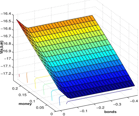
0 0.05 0.1 0.15 0.2 −0.4 −0.3 −0.2 −0.1 0 −17.2 −17.1 −17 −16.9 −16.8 −16.7 −16.6 −16.5 −16.4 bonds money V(e,b,m)
Figure 1: Value function as a function ofm and b.
household with a state (e, m) which is excluded from the credit market, Vd(e, m) is given by solving
Vd(e, m) = max
m′
u(cd(e, m)) +βEe′
(1−µ)W(e′,0, m′) +µVd(e′, m′)
where (1−µ) is the probability of coming back to the credit market in the next period with a level of unsecured debt b = 0. In this case, the value of not being excluded from the credit market is given by solving
W(e, b, m) = max
d∈{0,1}
max
b′,m′
u(cnd(e, b, m)) +βEe′W(b′, m′, e′) , Vd(e, m)
.
The household chooses to declare default, d(e, b, m) = 1, if
Vd(e, m)≥max
b′,m′
u(cnd(e, b, m)) +βEe′W(b′, m′, e′) .
Figure 1 shows W(e′, b′, m′) as a function of b and m.
Bankers
default decision of each individual,d(e, m, b), and the price of each bond,q(e, b, m;b′), according to their zero profit condition.
Government
The government is benevolent in the sense that its objective is to maximize the welfare of the consumers by choosing the level of inflation,πsubject to the budget constraint
M′− M
1 +π =T,
where M is the aggregate level of money balances such that M = P∞i=0mi and T
corresponds to aggregate collection of inflation tax. This inflation tax is rebated to the families. Therefore T =P∞i=0ζi.
2.1
Characterization of the demand for fiat money
An important result of this model consists in the fact that fiat money can be en-dogenously supported at equilibrium even when is dominated by the bonds in terms of its return. This subsection presents formally the intuition behind the household’s decision to demand fiat money.
In the current model economy, if a household defaults this household demands fiat money to smooth consumption by choosing m′ to solve:
−∂u(c
d(e, b, m))
∂cd +β
µE∂V
d(e′, m′)
∂m′ + (1−µ)E
∂W(e′,0, m′)
∂m′
= 0. (1)
Given that these households are not allowed to access the credit market, ∂Vd∂m(e,m) is, as in a Bewley (1980,1983) economy, strictly positive. If a household does not default, this household demands fiat money, m′, such that the following condition is satisfied:5
−∂u(c
nd(e, b, m))
∂cnd +βE
∂W(e′, b′, m′)
∂m′ = 0. (2)
In the other hand, while the decision regarding the unsecured bond, b′, is not a
5Figure 1 shows that W(e, b, m) is differentiable everywhere in m, then the second term in
equation (2) corresponds to:
E∂W(e
′, b′, m′)
∂m′ =
∂u(c′(e′, b′, m′))
∂c′
1 1 +π−
X
e′
(1−d(e′, b′, m′;b′′))∂q(e′, b′, m′;b′′)
∂m′ b
′′(e′, b′, m′)ν(e, e′) !
continuous one we can gain further intuition by thinking of it as being continuous for
the moment. Under that premise, the household would demand unsecured bonds b′
such that the following condition is satisfied:6
∂u(cnd(e, b, m)) ∂cnd
∂cnd(e, b, m) ∂b′ +βE
∂W(e′, b′, m′)
∂b′ = 0. (3)
Combining equations (2) and (3) we obtain that as the household finds it optimal to default with probability E[d(e′, b′, m′)]∈ (0,1), the following arbitrage condition holds:
1
1 +π −
X
e′
(1−d(e′, b′, m′))∂q(e
′, b′, m′;b′′)
∂m′ b
′′(e′, b′, m′)ν(e, e′)
=X
e′
(1−d(e′, b′, m′))
(
1
q(e, b, m;b′) + ∂q(e,b,m;b′)
∂b′ b′(e, b, m)
)
ν(e, e′) (4)
This arbitrage condition establishes that for positive default probabilities house-holds demand both money and bonds. The left hand side of the equation (4) corre-sponds to the marginal benefit of increasing the money holdings by one unit, while the right hand side corresponds to the opportunity cost of holding one unit of money. Increasing money holdings by one unit today allows households to consume 1+1π units tomorrow. Additionally increasing money holdings today increases bond prices tomor-row by ∂q(e′,b∂m′,m′′;b′′)b
′′(e′, b′, m′). On the other hand, increasing money holdings by one
unit today has a cost in terms of tomorrow’s consumption of 1
q(e,b,m;b′)+∂q(e,b,m;b′)
∂b′ b′(e,b,m) due to the forgone benefits of increasing bond holdings since increasing bond holdings also increases bond prices.
The arbitrage equation (4) holds with equality only for those agents that choose to demand money, i.e. agents having :
1>X e′
(1−d(e′, b′, m′))≥ 0.
6Figure 1 shows thatW(e, b, m) is not differentiable everywhere with respect tob. Ignoring such
issue for the moment we have that for equation (3) the derivative in the first term corresponds to
∂cnd
(e,b,m) ∂b′ =−
∂[q(e,b,m;b′)b′(e,b,m)]
∂b′ . The second term in equation (3)would be:
E∂W(e
′, b′, m′)
∂b′ =
∂u(c′(e′, b′, m′))
∂c′
X
e′
(1−d(e′, b′, m′;b′′))
1−∂q(e′, b′, m′;b′′)
∂b′ b
′′(e′, b′, m′)
ν(e, e′)
!
.
0 0.05 0.1 0.15 0.2
−0.4 −0.3 −0.2 −0.1 0
0 0.02 0.04 0.06 0.08 0.1 0.12
bonds money
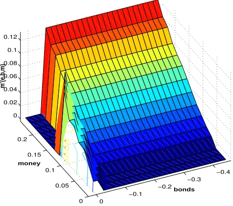
[image:11.612.188.426.40.250.2]m’(e,b,m)
Figure 2: Money Demand is a function of default probabilities.
All other agents do not demand money, unless the return on money is higher than the return on bonds, in which case they do not demand bonds. Figure 2 shows the money demand function for the region in which there are agents with probability 0 of default, positive probability of default, and probability 1 of default.
This corner solutions (either money or bonds are demanded) occur for households with
1 =X
e′
(1−d(e′, b′, m′)).
then q = 1+1r, so if inflation is higher than −r the return to bonds strictly dominate the return to money and the arbitrage equation has the form:
1 1 +π <
1
1 +r. (5)
it unimportant; the amount is even more important if we keep in mind that in the current context money is a very liquid asset given the assumption that it cannot be liquidated when households default on their debts.
2.2
Stationary Equilibrium
A steady-sate competitive equilibrium is a set of strictly positive prices,w∗,r∗, a non negative loan price vector, q(e, b, m;b′), an inflation rate, π∗, strictly positive quan-tities of aggregate labor,N∗, and capital, K∗, value functions W(e, b, m), Vd(e, m),
policy functions m′ = gm(e, b, m), b′ = gb(e, b, m), m′ = gd
m(e, m), d(e, b, m) and a
measure ϕ(e, b, m), such that the following conditions are satisfied:
1. Consumer’s optimization. Given the inflation rate,π∗, and the priceq(e, b, m;b′), the functions W(e, b, m), Vd(e, m) solve the consumer’s problem. The optimal policy functions are given by m′ = gm(e, b, m), b′ = gb(e, b, m), m′ = gd
m(e, m)
and d(e, b, m).
2. Competitive bankers make zero profits:
1
1 +r∗ =
X
e′
[1−d(e′, gb(e, b, m), gm(e, b, m))]q(e, b, m;gb(e, b, m)).
3. K∗ and N∗ solve the firms’ problem.
4. Labor market clearing:
N∗ = X
S
eϕ(e, b, m)
where S = [e, e]×b, b×[m, m].
5. Capital market clearing:
K∗ = X
S
[(1−d(e, b, m))q(e, b, m;gb(e, b, m))gb(e, b, m)]ϕ(e, b, m).
6. The stationary distributionϕ(e, b, m) is induced by exogenousν(e, e′) andgm(e, b, m).
gb(e, b, m), gd
m(e, m) and d(e, b, m) satisfy
ϕ(e, b, m) = X
S X
S′ 1{(g
b(e,b,m),(1−d(e,b,m))∗gm(e,b,m)+d(e,b,m)gmd(e,m))}ν(e, e
7. The inflation rate π satisfies
1 +π
π T =
X
S
(1−d(e, b, m))gm(e, b, m) +d(e, b, m)gmd(e, m)
ϕ(e, b, m).
2.3
Optimal Monetary Policy
The optimal monetary steady-sate competitive equilibrium for the model corresponds to an inflation rate ofπop whereπopis chosen by the government to maximize welfare
for the economy. We define the welfare of the economy as the expected discounted sum of utilities evaluated under the equilibrium stochastic consumption stream of an infinitely lived agent. The welfare function weights all agents equally.
Given that the government commitment problem is not the focus of this paper, we assume that the government has the technology to commit and chooses the same inflation rate in all periods. Given the complexity of the model, the optimal policy problem is solved numerically.
Despite the fact that the model has to be solved numerically, it is important to discuss the sources of the complexities in characterizing the optimal inflation rate. To begin with, inflation modifies the incentives to default by changing the return to money. A higher return to money implies it is less costly it is for the households to default. This result follows because holding money allows households to smooth consumption during periods of exclusion from credit markets; and more importantly money helps them to move part of their wealth from the period in which they default to the following periods of exclusion of credit markets. Therefore the higher is the return to money (the lower inflation is), the less costly it is to default, and therefore, other things equal, more default is observed.
More default (due to lower inflation) has a welfare cost because it implies less debt can be supported at equilibrium. That is, households face tighter credit constraints. This situation reduces the possibilities of households self insuring against a stream of negative income shocks through credit markets. On the other hand, more default (due to a lower inflation) has a welfare benefit because it is an alternative tool that allows the households to face a stream of negative income shocks. That is, default facilitates the non-contingent bonds to act as contingent bonds in some instances. In this way default helps to complete credit markets. Because of this effect, lower inflation is associated to a higher welfare in the economy.
if the transfers go from those with low endowment shocks to others agents in the economy, lower inflation would facilitate self insuring and therefore increase welfare in the economy.
In general, because the relation between inflation rates and welfare is non-monotonic and highly non-linear, the overall effect of inflation on welfare in this model cannot be predicted unambiguously without a quantitative analysis. Nevertheless, ignoring for the moment the fiscal effects of inflation, the opposing effects of default on welfare suggest that the optimal inflation rate should not be one that minimizes borrowing nor one that minimizes default. Since the Friedman rule inflation allows for very little borrowing and infinite inflation minimizes default, it is therefore possible to say that in general terms neither the Friedman rule inflation nor the infinite inflation correspond to the optimal monetary policy.
The following discussion further illustrates why the Friedman rule in not optimal in the current model. The Friedman rule policy minimizes borrowing because it gives the same return to money and bonds. Since money helps individuals to move resources from the period of default to periods of exclusion from credit markets, having a very high return to money makes the exclusion from credit markets almost painless. Under this scenario, Bulow and Rogoff (1987) show that it is impossible to support debt at equilibrium based purely on the reputation of the borrower. Under the Friedman rule policy, debt can be supported at equilibrium only if there are different punishments to default than the exclusion from credit markets.
3
Parametrization
The previously described model is computed for two different economies: the US, a developed economy with relative small idiosyncratic uncertainty and high enforcement of credit markets, and Colombia, a developing economy with relative high idiosyn-cratic uncertainty and low enforcement of credit markets. One period in the model is equivalent to a time period of a year. For both of these countries, the benchmark economy has an inflation rate of 0. This inflation rate is chosen for the benchmark because it allows a direct comparison of economies with different schemes of rebates of the inflation tax.
For both of these countries we assume that the endowment process follows a first-order autoregressive process for the natural logarithm of labor income: log(et) =
et+ρlog(et−1) +ξtwhereexit is i.i.d. normal with mean zero and standard deviation
σ. This process is simulated by a three-state Markov chain.
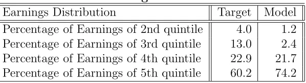
closely the parameterization of Chaterjee et al.(2006). The parameters are set to target the statistic on earnings obtained from the Survey of Consumer Finances of 2001 shown Table 1.
Table 1: U.S. Earnings Statistics SCF 2001
Earnings Distribution Target Model
Percentage of Earnings of 2nd quintile 4.0 1.2
Percentage of Earnings of 3rd quintile 13.0 2.4
Percentage of Earnings of 4th quintile 22.9 21.7
Percentage of Earnings of 5th quintile 60.2 74.2
The autocorrelation of the process is set to 0.75. In terms of matching the earnings process, a value of 0.32 for the variance of the shocks would be optimal, however, this value is too low to generate enough default at equilibrium. In Chaterjee et al. (2006), other shocks are used to fit this probability of default (e.g. preferences shocks and liability shocks), but to keep things simple and comparable with other models in the fiat money literature, we restrict ourselves to have only endowment shocks that represent labor income shocks. In order to generate enough default consistent with the observed one for the US, we increase the variance of the process to 0.4. While this value may seem high, it corresponds to the top of range of values considered in Aiyagari (1994).7
Regarding the production function and the utility function, the paper follows the guidelines of Aiyagari (1994). The capital share is set to 0.36 and the depreciation rate is 0.10. The risk aversion coefficient of the CRRA instantaneous utility function is 1.5 which is also used by Akyol (2004) and is consistent with the microeconomic estimates for the US economy. The discount factor is set to 0.95 which is a little bit smaller than the one of 0.96 used by Aiyagari but that is larger than those use by Chaterjee et al. (0.917) and Livshits et al. (0.94) to fit the default likelihood in the U.S. economy.
With respect to the exogenous probability of coming back to the markets, this probability is set to have an average period of exclusion from credit markets following a default of 10 years. 10 years is in line with the time that a bankruptcy in the US stays in an individual’s credit report. The punishment function for default is asymmetrical and is taken from the literature on sovereign default. The punishment is calibrated to fit the likelihood of default in the US economy and has the following
functional form:
φ(y) =
( b
y if y >yb y if y≤by
)
(6)
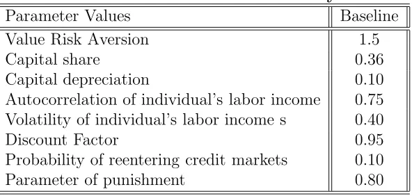
[image:16.612.143.439.155.296.2]A summary of the parameter values used in the simulation of the US economy is presented in Table 2.
Table 2: Parameters US Economy
Parameter Values Baseline
Value Risk Aversion 1.5
Capital share 0.36
Capital depreciation 0.10
Autocorrelation of individual’s labor income 0.75
Volatility of individual’s labor income s 0.40
Discount Factor 0.95
Probability of reentering credit markets 0.10
Parameter of punishment 0.80
For the Colombian economy, we use three of the same parameters that were used for the US economy: the coefficient of risk aversion, the discount factor, and the parameter for the punishment function for default.8
Regarding the stochastic process of the endowment, the values of the autocorre-lation coefficient and the variance of the shocks are chosen to replicate the inferred statistics of the distribution of the Colombian levels of income by quintile according to the report of the Colombian Department of Statistics (DANE) in its national Survey of Income and Expenses 1994−1995 found in Table 3.
Table 3: Colombia Income Statistics 1994-1995 (DANE)
Earnings Distribution Inferred Target
Percentage of Earnings of 2nd quintile 9.5
Percentage of Earnings of 3rd quintile 13.7
Percentage of Earnings of 4th quintile 20.9
Percentage of Earnings of 5th quintile 50.2
To replicate Colombia’s income distribution, the coefficient of autocorrelation is computed as the average of the autocorrelation of the participation in the total income
8Bonaldi et al. (2009) calibrate a quarterly discount rate of 0.9864 which is equivalent to annual
[image:16.612.138.444.496.579.2]of the 1st and 5th quintile of the income distribution for the years 1990−2001 reported by the Departmento de Planeacion Nacional (DPN) and shown in Table 4. The value for the coefficient of autocorrelation of the endowment process is then set to 0.865.
Table 4: Colombia 1st and 5th Income Quintile 1990-2001 (DPN)
Year 1st Quintile 5th Quintile
1990 4.8 54.1
1991 4.5 55.5
1992 4.4 56.4
1993 4.6 54.6
1994 4.2 56.9
1995 4.2 58.7
1996 4.1 57.2
1997 4.0 56.9
1998 3.7 59.8
1999 3.2 60.8
2000 3.0 61.7
2001 3.2 61.1
Given the value of the coefficient of autocorrelation of the endowment process, the value for the variance of the shocks that would match the model to the data in Table 3 would correspond to 0.37. However, as in the calibration for the US, since no other shocks that might be relevant to fit the default probability of the economy are considered, this parameter is chosen to fit the estimated probability of default. The value chosen is 0.415. Again, as in the case of the US calibration, this calibration strategy is comparable to previous models of heterogeneous agents and fiat money.
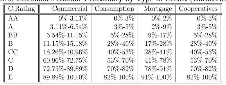
Table 5 shows the information on default probabilities reported by the bureau of credit in Colombia (Datacredito) for different types of credits and classified by the credit rating of the loan. Table 6 shows the information on the average relative proportion of total credits classified by their credit rating according to monthly data collected by the Agency of Supervision to the Financial System (Superintendencia Financiera SF) for the period December 2006 to January 2010.
Table 5: Colombia’s Default Probability by Type of Credit (Datacredito)
C.Rating Commercial Consumption Mortgage Cooperatives
AA 0%-3.11% 0%-3% 0%-2% 0%-3%
A 3.11%-6.54% 3%-5% 2%-9% 3%-5%
BB 6.54%-11.15% 5%-28% 9%-17% 5%-28%
B 11.15%-15.18% 28%-40% 17%-28% 28%-40%
CC 18.26%-40.96% 40%-53% 28%-41% 40%-53%
C 60.96%-72.75% 53%-70% 41%-78% 53%-70%
D 72.75%-89.89% 70%-82% 78%-91% 70%-82%
E 89.89%-100.0% 82%-100% 91%-100% 82%-100%
Table 6: Colombia’s Average proportion of Total Credit by Ratings (SF)
A B C D E
% 92.6 3.4 1.3 1.80 1.3
probability.
The share of physical capital in income is 0.37 which corresponds to the average share of physical capital for the period 1984−2005 as reported by Campo et al. (2008). The annual depreciation rate for Colombia is 0.115 and is taken from Bonaldi et al. (2009) which calibrate a quarterly depreciation rate for Colombia of 0.0287. The productivity parameter for Colombia is set to 0.64 following Parente and Prescott (1999); they estimate that since Colombia’s income was a 22% of the US’s income for the period 1950-88, then Colombia’s TFP should have been 64% of the US’s TFP.
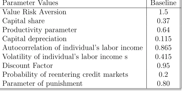
The exogenous probability of coming back to the markets after defaulting is 0.2. This value is consistent with an average exclusion from credit markets of 5 years; according to the Colombian law that created the bureau of credit, a bankruptcy stays in the credit report of an individual for 4 years. A summary of the parameter values used in the simulation of the Colombian economy is presented in Table 7.
3.0.1 Welfare
Table 7: Parameters Colombian Economy
Parameter Values Baseline
Value Risk Aversion 1.5
Capital share 0.37
Productivity parameter 0.64
Capital depreciation 0.115
Autocorrelation of individual’s labor income 0.865
Volatility of individual’s labor income s 0.415
Discount Factor 0.95
Probability of reentering credit markets 0.2
Parameter of punishment 0.80
level in the benchmark economy to measure welfare gains and losses in consumption units in percentage points.
3.0.2 Computation
The algorithm to compute the equilibria requires three steps: first, an inner loop where given the parameters and the prices (including the real interest rate), the individuals problem is solved; second, a middle loop where market clearing prices are obtained; and third an outside loop where the process is repeated for different levels of inflation. The individuals’ problem is solved using a simple value function iteration and interpolation methods. The equilibrium prices are found using Newton’s method. The grid for the bond position of the agents has 1275 points, and the grid for money balances has 15 points. Interpolation methods are used to find a solution that is continuous in money balances.
4
Results
We simulated the model in this paper for two different types of economies: developed economies with low degree of idiosyncratic uncertainty and high level of enforcement of debt contracts, and developing economies with high degree of idiosyncratic uncer-tainty and low level of enforcement of debt contracts.
en-dowment shocks and are proportional to the average demand for money of individuals with the same endowment shock. Both scenarios generate transfers of resources from the agents that hold money to other agents in the economy. However we call the first scenario the redistribution economy and the second one the non-redistribution economy because in the latter case there are no transfers between individuals with different endowment shocks; the transfers in this case are between individuals with the same endowment shock but different levels of debt.
The analysis of the redistribution economy allows us to focus on the welfare effects that monetary policy has through its impact on incentives to default. The compari-son of this economy to the non-redistribution economy allows us to focus on the fiscal effects that monetary policy has in the model. The comparison between the two different types of economies also allows us to focus on the role that the specific char-acteristics of the economies (i.e. the volatility and persistence of idiosyncratic shocks as well as the degree of enforcement of credit contracts) has in the determination of the optimal monetary policy.
4.1
Welfare and Real Implications of Optimal Monetary
Pol-icy
In this sub-section we focus on the redistribution economy, that is the economy in which the government transfers the inflation tax back to the individuals proportionally to the average demand for money. We ignore more sophisticated fiscal policies, and assume that the government cannot or does not want to incentive insurance through the implementation of specific, targeted schemes of transfers.
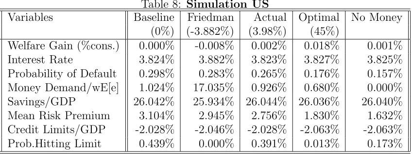
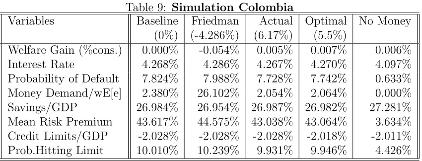
[image:20.612.77.502.492.651.2]The results of this analysis for the US are presented in Table 8 and Table 10; the results for Colombia are presented in Table 9 and Table 11.
Table 8: Simulation US
Variables Baseline Friedman Actual Optimal No Money
(0%) (-3.882%) (3.98%) (45%)
Welfare Gain (%cons.) 0.000% -0.008% 0.002% 0.018% 0.001%
Interest Rate 3.824% 3.882% 3.823% 3.827% 3.825%
Probability of Default 0.298% 0.283% 0.265% 0.176% 0.157%
Money Demand/wE[e] 1.024% 17.035% 0.926% 0.680% 0.000%
Savings/GDP 26.042% 25.934% 26.044% 26.036% 26.040%
Mean Risk Premium 3.104% 2.945% 2.756% 1.830% 1.632%
Credit Limits/GDP -2.028% -2.046% -2.028% -2.063% -2.063%
Table 9: Simulation Colombia
Variables Baseline Friedman Actual Optimal No Money
(0%) (-4.286%) (6.17%) (5.5%)
Welfare Gain (%cons.) 0.000% -0.054% 0.005% 0.007% 0.006%
Interest Rate 4.268% 4.286% 4.267% 4.270% 4.097%
Probability of Default 7.824% 7.988% 7.728% 7.742% 0.633%
Money Demand/wE[e] 2.380% 26.102% 2.054% 2.064% 0.000%
Savings/GDP 26.984% 26.954% 26.987% 26.982% 27.281%
Mean Risk Premium 43.617% 44.575% 43.038% 43.064% 3.634%
Credit Limits/GDP -2.028% -2.028% -2.028% -2.018% -2.011%
[image:21.612.96.480.279.357.2]Prob.Hitting Limit 10.010% 10.239% 9.931% 9.946% 4.426%
Table 10: Optimal Inflation and Inflation Costs by Income US
Optimal Inflation Inflation Costs/Gains
Whole Economy 45.0% 0.0028%
Low endowment shocks 50.0% 0.0050%
Medium endowment shocks 45.0% 0.0020%
[image:21.612.93.483.437.513.2]High endowment shocks 16.0% 0.0073%
Table 11: Optimal Inflation and Inflation Costs by Income Colombia
Optimal Inflation Inflation Costs/Gains
Whole Economy 5.5% 0.0094%
Low endowment shocks 6.5% 0.0076%
Medium endowment shocks -3.0% 0.0030%
High endowment shocks 85.0% 0.0114%
Tables 8, 9, 10 and 11 summarize the numerical findings. We summarize the results of this experiments as follows:
1. The model replicates several of the observed facts of the two economies.
corresponds to the average inflation rate for the US from 1946 to 2001, the de-fault rate predicted by the model is 0.27%; the actual value of this probability is 0.30%, only 0.03% more than the value predicted by the model. For Colom-bia, with an annual inflation rate of 6.17%, which corresponds to the average inflation rate for Colombia from 2000 through 2010, the default rate predicted by the model is 7.72%, which is in the range of 4.8% to 8.7% computed for this statistic in based on the available data.
For the US, the interest rate predicted by the model for the actual inflation rate of this economy, 3.9%, corresponds to 3.82%. This value does not differ too much from the level of 4.06% observed for the annualized interest rates in 3 months T-Bills in this economy. Given the average risk premium of 2.76% predicted by the model for the actual level of inflation, the average interest rate on unsecured debts predicted by the model is around 6.58%. Based on the period 2005−2009, this value is lower than the actual values for the average APR in new credit cards (11.86%) or 24-months personal loans (12.06%), but it is not that far from the average interest rate on 48-months new car loans (7.39%).
For Colombia, the interest rate predicted by the model for the actual inflation rate of this economy, 6.17%, corresponds to 4.27%. This value is lower than the level of 10.0% observed for new public debt in this economy for the period 2005-2010. However, as should be expected, the average interest rate for Colombia is larger than the one for the US.
Given the average risk premium predicted by the model for the actual Colom-bian level of inflation, the average interest rate on unsecured debts is 47.31%. Looking again to the period 2005−2009, this rate is too high in comparison to both the average APR for credit cards of 26.82%, or the average interest rate on consumption loans for the same period of 23.19%. However this difference between the predicted interest loan rate and the actual one is smaller than the one predicted by other models of heterogeneous agents where individuals default on their debts. 9
Also, as in the data, the percentage of investment-to-GDP is similar in both types of economies, but the actual GDP of the developing economy is much smaller than the one of the developed economy. In the model, Colombia’s GDP is 56.07% of the US’s GDP. This is much higher than the 22.0% for Colombia’s
9For example the model of Chatterjee et al.(2006) predicts for the US an average loan interest
GDP in comparison to US’s GDP reported by Parente and Prescott (1999), but the result is consistent in qualitative terms.
2. In the model, individuals hold both bonds and fiat money.
While the amount of wealth that the agents hold in money balances is not very large, households in both economies keep part of their wealth in money. Consis-tent with the notion that poorer individuals hold a larger part of their wealth in money balances, the households in the developing economy hold (proportionally to their labor income, wEe) a larger amount of money than the households in the developed economy. For example for the actual levels of inflation in each economy we have that in the US the average money demand corresponds to 0.926% of the households’ labor income while in Colombia the average money demand corresponds to 2.054% of the households’ labor income.
3. Allowing individuals to hold money increases the probability of default.
This increase in the probability of default is much larger for the developing economy than for the developed economy: comparing the economy without money to the economies with money in which the inflation rate is equivalent to the average observed inflation rate in each of the economies, the probability of default increases by a factor of 11.5 for the developing economy and only by a factor of 1.7 for the developed economy.
Furthermore, for the developing economy the relation between inflation rate and default probability is an inverse one: higher inflation rate implies lower default probability. On the other hand, for the developed economy the relation is non-monotonic. For negative values of inflation, higher inflation implies higher probabilities of default while for positive levels of inflation, higher inflation rates imply lower probabilities of default.
The relation between negative values of inflation and default probability in the developed economy illustrates that when inflation is very low and therefore the punishment for default is relatively soft, there is less debt at equilibrium, and therefore less default.
4. Allowing individuals to hold money has the potential to increase welfare in the economy.
rate is the optimal inflation rate in each of them, welfare increases by 0.001% for the developing economy and by 0.017% for the developed economy.
While these gains are small quantitatively, they are potentially important. For example, looking at the US case, allowing individuals to hold money generates a welfare gain that is 12 times the welfare gain of eliminating business cycles in the US economy as calculated by Lucas (1987).
5. The Friedman rule is not in general the optimal monetary policy in this model.
For the economies studied here, the optimal monetary policy is one that implies a positive inflation rate. It should be noted that the optimal monetary policy differs across economies: First, the optimal annual inflation rate is larger for the more developed economy. For the US the optimal inflation rate corresponds to 45.0% annually compared to 5.5% annually for Colombia; second, the welfare gains of departing from the Friedman rule are larger for the developing economy (0.0607%) than for the developed one (0.0258%).10
Additionally, in both economies individuals would be better off by not having money at all than by following the Friedman rule. The obvious intuition for such result is that the Friedman rule inflation rate generates too little borrowing and too much default.
As discussed previously, inflation has an important role in affecting the incen-tives to default. Optimal inflation is positive, between two alternative logical extremes, i.e. the Friedman rule for the lower limit and infinite inflation for the higher limit. This result implies that the optimal level of default is neither the maximum possible (for inflations near to the Friedman rule) nor the minimum one (for infinite inflation). In practical terms, this result highlights the role that default might have in enhancing the efficiency of the allocations in the economy. That is, the optimal inflation rate highlights that some degree of default might be desirable.
Finally, since higher inflation rates make the punishment for default stronger, the result for optimal inflation implies that for the developed economy the benefits of default are smaller than for the developing economy. Therefore, it can be concluded that default is more useful as a means to enhance the efficiency of the allocations for those economies that face higher degree of uncertainty.
10For the US economy, the welfare loss of following the Friedman rule in the current model is
Regarding the results for the optimal inflation rate for the United States, which looks too high, it is worth mentioning that by looking at money only as a medium to store wealth and ignoring the transactional role of money in the economy, we may underestimate the inflation costs in the economy. Surely modeling the transactional role of money would produce a more reasonable estimate. Instead, the current paper focuses on the qualitative message of the current model. That is, in addition to its more obvious effects, monetary policy can also influence welfare through its effect on the incentives to default. Ignoring the other functions of money helps us to focus completely on this new aspect of monetary policy that has previously been overlooked.
6. In both economies, the optimal inflation rate varies according to the endowment shock.
For the developed economy, the optimal inflation rate for those with the low endowment shocks is 50%, while the optimal inflation rate for those with the medium endowment shocks is 45%, and the optimal inflation rate for those with high endowment shocks is 16%.
For the developing economy, the optimal inflation rate for those with low en-dowment shocks is 6.5%, while the optimal inflation rate for those with the
medium endowment shocks is −3%, and the optimal inflation rate for those
with high endowment shocks is 85%.
These results suggest that in the developed economy individuals with high en-dowments potentially value the option to default more than individuals with low endowments, even when, in general, these individuals are less likely to de-fault. This conclusion holds because individuals with high endowments do not demand money. Therefore they benefit the most from transfers due to high in-flation rates; their preference for relatively low inin-flation rates is signaling than they heavily weigh the benefits of a low inflation, which reduce the welfare costs of default.
For the developing economy, the picture is quite different since in this case those that value more the option to default are the ones with low and medium income shocks. This result can be interpreted to imply that these individuals are using default as a mean to insure themselves against very low consumption streams.
7. The average costs/gains of inflation in this model, while small, are dependent on the type of the economy and on the level of inflation.11
The average cost/gain of a change of one percent in inflation for the US (0.0028%) is a third of the average cost/gain for Colombia (0.0094%). While these costs are smaller than those found for the US by Kehoe et al (1992) for the US (0.004%), these costs/gains are highly dependent on the level of inflation. For example, for the US, reducing the inflation rate from −3% by one percent (to-wards the inflation rate consistent with the Friedman rule) generates a welfare loss in terms of consumption of 0.0061%. This loss corresponds to 2.2 times the average cost/gain from changing inflation by one percent in this economy. For Colombia, reducing the inflation rate from−3.5% by one percent (towards the inflation rate consistent with the Friedman rule) generates a welfare loss in terms of consumption of 0.0428%. This loss corresponds to 4.6 times the average cost/gain from changing inflation by one percent in this economy.
8. The average costs/gains of inflation in this model are dependent on the endow-ment shock.
For the US, as previously mentioned, the average cost/gain of a change of one percent in inflation is 0.0028%. However for individuals with a low endow-ment shock this average cost/gain is 0.005%, while for the individuals with the medium income shock the average cost/gain is 0.002%, and for the individuals with high endowment shock this average cost/gain is 0.0073%. For Colombia, the average cost/gain of a change of one percent in inflation is 0.0094%. However for individuals with a low endowment shock this average cost/gain is 0.0076%, for the individuals with medium income shock the average cost/gain is 0.003%, and for the individuals with high endowment shock this average cost/gain is 0.0114%.
The pattern is the same for both economies: the individuals at the extremes of the income distribution (compared to those in the middle) are those that have potentially more to gain or lose from changes in inflation.
The effects of inflation changes on welfare gains/losses differs strongly across individuals and economies. For example, in Colombia, individuals with high endowment like high inflation due to strong punishment for default and high transfers across individuals. On the other hand, in the US, individuals with high endowments like low inflation due to soft punishment for default and low transfers across individuals. In both Colombia and the US, individuals with low endowment like high inflation in comparison to the absolute optimal inflation
rate due to strong punishment for default and high transfers. Finally, in Colom-bia, individuals with the medium income shock like very low inflation while in the US these individuals like to have the average optimal inflation rate which corresponds to the high level of inflation of 45.0%.
These results can be explained by an important difference between the US and Colombia: in the US only the individuals with a low endowment shock default on their debts. Instead in Colombia both individuals with low and medium endow-ment shock default on their debts. Therefore, while in Colombia any transfers that occur between individuals go only to the high endowment individuals, in the US these transfers are shared by both medium and high endowment indi-viduals. As a result, the incentive in Colombia for the individuals with high endowment to prefer high inflation is much stronger. On the other hand, in the US, looking at the individuals with high endowment and medium endowment shocks, the former are the less concerned with tight credit limits. Therefore they are capable of tolerating high inflation.
Regarding the behavior of individuals with low endowments, we can observe that for these individuals tight credit limits are a problem. Therefore they might prefer a high inflation that penalizes default in a harsher way, since defaulting on a very low level of debt might not be enough to protect them from a series of low endowments shocks.
Finally, the behavior of the individuals with medium endowment shocks is dif-ferent in the two countries because individuals with medium endowment shocks in Colombia benefit from being able to borrow somewhat more than the individ-uals with low endowment shocks and can therefore use default more efficiently to smooth their consumption.
9. Inflation has real effects in the model.
For the US, an increase of one percent in inflation generates an average change in aggregate production of 1.1433%, and an average change in aggregate capital of 0.8257%.
For Colombia, an increase of one percent in inflation generates an average change in aggregate production of 0.3001%, and an average change in aggregate capital of 0.1753%.
impact of inflation on aggregate savings for the developed economy than the developing economy.
Importantly, in the current model the relation between inflation an capital ac-cumulation for the US is hump-shaped as is the one observed in the data. Ad-ditionally, in line with the empirical study of Bullard and Keating (1995) that finds that the level of the inflation rate that maximizes capital accumulation for the US is in the range between 3% and 6%, the annual level of inflation that maximizes capital accumulation for the US in here corresponds to 5.5%.
As opposed to the US, for Colombia the relation between the inflation rate and capital accumulation is monotonically increasing, i.e. more inflation equals more capital accumulation. This result implies that when default increases precautionary savings also increase.
For the case of Colombia, one possible explanation for the relation between inflation and capital accumulation is as follows: there is a negative effect in risk sharing of the transfers that occur between the agents in the economy that hold money and the agents that do not hold money. This effect is so strong that in order to outweigh this impact of the transfers, it is necessary for the agents to both default more and hold more precautionary savings.
Two possible issues arise regarding the treatment of Colombia in the model. First, Colombia faces a relatively large aggregate uncertainty, and taking into account this issue could potentially modify the results. This issue is a question for further research. Second, Colombia is not a closed economy, as modeled in the paper, but instead a small open economy, and therefore takes the interest rate as given. This issue does not appear to affect the results: recomputing the model taking the interest rate as given, the annual optimal level of inflation is around 5.2%; the corresponding default probability for the economy is 9.3%; and welfare is relatively low when the economy follows the Friedman rule, which is associated to a much larger default probability.
4.2
Fiscal Effects of Monetary Policy
The results of this analysis for the US are presented in Table 12; the results for Colombia are presented in Table 13.
Table 12: Simulation US
Variables Baseline Friedman Actual Optimal No Money
(0%) (-3.914%) (3.98%) (40%)
Welfare Gain (%cons.) 0.000% 0.010% 0.002% 0.011% 0.001%
Interest Rate 3.824% 3.914% 3.820% 3.914% 3.825%
Probability of Default 0.298% 0.295% 0.265% 0.172% 0.157%
Money Demand/wE[e] 1.024% 17.047% 0.929% 0.692% 0.000%
Savings/GDP 26.042% 25.874% 26.050% 26.062% 26.040%
Mean Risk Premium 3.104% 3.071% 2.757% 1.770% 1.632%
Credit Limits/GDP -2.028% -2.046% -2.028% -2.063% -2.063%
[image:29.612.72.507.296.453.2]Prob.Hitting Limit 0.439% 0.000% 0.391% 0.013% 0.173%
Table 13: Simulation Colombia
Variables Baseline Friedman Actual Optimal No Money
(0%) (-4.347%) (6.17%) (Friedman)
Welfare Gain (%cons.) 0.000% 0.025% -0.002% 0.025% 0.006%
Interest Rate 4.268% 4.347% 4.264% 4.347% 4.097%
Probability of Default 7.824% 8.865% 7.686% 8.865% 0.633%
Money Demand/wE[e] 2.380% 25.975% 2.044% 25.975% 0.000%
Savings/GDP 26.984% 26.851% 26.992% 26.851% 27.281%
Mean Risk Premium 43.617% 50.056% 42.752% 50.056% 3.634%
Credit Limits/GDP -2.028% -2.028% -2.028% -2.028% -2.011%
Prob.Hitting Limit 10.010% 11.160% 9.891% 11.160% 4.426%
Tables 12 and 13 summarize the numerical findings in this sub-section. We summarize the results of this experiment as follows:
1. In both economies, eliminating transfers across individuals with different en-dowment shocks reduces the optimal rate of inflation.
This result is counter intuitive. Since a cost of inflation is being taken away by eliminating transfers across agents with different endowments, it should be easier to observe higher inflation rates in the economy. The result is poten-tially more confusing, if we look in detail to what occurs in both economies, For example, for the US, looking at the economy that follows the optimal in-flation rate, under this scenario all individuals are saving more than when the
transfers occur—low endowment individuals save a 0.25% more, medium
en-dowment individuals save a 0.22% more, and high endowment individuals save a 0.08% more). At the same time, the probability of default falls by 2.57%. For Colombia, looking at the economy that follows the optimal inflation rate, under this scenario some individuals are saving more and others less than when the transfers occur—low endowment individuals save 0.70% more, medium en-dowment individuals save a 1.55% less, and high endowment individuals save 0.30% less. At the same time, the probability of default increase by 6.8% for low endowment individuals and by 16.4% for high endowment individuals.
The explanation of these potentially confusing results depends on the particulars of each economy. For the US, when the transfers across individuals with different endowment shocks are eliminated, the usage of default as a mean of enhancing the allocations of the market is less necessary. In this case, pure simple savings work better. That is, for the US, default is only used as a last resource, and it is better avoided when possible. So for the US, eliminating transfers across individuals with different endowments reduces the problems of risk sharing in the economy. This reduction makes the usage of default less desirable.
For Colombia the opposite seems to hold true. When the transfers are elimi-nated, more default and less savings are observed. In order to have more default a lower inflation rate is necessary. For Colombia, default is a tool that is used as actively as possible to enhance the allocations of the financial markets.
This analysis implies that for economies with low idiosyncratic uncertainty, default should be avoided when possible, while for economies with high degree of idiosyncratic uncertainty default should be used as much as possible. For the latter economies, default helps to improve the allocations that could be obtained only through the use of incomplete credit markets.
2. In both economies, the optimal inflation rate varies according to the endowment shock.
inflation rate for those with the medium endowment shocks is 45%, and the optimal inflation rate for those with high endowment shocks is 8.5% (vs 16% with transfers). Comparing these rates to the observed ones when transfers occur, we find that for both individuals with low and high endowment shocks, the preferred inflation rate is much lower without transfers than with transfers. For individuals with medium endowment shocks, the rate is unchanged. With-out transfers, the individuals at the extremes of the income distribution (low and high) would like a softer punishment for default. These preferences reveal stronger incentives to default. These incentives result in an equilibrium effect where credit tightens and less default is observed.
For the developing economy, we observe that the optimal inflation rate for those with low endowment shocks is−4.35% (vs 6.5% with transfers), the optimal in-flation rate for those with the medium endowment shocks is also −4.35%(vs
−3% with transfers), and the optimal inflation rate for those with high endow-ment shocks is 90% (vs 85% with transfers). In this case, the individuals that default at equilibrium (low and medium endowment) prefer a very low inflation rate, so that the punishment for default is comparatively soft. In the other extreme, the individuals that never default (high endowment) prefer a much harsher punishment for default because now they do not benefit from transfers. Therefore they rely even more on the functioning of credit markets to smooth their consumption. At the same time the high persistence of the endowment process implies less benefits for them from the option of default.
3. The average costs/gains of inflation in this model change when no transfers across individuals with different endowment shocks occur.
For the US, the average cost/gain of a change of one percent in inflation is twice as large in the non-transfer scenario (0.0061% vs. 0.0028% with transfers). For Colombia, the average cost/gain of a change of one percent in inflation falls by a third (0.0067% vs. 0.0094% with transfers).
It is worth noting that without transfers across individuals with different endow-ment shocks, the average welfare cost/gain of a one percent change in inflation is roughly the same for both types of economies. Therefore it is clear that the welfare effects of inflation are highly dependent on the fiscal policy that the economy follows.
increases for all individuals;12 instead for Colombia this average cost/gain falls for individuals with low endowment shocks, stays the same for the individu-als with medium endowment shocks, and increases for individuindividu-als with high endowment shocks.13
The pattern for the individuals with high endowment shocks stays the same as before: in both economies the individuals that face a higher average welfare cost/gain when inflation changes in one percent are those with high endowments. In relation to the scenario with transfers, these average costs/gains are larger because individuals with high endowment shocks do not benefit anymore from the transfers.
Regarding the pattern for individuals with low and medium endowment shocks there is a change: without transfers both types of individuals are roughly equally affected by changes in the inflation; in contrast, with transfers the individuals with low endowment shocks face stronger welfare effects of inflation. The result is obvious since now individuals with low endowment shocks are not transferring resources to other agents in the economy.
A slightly counterintuitive result is the increase in the size of the effects of inflation in the individuals of low and medium endowment shocks in the US. One possible explanation is that in absence of transfers, these types of individuals have more resources available that in principle would allow them to smooth consumption even better in the absence of access to credit markets. This effect generates stronger incentives to default. In turn, stronger incentives to default at any inflation rate modify the response of welfare to changes in the punishment to default via changes in the inflation rate.
4. Real effects of inflation are stronger than in the model with transfers.
For the US, an increase of one percent in inflation generates an average change in aggregate production of 1.6854%, and an average change in aggregate capital of 1.2095%.
12In the US, for the individuals with low endowment shocks, a one percent change in inflation
im-plies that the average welfare cost/gain goes from 0.005% with transfers to 0.006% without transfers; for the individuals with medium endowment shocks it goes from 0.002% with transfers to 0.005% without transfers; and for the individuals with high endowment shocks it goes from 0.007% with transfers to 0.0140% without transfers
13In Colombia, for the individuals with low endowment shocks, a one percent change in
For Colombia, an increase of one percent in inflation generates an average change in aggregate production of 0.7463%, and an average change in aggregate capital of 0.4670%.
The magnitude of the effects is larger for both economies than in the economies with transfers across individuals with different endowment shocks, implying a stronger effect of inflation in aggregate savings in the absences of transfers.
5
Conclusions
In this paper we extend the literature of heterogeneous agent models that face id-iosyncratic earnings shocks and incomplete credit markets. We introduce endogenous default and fiat money that cannot be liquidated to pay off unsecured debts. This framework allows us to study the implications of limited commitment on the side of the debtors. We uncover four main effects: first, fiat money supported at equilibrium; second, the determination of the optimal monetary policy for the economy; third, the role that default might have in improving the efficiency of equilibrium allocations; and fourth, the effects of inflationary tax policies in the degree of risk sharing of the economy.
In studying incomplete credit markets, when we consider not only bonds but also other very liquid assets that cannot be liquidated in the case of default (fiat money), we find that it is easier to replicate the default rates observed in the data than when the only asset is bonds.
When we consider that the alternative asset to bonds is fiat money, then monetary policy can have powerful effects in the incidence of default in the economy. Very expansionary monetary policies that imply high levels of inflation strengthen the punishment for default. Therefore these policies reduce the likelihood of observing default and increase the amount of debt that is observed at equilibrium. On the contrary, very restrictive monetary policies make the punishment for default soft. Therefore these policies increase the likelihood of default at equilibrium and tighten credit limits.
Interestingly, avoiding default is not necessary the best policy in this context. Default is an option that the households can use to insure themselves against streams of low endowment shocks instead of accumulating too many precautionary savings. As a consequence, the optimal inflation rates varies from economy to economy, because the optimal level of default also varies.
of the credit market allocations. Because default is more useful for the economy with a high degree of idiosyncratic uncertainty, the optimal inflation for this economy is lower than for the economy with a low degree of idiosyncratic uncertainty. That is, in order to have a sufficient occurrence of default in the economy with a high degree of uncertainty, the inflation rate needs to be low enough such that the punishment for default is not too harsh. In contrast, the economy with a low degree of uncertainty needs a harsher punishment of default and therefore a higher inflation rate.
In the current model the Friedman rule might be, but is not in general, the optimal policy. The inflation consistent with the Friedman rule is such that the return to bonds and money are equal. This parity allows households to default and thereby transfer the resources that they did not use to pay their debt in order to smooth their future consumption in a very efficient way. Therefore, following the Friedman rule implies a very high likelihood of default and the impossibility of supporting borrowing at equilibrium using only punishments based on the reputation of the households. The Friedman rule then implies very tight credit limits for the economy.
Regarding the levels of the optimal inflation rates, while the quantitative results of the model might seem too high, at least for the US, the results highlight the importance of taking in account the return to money. Specifically, changing the return to money affects the likelihood of default in the economy. This is an important effect that is not considered by policy makers but that should not be disregarded when formulating the monetary policy for the economy.