Multimodal Estimation of Distribution Algorithms
Qiang Yang, Student Member, IEEE, Wei-Neng Chen, Member, IEEE, Yun Li, Member, IEEE,
C. L. Philip Chen, Fellow, IEEE, Xiang-Min Xu, Member, IEEE,
and Jun Zhang, Senior Member, IEEE
Abstract—Taking the advantage of estimation of distribution algorithms (EDAs) in preserving high diversity, this paper pro-poses a multimodal EDA. Integrated with clustering strategies for crowding and speciation, two versions of this algorithm are developed, which operate at the niche level. Then these two algorithms are equipped with three distinctive techniques: 1) a dynamic cluster sizing strategy; 2) an alternative utiliza-tion of Gaussian and Cauchy distribuutiliza-tions to generate offspring; and 3) an adaptive local search. The dynamic cluster sizing affords a potential balance between exploration and exploita-tion and reduces the sensitivity to the cluster size in the niching methods. Taking advantages of Gaussian and Cauchy distri-butions, we generate the offspring at the niche level through alternatively using these two distributions. Such utilization can also potentially offer a balance between exploration and exploita-tion. Further, solution accuracy is enhanced through a new local search scheme probabilistically conducted around seeds of niches with probabilities determined self-adaptively accord-ing to fitness values of these seeds. Extensive experiments
Manuscript received August 29, 2015; revised November 24, 2015; accepted January 21, 2016. This work was supported in part by the National Natural Science Foundation of China Project under Grant 61379061, Grant 61332002, and Grant 61511130078, in part by the Natural Science Foundation of Guangdong for Distinguished Young Scholars under Grant 2015A030306024, in part by the Guangdong Special Support Program under Grant 2014TQ01X550, and in part by the Guangzhou Pearl River New Star of Science and Technology Project under Grant 201506010002. This paper was recommended by Associate Editor P. P. Angelov. (Corresponding author: Wei-Neng Chen.)
Q. Yang is with the Key Laboratory of Machine Intelligence and Advanced Computing, Ministry of Education, Guangzhou 510006, China, also with the Engineering Research Center of Supercomputing Engineering Software, Ministry of Education, Guangzhou 510006, China, and also with the School of Data and Computer Science, Sun Yat-sen University, Guangzhou 510006, China.
W.-N. Chen is with School of Computer Science and Engineering, South China University of Technology, Guangzhou, 510006, China, also with the Key Laboratory of Machine Intelligence and Advanced Computing, Ministry of Education, Guangzhou, 510006, China, and with the Engineering Research Center of Supercomputing Engineering Software, Ministry of Education, Guangzhou, 510006, China (e-mail:[email protected]).
Y. Li is with the School of Engineering, University of Glasgow, Glasgow G12 8LT, U.K.
C. L. P. Chen is with the Department of Computer and Information Science, University of Macau, Macau 999078, China.
X.-M. Xu is with the School of Electronic and Information Engineering, South China University of Technology, Guangzhou 510006, China.
J. Zhang is with the Key Laboratory of Machine Intelligence and Advanced Computing, Ministry of Education, Guangzhou 510006, China, and also with the Engineering Research Center of Supercomputing Engineering Software, Ministry of Education, Guangzhou 510006, China (e-mail:
This paper has supplementary downloadable multimedia material available athttp://ieeexplore.ieee.orgprovided by the authors. This includes a PDF file that contains additional tables not included within the paper itself. The total size of the file is 1.17 MB.
Color versions of one or more of the figures in this paper are available online athttp://ieeexplore.ieee.org.
Digital Object Identifier 10.1109/TCYB.2016.2523000
conducted on 20 benchmark multimodal problems confirm that both algorithms can achieve competitive performance compared with several state-of-the-art multimodal algorithms, which is supported by nonparametric tests. Especially, the proposed algo-rithms are very promising for complex problems with many local optima.
Index Terms—Estimation of distribution algorithm (EDA), multimodal optimization, multiple global optima, niching.
I. INTRODUCTION
M
ULTIMODAL optimization, which seeks multiple optima simultaneously, has received much atten-tion recently. Many real-world problems involve mul-tiple optima, such as protein structure prediction [1], holographic design [2], data mining [3]–[5], and electro-magnetic design [6], [7]. Hence, it is desirable to find as many optima as possible in the global optimization. However, different from finding just one optimum in sin-gle optimization [8]–[13], locating multiple global or local optima simultaneously is qualitatively more challenging.For such problems, classical evolutionary algorithms (EAs), including differential evolution (DE) [9], [14]–[19], genetic algorithm (GA) [20], [21], and particle swarm optimiza-tion (PSO) [12], [22]–[25], lose feasibility and effectiveness, because their overall learning and updating makes the pop-ulation tend to converge toward one dominating candidate. Therefore, to locate multiple optima simultaneously using clas-sical EAs, a multimodality-specific mechanism is necessary.
So far, niching [26]–[29] has been widely used to help an EA maintain a diverse population in multimodal opti-mization. Niching achieves this by partitioning the whole population into subpopulations using techniques such as crowding [29] and speciation [30]–[32] and each subpopula-tion is responsible for one area to locate one or a small number of optima. Because of the sensitivity to parameters in niching methods, for instance, crowding [29] is sensi-tive to the crowding size and speciation is sensisensi-tive to the niching radius [30], [31], various free or parameter-insensitive techniques are hence developed to improve niching, such as hill-valley [32]–[34], recursive middling [35], history-based topological speciation [36], and clustering [37], [38]. However, these niching techniques either cost a number of fit-ness evaluations or require a large memory or introduce less sensitive parameters to partition the population into niches.
Alternative to niching, learning, and updating strate-gies are modified to enhance the diversity for EAs, such as GA [26], [28], [35], DE [38]–[40], and PSO [41], [42].
The resultant algorithms extend learning beyond domi-nant individuals by offering relatively poor individuals improved survival to the next generation [38]–[40]. Together, they maintain the diversity of the population at the individual level.
Recently, a new family of EAs—the estimation of distribution algorithms (EDAs) [10], [11], [43]–[46] has emerged, which preserves diversity at the population level. Generally, an EDA generates offspring by sampling from the probability distribution estimated from promising indi-viduals. However, current EDAs are designed for sin-gle optimization and so far, there exists no report in the literature on applying EDAs to deal with multimodal optimization.
Since an EDA maintains significant diversity at the popu-lation level, it should offer improved assistance for locating multiple optima. Motivated by this observation, we propose a multimodal EDA (MEDA), to cope with multimodal opti-mization. Specifically, the characteristics of MEDA are as follows.
1) Two popular niching strategies, crowding and specia-tion, are incorporated in MEDA, leading to MCEDA and MSEDA, respectively. Instead of operating at the population level, MEDAs (MCEDA and MSEDA) oper-ate at the niche level. Further, different from traditional EDAs, all individuals in every niche participate in the estimation of distribution of that niche.
2) A dynamic cluster sizing strategy is proposed to coop-erate with the two niching methods. This strategy not only affords a potential balance between exploration and exploitation, but also reduces the sensitivity of the used niching methods to the cluster size.
3) Gaussian distribution and Cauchy distribution are alter-natively used to generate offspring for each niche, instead of just using Gaussian distribution in classi-cal EDAs. Taking the advantages of both distributions, this alternative usage offers an extra potential balance between exploration and exploitation.
4) A new local search scheme based on Gaussian dis-tribution is proposed to refine the obtained solutions, leading to local search-based MEDAs (LMEDAs), con-taining LMCEDA and LMSEDA. This local search is probabilistically performed around seeds of niches with probabilities self-determined according to fitness values of these seeds.
Extensive experiments have been conducted on 20 widely used benchmark multimodal functions and the experimental results supported by nonparametric Wilcoxon rank-sum test consistently demonstrate that LMEDAs are able to provide better and more consistent performance than the state-of-the-art multimodal algorithms on majority of the bench-mark functions without incurring any serious computational burden.
Following a review of multimodal optimization techniques and EDAs in Section II, the proposed MEDAs are detailed in Section III. Extensive experiments are conducted to test MEDAs in Section IV. Finally, the conclusions and discussions are presented in Section V.
Algorithm 1 Crowding-Based DE (CDE) [29]
Input: population size NP, crowding size K
1: Randomly initialize the population; 2: For i=1 to NP
3: Produce a child oi using standard DE;
4: Randomly select K individuals in the population to form a crowd;
5: Compare the fitness of oi with that of the nearest individual found by Eq. (1) and replace it if oi is better;
6: End For
7: Stop if the termination criterion is met. Otherwise go to Step 2;
Output: the whole population
II. MULTIMODALOPTIMIZATION ANDESTIMATION OFDISTRIBUTIONALGORITHMS
Without loss of generality, maximization multi-modal problems are considered in this paper as in [26], [29], [30], [32], [36], [37], [39]–[42], and [47]–[49]. In addition, in the literature, locating multiple global optima is the main objective of multimodal optimization, and hence is also the concern of this paper.
A. Multimodal Optimization Algorithms
Generally, to cope with multimodal optimization effi-ciently, two major issues need to be addressed: 1) diver-sification and 2) intendiver-sification. To settle these issues, so far, various niching methods have been proposed and com-bined with EAs to tackle multimodal problems. At present, crowding [29] and speciation [30] are the two most popular niching methods.
In crowding [29], each generated child is compared with the nearest individual from a crowd formed by randomly selecting
K parents in the population. Then if the child is better, it will
replace the compared parent. This process is formulated as
arg min xj∈Ci
distxj,oi
=
D
d=1
xdj −odi (1)
where oi is the generated child, Ci is the crowd of this child with K randomly selected parents, xj is the jth individual in the crowd, dist(xj,oi) is the Euclidean distance between xj and oi, and D is the dimension size. When applied to DE, the framework of crowding is outlined in Algorithm1.
In speciation [30], the population is first divided into several species according to the following formula:
Si= ⎧ ⎨
⎩xj|xj ∈P & dist
xseed,xj
=
D
d=1
xdseed−odi≤r
⎫ ⎬ ⎭
(2)
Algorithm 2 Speciation-Based DE (SDE) [30]
Input: population P with NP members, species radius r,
minimal species size m
1: Randomly initialize the population P;
2: Sort the individuals in descending order according to fitness values;
// Determine the species of the current population 3: While P is not empty
4: The best individual is set as a seed to create a new species;
5: Find other individuals in this species according to Eq. (2);
6: Delete all individuals of this species from P; 7: End While
8: For each species
9: Produce an equal number of children using standard DE; 10: If the species size is less than m
11: Randomly generate new individuals within the radius of the species seed so that the species size reaches m;
12: End If
13: If a child’s fitness is the same as that of the species seed
14: Replace this child with a new randomly generated individual within the radius of the species seed; 15: End If
16: End For
17: Combine the children and the parents and then keep the
NP best ones;
18: Stop if the termination criterion is met. Otherwise go to Step 2;
Output: the whole population
After partition, each species is evolved individually using an optimizer. When incorporated into DE, the framework of speciation is presented in Algorithm2.
Even though these two niching strategies have shown their efficiency and effectiveness on the tested prob-lems in [29] and [30], respectively, they both encounter two dilemma. First, their performance is seriously dependent on the setting of their parameters, namely the crowding size (K) and the species radius (r). Second, they lose feasibility sub-stantially in larger and more complex search spaces, such as the cases where masses of local optima exist. These two limitations restrict their wide application in practice.
To reduce the sensitivity of niching algorithms to parame-ters, certain topology-based niching methods [32], [35], [36] have been proposed. For example, hill-valley [50], [51] was developed to examine the landscape topography along the line segment connecting two sampled individuals. If there exists a third point along the line segment whose fitness value is lower than those of both individuals, a valley is said to be detected, separating the two individuals into two differ-ent niches. Recursive middling [35], [52] is another niching technique that adopts a similar mechanism but borrows the idea of binary search, which reduces the number of sampled
Algorithm 3 Crowding Clustering [37]
Input: population P, cluster size M
1: Randomly generate a reference point R; 2: While P is not empty
3: Select the nearest individual Pnear to R in P ;
4: Combine M-1 individuals nearest to Pnear and Pnear as a crowd;
5: Eliminate these M individuals from P; 6: End While
Output: a set of crowds
Algorithm 4 Speciation Clustering [37]
Input: population P, cluster size M
1: Sort P according to fitness; 2: While P is not empty
3: Select the best individual Pbest in P as a new seed; 4: Combine M-1 individuals nearest to Pbest and Pbest as
a species;
5: Eliminate these M individuals from P; 6: End While
Output: a set of species
points to a deterministic amount. Combining these two methods with a seed preservation strategy, topological species conservation [32], [33] was put forward to reduce extinction of species that have a diminishing number of individuals.
Although these techniques can self-adaptively determine niches, they cost an extra number of fitness evaluations. To combat this, Li and Tang [36] proposed a history-based topo-logical speciation method to detect valleys without sampling extra points. It maintains a large archive to store all historical points for valley detection. However, some valleys may be missed, and this is more so during the first few generations as the number of historical points is initially small.
To improve partition, Gao et al. [37] and Qu et al. [38] have utilized clustering techniques to determine niches. Neighborhood-based CDE (NCDE) [38] generates offspring for each individual according to its M (termed as the neigh-borhood size) nearest neighbors. While neighneigh-borhood-based SDE (NSDE) [38] divides the whole population into species with an equal number of individuals, as in Algorithm 4. Self-adaptive clustering-based CDE (Self_CCDE) and SDE (Self_CSDE) proposed in [37] partition the whole population into crowds and species as presented in Algorithms 3 and 4, respectively. These tactics partition a population by introducing a less sensitive parameter (the neighborhood size or the cluster size) to improve the performance of CDE and SDE.
Algorithm 5 EDA
Input: population size NP, the number of selected individuals K
1: Randomly initialize the population;
2: While the termination criteria is not satisfied 3: Select K best individuals from the population;
4: Estimate the probability distribution of the population according to the selected individuals;
5: Sample new individuals according to the estimated distribution;
6: Combine the sampled individuals and the old population to create a new population with NP individuals; 7: End While
Output: the best individual and its fitness
global best position. LIPS can operate as a stable niching algo-rithm by using the information provided by particles’ neigh-borhoods assessed by Euclidean distance. Biswas et al. [40] developed locally informative niching DE (LoINDE, contain-ing LoICDE combined with CDE and LoISDE combined with SDE), which absorbs an improved information sharing mechanism among individuals for inducing efficient niching behavior. Further, using normalized search neighborhoods, they presented a parent-centric normalized mutation with proximity-based CDE (PNPCDE) [39]. It restricts random-ness of members without inhibiting the explorative power, and facilitates in tracking and maintaining optima without loss of niches in multimodal basins [39].
So far, multimodal algorithms are all based on DE [38]–[40], GA [26], [28], [35], or PSO [41], [42], which exhibit various deficiencies, such as inefficiency in dealing with complex problems, where masses of local optima exist. Few attempts have been made to the devel-opment of EDAs for multimodal application, despite EDAs feature substantial exploration with high diversity at the population level [10], [46], [53] that would be beneficial for multimodal optimization.
B. Estimation of Distribution Algorithms
EDAs [11], [54] form a new family of EAs, which gener-ate offspring according to a probability distribution, and have been intensively studied in the context of single optimization. A general framework of EDAs is outlined in Algorithm 5.
EDAs have achieved success in both combinato-rial [55], [56] and continuous domains [10], [44], [57]–[60]. However, they are all essentially designed for single optimization, and few attempts have been made to locate multiple global optima for multimodal optimization. Although Yang et al. [45] proposed a novel maintaining and processing multiple submodels to enhance the ability of EDAs on mul-timodal problems, it is still designed for single optimization. In addition, despite niching-based EDA [46] was reported, it is also for single global optimization.
[image:4.612.316.559.55.154.2]In this paper, taking the advantage of EDAs in preserv-ing high diversity at the population level, we concentrate on developing two MEDAs for multimodal optimization.
Fig. 1. Fitness landscapes of F6and F12selected from CEC’2013 multimodal benchmark function set. (a) F6. (b) F12.
III. MULTIMODALEDAS
From Algorithm 5, we can see that without modification, an EDA is unsuitable for multimodal optimization. Take F6 and F12 from the CEC’2013 benchmark multimodal function set [61] for example. Fig.1displays the fitness landscapes of these two functions, where a number of global maxima are distributed across various areas surrounded by multiple local maxima. In addition, some global optima are far away from one another, while some are very close to one another. In such an environment, an EDA is more likely to converge toward one or a small number of global optima, because it estimates the probability distribution of the whole population based on selected individuals.
Consequently, to cope with this situation, we develop an MEDA with niching for multimodal optimization. Specifically, MEDA augments EDAs with crowding outlined in Algorithm3and speciation in Algorithm4, leading to two different versions of MEDA, named MCEDA and MSEDA, respectively. To afford a balance between exploration and exploitation, a dynamic cluster sizing strategy is absorbed in the niching methods for MEDAs. To further promote the diver-sity, both Gaussian and Cauchy distributions are alternatively utilized to generate offspring, taking the advantages of both distributions. Besides, to enhance solution accuracy, a local search algorithm outlined in Algorithm 6 is added to these MEDAs, resulting in LMCEDA and LMSEDA, respectively.
Having discussed the primary idea behind this paper, the concrete description of each algorithmic component will be elucidated in the following sections.
A. Dynamic Cluster Sizing
Without loss of generality, referring to F6 in Fig. 1, for a given population size, a small cluster size leads to a large number of niches with narrow ranges of information (shown in red circles). This may be beneficial for exploitation, but may lead to low diversity of each niche, resulting in poor exploration and local traps due to such a narrow range of information. Conversely, if the cluster size is too large, a small number of niches covering wide areas (displayed in black cir-cles) are obtained. This situation affords high diversity but leads to poor exploitation. The same dilemma can be seen for more complex functions, such as F12 shown in Fig.1.
area, the cluster size can be increased in the following genera-tions to enhance the diversity of niches. In contrast, when more promising areas are discovered, the cluster size can be reduced to refine the search. However, without prior knowledge about the landscape of a problem and heuristic information on the number of global optima found during the evolution, it is hard to precisely determine a proper cluster size M in dif-ferent evolution stages. To make a compromise, in this paper, a randomness-based dynamic sizing is utilized to realize the above idea for simplicity of dynamism.
In details, every generation, a number is chosen uniformly at random from a set C containing different integers as the clus-ter size M. With such a mechanism, the proposed methods are able to potentially balance the exploration and exploitation demands in spite of different features of different objective functions and evolution stages. This simple scheme is demon-strated to work well experimentally (see Section IV-B1). In this way, we can also reduce the sensitivity of choosing a suitable cluster size M in the niching methods used in our algorithms. Through this sizing dynamism, MEDAs are less restricted by the maturing niches, hence providing diversity dynamism while balancing refinement and globalism without necessity to set sensitive parameters of the algorithms. The efficiency of this strategy will be fully tested in Section IV-B1.
B. Distribution Estimation and Offspring Generation
After partitioning the population into niches, MEDAs start to estimate the probability distribution of each niche. Suppose the population size is NP, and the selected cluster size is M. Then the total number of niches is NP/M, denoted as s (when NP%M=0, the last niche contains NP%M individuals, where % stands for the modulo operation).
First, differing from an EDA [10], [44], [57]–[60] that esti-mates the probability distribution of the whole population using a number of selected individuals, MEDAs estimate the distribution at the niche level, i.e., MEDAs estimate each niche’s distribution. Because a niche is considerably small, all individuals in each niche are potentially useful and thus all par-ticipate in the distribution estimation of that niche in MEDAs. Such mechanism may be helpful for diversity enhancement of each niche and thus potentially beneficial for finding more promising areas.
In the literature of EDAs, many distribution models are utilized, such as univariate Gaussian distribution [54], [62], multivariate Gaussian distribution [53], [63]–[65], and his-togram model [10], [45]. Generally, these models can be applied to MEDAs, but in this paper, for brevity, we adopt univariate Gaussian distribution because it suffices with a low level of computational complexity [10], [53]. Therefore, the distribution estimation of each niche is computed as follows:
μd
i = 1
M
M
j=1
Xdj
δd i =
1
M−1 M
j=1
Xjd−μdi
2
(3)
where μi = [μ1i, . . . , μdi, . . . , μDi ] and δi =
[δi1, . . . , δid, . . . , δiD](1 = i = s) are, respectively, the
mean and standard deviation (std) vectors of the ith niche,
Xj = [Xj1, . . . ,Xjd, . . . ,XjD] is the jth individual in the ith
niche, and D is the dimension size of the multimodal problem. The next step is the generation of offspring. Most vari-ants of EDAs only adopt Gaussian distribution to sample points [10], [44], [57]–[60]. However, Gaussian distribution generally has a narrow sample space, especially when the standard deviation δ is small, which would limit the explo-ration ability of an EDA. To improve this situation, we turn to Cauchy distribution [66], which is similar to Gaussian distri-bution, but has a long fat tail, leading to a wide sample space. Equipped with this distribution, an EDA is potentially more capable of escaping from local areas.
Overall, we find that Gaussian distribution is more suitable for the exploitation stage owing to its narrow sampling range, while Cauchy distribution is fitter for the exploration stage because of its wide sampling space [66], [67]. This motivates us to alternatively use these two distributions to generate off-spring. Since MEDAs are based on niches, it is obvious that these two distributions should be operated at the niche level, namely each niche should randomly select one of these two distributions to generate offspring. For simplicity, we assign these two distributions with the same probability for each niche. In a word, the offspring generation of each niche is as follows:
Ci=Gaussian(μi,δi) if rand() <0.5
Ci=Cauchy(μi,δi) otherwise (4)
where Ci is the M offspring of the ith niche, and rand() is a uniformly random number generator that generates numbers within [0, 1]. Implicitly, such alternative usage can poten-tially offer a balance between exploration and exploitation for MEDAs based on the features of the two distributions.
After the generation of offspring, it comes to the selection of promising individuals. For MCEDA, we adopt the selection procedure in CDE [29], namely the offspring will replace its nearest parent in the current population if it is better. While for MSEDA, unlike the selection process in SDE [30], we also adopt the one in CDE [29], but it is operated within niches, namely, the offspring of each niche will replace its most sim-ilar parent in its niche if the offspring is better. Different selection procedures are adopted here on account of differ-ent niching strategies used for partitioning the population into niches.
The cooperation between the distribution selection oper-ated at the niche level and the individual selection is likely to arm MEDAs with competitive exploration and exploita-tion abilities. Experiments in Secexploita-tion IV-B will demonstrate the superiority of employing both Cauchy and Gaussian dis-tributions for sampling over using only one of these two distributions.
C. Local Search
Likewise, in this paper, we propose a new local search strategy based on Gaussian distribution for MEDAs, leading to LMEDAs (containing LMCEDA and LMSEDA). Gaussian distribution is utilized here because it owns a narrow sam-pling space, especially when the standard deviation is small, which is beneficial for local search. Thus, this inspires us to set a small local standard deviation σ for the local search. In this paper, σ =1.0E-4 is utilized.
In general, more promising solutions can be found around the best individuals in the current generation. For MEDAs, to avoid performing local search in the same area, we conduct local search at the niching level. Consequently, local search is executed only around the seed of each niche, which is defined as the best individual in a niche.
Suppose the seeds of all niches are stored in S, containing
s= NP/Mseeds. Owing to the sampling strategy used in the local search, it is evident that enough points should be sampled around each seed so that better solutions could be obtained. However, the number of points (denoted as N) sampled by the local search should not be too large, because it would waste fitness evaluations if there is no improvement around some seeds. Besides, it should not be too small either, because it cannot afford the improvement around the seeds if only few points are sampled. In preliminary experiments, we find N =5 is enough to compromise the above concerns.
As a consequence, the local search is performed as follows:
LCi=Gaussian(Si, σ) (5)
where LCiis the N individuals of the ith niche generated by the local search and Siis the seed of the ith niche. Since the sam-pled points LCi are only produced around the seed of the ith niche, it is reasonable that we should use the sampled points to only replace the seed if they are better. That is, the whole procedure of local search is only related to the seeds of niches. The purpose of local search is to improve the accuracy of promising solutions, so that the gap between the global optima and the obtained solutions can be narrowed. This indicates that it would be useless to do local search on the niches, which fall into local areas. Inspired by this, we consider conducting local search with probability.
Apparently, the better the seed is, the greater chance it has to do local search. This suggests that the probability of carrying out local search on a niche should be proportional to the fitness of its seed. Thus the following formula can be obtained:
Pri=
Fi
Fmax
(6)
where Priis the probability for the ith niche to do local search,
Fiis the seed fitness of the ith niche, and Fmaxis the maximum fitness in F, which contains the fitness of all seeds in S.
To cover functions that have negative or zero fitness values, (6) is extended to
Pri =
Fi+ |Fmin| +ξ
Fmax+ |Fmin| +ξ
(7)
where Fminis the minimal fitness value in F andξ is a small positive value, which is used to accommodate the case where
Fmin=Fmax=0.
Algorithm 6 Local Search
Input: seeds set S, the number of seeds s, fitness of
these seeds F, local std value σ, the number of sampled individuals N
1: Fmin =min(F), Fmax = max(F), flag=false; 2: If Fmin≤0
3: Fmax =Fmax+ |Fmin| +ξ; 4: flag=true;
5: End If
//Calculate the probability for each seed to perform local search
6: For i=1:s 7: If flag
8: Pr[i]=(F[i]+ |Fmin|+ξ)/ Fmax; 9: else
10: Pr[i] =F[i]/Fmax; 11: End If
12: End For 13: For i=1:s
14: If rand( )≤ Pr[i]
15: For j=1:N
16: Generate a new individual LCj using
Gaussian(S[i],σ); 17: If LCj is better than S[i] 18: Replace S[i] with LCj;
19: End If
20: End For
21: End If
22: End For
Output: Seeds S and their fitness F
From (6) and (7), we can observe that all seeds with equal fitness values have the same probability to do local search. In addition, local search is always performed for the best individ-ual. Besides, the worse the fitness of the seed, the lower the probability it would have to do local search and vice versa.
Overall, the procedure of the local search is summarized in Algorithm 6, and the complete procedures of LMCEDA and LMSEDA are outlined in Algorithms7 and8, respectively.
D. Complexity Analysis
Given that the population size is NP, the dimension size is
D and the cluster size is M, LMCEDA and LMSEDA have
the same complexity with O(NP ×D) as previous EDAs
in the procedures of distribution estimation and offspring generation, even though there are differences in these pro-cedures. Comparing Algorithms 7 and 8 with Algorithm 5, we can see that compared with previous EDAs, the dif-ference in complexity for LMCEDA and LMSEDA mainly lies in the procedures of niche generation (line 3), individ-ual selection (lines 11–14), and the local search (line 15) in Algorithms 7 and 8, respectively. For niching generation, LMCEDA needs O(D)(line 1)+(O(NP×D)+O(NP2×D))
Algorithm 7 Local Search-Based MCEDA (LMCEDA) Input: population size NP, cluster size set C, local search
std σ
1: Randomly initialize the population;
2: Randomly select a number from C as the cluster size M; 3: Using Algorithm 3 to partition the population into crowds; 4: For each crowd
5: Estimate the probability distribution (mean μ and std δ) of this crowd using (3);
6: If rand( )≤0.5
7: Using Cauchy(μ,δ) to generate M new individuals;
8: else
9: Using Gaussian(μ,δ) to generate M new
individuals;
10: End If
11: End For
12: For each new individual ci
13: Compare the fitness of ciwith that of the most similar individual in the current population and replace it if
ci is better; 14: End For
15: Perform local search according to Algorithm 6;
16: Stop if the termination criterion is met. Otherwise go to Step 2;
Output: the whole population
Algorithm 8 Local Search-Based MSEDA (LMSEDA) Input: population size NP, cluster size set C, local search
std σ
1: Randomly initialize the population;
2: Randomly select a number from C as the cluster size M; 3: Using Algorithm 4 to partition the population into species; 4: For each species
5: Estimate the probability distribution (meanμ and stdδ) of this species;
6: If rand( )≤0.5
7: Using Cauchy(μ,δ) to generate M new individuals; 8: else
9: Using Gaussian(μ,δ) to generate M new individuals; 10: End If
11: For each new individual ci in the species
12: Compare the fitness of ci with that of the most similar individual in current species and replace it if ci is better;
13: End For 14: End For
15: Perform local search according to Algorithm 6;
16: Stop if the termination criterion is met. Otherwise go to Step 2;
Output: the whole population
(lines 12–14) in Algorithm 7, while LMSEDA takes O(M× NP×D) (lines 11–14) in Algorithm8. Additionally, the com-plexity of previous EDAs in individual selection usually is
O(2NP×log(2NP)) [10]. As for the local search, suppose the number of points sampled in the local search is N, then the
complexity is O(NP/M×N×D) for both algorithms. Note
that NP/M and N are usually much smaller than NP.
In total, the overall complexities of both LMCEDA and LMSEDA are O(NP2×D). Comparing to the complexity of
classic EDAs with O(NP×D), we can see that the
com-plexities of the proposed MEDAs and classic EDAs both are linearly proportional to the dimension size D. The only dif-ference is that the increment speed for MEDAs is NP2, which is caused by the niching generation, which is unavoidable for niching-based multimodal algorithms [37], [38], [40], [45].
In summary, with the dynamic cluster sizing strategy, the alternative usage of Gaussian and Cauchy distributions and the local search, the proposed MEDAs are capable of solving multimodal problems with little extra computational burden, which will be substantiated in the following section.
IV. EXPERIMENTSTUDIES
In this section, a series of experiments are carried out to verify the feasibility and efficiency of MEDAs developed in this paper. First, Section IV-A describes the benchmark func-tion set and evaluafunc-tion protocols we adopt in the experiments. Then, the influence of each component in MEDAs is observed in Section IV-B, where the comparison between LMCEDA and LMSEDA is also conducted. Section IV-C will present the detailed comparison results between LMEDAs and several state-of-the-art multimodal algorithms with the results attached to the supplemental material. In addition, to better understand the abbreviations of algorithms used in the experiments, we list the names of all algorithms in details in Table SI, which is left in the supplemental material for the consideration of saving space.
A. Benchmark Functions and Evaluation Protocols
To demonstrate the effectiveness of LMEDAs, we conduct experiments on a widely used benchmark function set—the CEC’2013 multimodal function set [61] containing 20 func-tions, which are designed for the 2013 IEEE CEC Special Session on Niching Methods for Multimodal Optimization.1 To save space, the main characteristics of these functions are summarized in Table SII in the supplemental material. For more details, readers can refer to [61].
To evaluate the performance of LMEDAs and to make fair comparisons with the state-of-the-art multimodal algo-rithms, peak ratio (PR), success rate (SR), and convergence speed (CS) are selected as the evaluation protocols, which are also adopted in the corresponding competition on niching methods for multimodal optimization at the special session.
Given a fixed maximum number of function evaluations (denoted as Max_Fes) and a specific accuracy level ε, PR is defined as the percentage of the number of the global optima found out of the total number of global optima aver-aged over multiple runs. SR measures the ratio of successful runs out of all runs and a successful run is defined as a run where all known global optima are found. CS is computed by counting the number of function evaluations (denoted as Fes)
TABLE I PARAMETERSETTINGS
required to locate all known global optima at a specific accuracy level ε. If one algorithm cannot locate all global optima when the maximum number of fitness evaluations is exhausted, then Max_Fes is used when calculating CS [61].
The formula to compute these three protocols can be found in [61], which also contains the method to compute the number of global optima found in the current population.
In the experiments, five different accuracy levels, namely: ε = 1.0E-01, ε = 1.0 E-02, ε = 1.0E-03, ε = 1.0E-04, and ε = 1.0E-05, are adopted. However, for sav-ing space, in this paper, unless otherwise stated, we mainly report the results at ε = 1.0E-04, which is common in [35], [37], [38], [42], [47], and [48].
To make fair comparisons, the maximum number of fit-ness evaluations (Max_Fes) and the population size (NP) are set to the same for all compared multimodal methods as shown in Table I. Further, all experiments are carried out for 51 independent runs for statistics.
Additionally, it is worth mentioning that all experiments are conducted on a PC with 4 Intel Core i5-3470 3.20 GHz CPUs, 4 GB memory and the Ubuntu 12.04 LTS 64-bit system.
B. Observations of LMEDAs
Before investigating the influence of the three techniques adopted in LMEDAs, namely the dynamic cluster sizing, the alternative usage of Gaussian and Cauchy distributions, and the local search, we should announce the setting for the cluster size set C introduced in LMEDAs. It should be noticed that the cluster size should be neither too large nor too small, since a too large cluster size would lead to too few niches, bringing in too wide area one niche covers and a too small cluster size would result in too many niches, making many niches possibly located at local areas. In this paper, for simplicity, C is set as a range of integers varying from 2 to 10, namely C=[2, 10]. Actually, in preliminary experiments, we find our algorithms are not sensitive to C if we keep C in a wide range.
1) Influence of Dynamic Cluster Sizing: To testify the
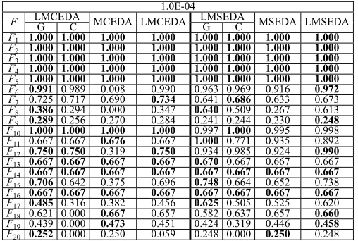
use-fulness of the dynamic cluster sizing strategy, we conduct comparison experiments between LMEDAs with the dynamic cluster sizing and the ones with different fixed cluster sizes. For these fixed sizes, to make it simple, we set them as {2, 4, 5, 6, 8, 10}, which is mainly for exact division. TableII
exhibits the comparison results between different versions of LMCEDA (the left part of the bolded line) and LMSEDA (the right part of the bolded line) with respect to PR at the accu-racy level ε=1.0E-04 and the best PR is highlighted in bold. The numbers under unit “LMCEDA” or “LMSEDA” denote
the fixed cluster sizes, and “dynamic” means LMCEDA or LMSEDA adopts the dynamic cluster sizing strategy.
Observing TableII, we can draw the following conclusions. 1) First, on F1–F5 and F13–F14, different cluster sizes make no difference on both LMCEDA and LMSEDA. However, on F6–F12, a small cluster size is preferred for both algorithms, and on F15–F20, neither a small nor a large cluster size is attractive, and only an appropriate cluster size is beneficial. This observation demonstrates that the optimal cluster size of different problems is not the same and such a size for different problems needs to be fine-tuned.
2) LMCEDA with the dynamic cluster sizing can achieve comparable performance on most problems (17 func-tions) when compared with the one with the optimal cluster size. The PR results obtained by the dynamic ver-sion on these functions are very close to those achieved by the one with the optimal cluster size. Specially, the dynamic version even obtains the best PR result on F17 and only loses the competition on F8 and F20.
3) LMSEDA with the dynamic cluster sizing shows its superiority to the one with the optimal cluster size. It achieves considerably similar PR results on 16 func-tions and obtains the best PR results on F6,F15,F17, and F19 in comparison with the version with the fixed optimal size.
In summary, the dynamic cluster sizing strategy is helpful for both LMCEDA and LMSEDA, and this benefit is more evident for LMSEDA. Such benefit comes from the potential balance between exploration and exploitation resulted from the changing cluster size. Additionally, the dynamic strategy on the cluster size also eliminates the sensitivity to this parameter and relieves users from the task of fine tuning.
2) Effects of Local Search and Combination of Distributions: Here, we take a close observation at the
influence of the local search scheme and the combi-nation of Gaussian and Cauchy distributions. In the experiments, we denote LMEDAs only with Gaussian distribution as LMEDA_Gs containing LMCEDA_G and LMSEDA_G. Likewise, LMEDAs only with Cauchy distribu-tion are denoted as LMEDA_Cs, including LMCEDA_C and LMSEDA_C. The proposed LMEDAs without local search are represented as MEDAs (MCEDA and MSEDA). The version with both techniques is still be LMEDAs (LMCEDA and LMSEDA). Table III presents the comparison results among these versions with respect to PR at accuracy level ε = 1.0E-04 with the left part of the bolded line related to LMCEDA and the right part associated with LMSEDA. The first two columns of each part, namely columns “G” and “C,” represent the results of LMCEDA_G (LMSEDA_G) and LMCEDA_C (LMSEDA_C), respectively. Additionally, the best PR results are highlighted in bold.
First, in terms of the combination of the two dis-tributions, comparing LMCEDA with LMCEDA_G and LMCEDA_C, we can see LMCEDA performs similarly to both LMCEDA_G and LMCEDA_C on 12 functions (F1–F6,
TABLE II
COMPARISONRESULTSABOUTPR BETWEENLMEDAS WITHDYNAMICCLUSTERSIZE ANDTHOSEWITH FIXEDCLUSTERSIZES ATACCURACYLEVELε=1.0E-04. THEBESTPR ISHIGHLIGHTED INBOLD
TABLE III
COMPARISONRESULTS INPR AMONGDIFFERENTVERSIONS OFMEDAS ATACCURACYLEVELε=1.0E-04 WITHBESTPR BOLDED
and F17–F20) functions, respectively. Besides, there is no loss of competition for LMCEDA in comparison with LMCEDA_C, and LMCEDA only seriously loses its advan-tage on F20when compared with LMCEDA_G. When it comes to LMSEDA, observing the right part, we find the combina-tion of the two distribucombina-tions is very beneficial, which helps LMSEDA defeat LMSEDA_G and LMSEDA_C on six func-tions (F6, F7, F9, F12, F18, and F19) and nine functions (F6, F8, F9, F11, F15, and F17–F20), respectively. And there is no serious loss of advantage for LMSEDA when compared with the two versions. Comprehensively, we can see the com-bination of the two distributions provides potential help for both LMCEDA and LMSEDA, and the benefit is more obvious on LMSEDA. Such benefit origins from the potential balance between exploration and exploitation afforded by the alterna-tive usage of the two distributions, which takes advantages of both distributions.
Second, from the perspective of the local search, compar-ing LMCEDA with MCEDA and LMSEDA with MSEDA,
respectively, which corresponds to the last two columns of the two parts, we can find that the local search is very useful for LMCEDA on F6, F8, F12, and F15, while it benefits LMSEDA specially on F6, F8, F12, F15, and F17. On other functions, even though such benefit is not evident, the perfor-mance of LMCEDA and LMSEDA is comparable to that of MCEDA and MSEDA, or even a little better, such as on F7,
F9, and F17 for LMCEDA and on F7, F9, F10, F18, and F19 for LMSEDA. As a whole, we can see that the local search scheme makes significant difference on both LMCEDA and LMSEDA.
In short, we can conclude that both the combination of the two distributions and the local search are beneficial for LMEDAs in locating more global optima.
3) Overall Performance of LMCEDA and LMSEDA: After
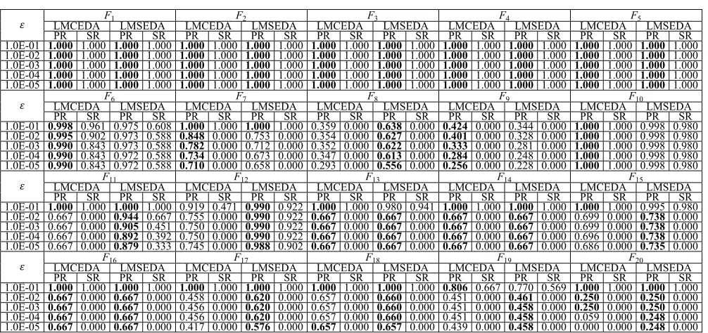
observing the influence of the three techniques on LMCEDA and LMSEDA from the above two series of experiments, we present the overall performance of these two algorithms at all accuracy levels. Table IV shows the comparison results between LMCEDA and LMSEDA with respect to PR and SR on all 20 functions at all accuracy levels and the best PR results are emphasized in bold.
From Table IV, we can observe the following.
1) Both algorithms achieve almost the same performance on nine functions (F1–F5, F10, F13, F14,and F16) at all five accuracy levels. Besides, on F1–F5, they can locate all known global optima successfully at any accuracy level, and on F10, LMCEDA can successfully find all global optima at all accuracy levels, while LMSEDA can nearly successfully locate all global optima with only one run missing finding only one global optima out of 51 independent runs. On F13, F14, and F16, both LMCEDA and LMSEDA can almost successfully find all global optima at accuracy level ε=1.0E-01, while at other levels, even though they cannot find all optima in any run, they are able to find most of the global optima (4 out of 6).
TABLE IV
COMPARISONRESULTS INPRANDSR BETWEENLMCEDAANDLMSEDAON20 FUNCTIONS ATDIFFERENTACCURACYLEVELS
LMSEDA on F7and F9. Conversely, LMSEDA displays its little superiority on F18 and F19, and wins the com-petition with great advantages on 6 functions (F8, F11,
F12, F15, F17, and F20).
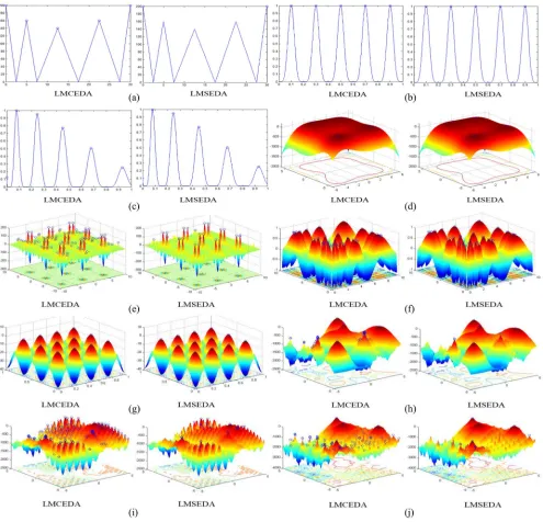
3) From the perspective of accuracy levels, both LMCEDA and LMSEDA can almost successfully locate all global optima for almost all functions at the accuracy level ε = 1.0E-01, except for F8, F9, F12, and F19 for LMCEDA and F6, F8, F9, and F19for LMSEDA. As for other accuracy levels, LMCEDA cannot achieve a suc-cessful run on 13 functions (F7–F9 and F11–F20) and LMSEDA cannot obtain any successful run on 11 func-tions (F7–F9 and F13–F20) owing to the influence of an ocean of local optima. Such phenomena is common for the state-of-the-art multimodal algorithms, but ours can locate more global optima in the unsuccessful runs, which will be testified in the following section. In addition, to have a better view of the comparison between LMCEDA and LMSEDA, we visualize the final fitness land-scape of the final population when the maximum number of fitness evaluations is exhausted on ten visual functions, which is shown in Fig.2.
First, we observe that both LMCEDA and LMSEDA can locate the global optima. And when there is not so many or even no local optima, as shown in Fig. 2(b)–(d), (f), and (g), LMCEDA and LMSEDA achieve very similar performance, namely the individuals are located around or at the global optima. However, when there are many or even masses of local optima, the two algorithms perform very differently. LMCEDA not only can locate global optima, but also can locate many local optima, while LMSEDA can locate more global optima but at the loss of locating local optima, which can be clearly seen in Fig. 2(e) and (h)–(j). Such phenom-ena may be attributed to the different individual selection
procedures adopted in LMCEDA and LMSEDA as shown in Algorithms 7 and 8, respectively.
In summary, we can conclude that from the perspective of locating more global optima as concerned in this paper, LMSEDA is a little superior to LMCEDA. But, from TableIV, we can see that both algorithms are promising for solving multimodal optimization problems.
C. Comparisons With State-of-the-Art Algorithms
To further demonstrate the superiority of LMEDAs (LMCEDA and LMSEDA), we conduct comparison experi-ments between LMEDAs and several state-of-the-art multi-modal algorithms. The compared algorithms are CDE [29], SDE [30], LIPS [41], R2PSO, R3PSO [42], Self_CCDE, Self_CSDE [37], NCDE, NSDE [38], LoICDE, LoISDE [40], and PNPCDE [39]. The brief description of these algorithms can be found in Section II-A. To make fair comparisons, the population size and the maximum number of fitness evalua-tions are set the same for all algorithms according to TableI. Other parameters introduced in the corresponding algorithms are set as recommended in the related papers.
For saving space, we leave all the comparison results at the five accuracy levels in the supplemental material. Tables SIII–SVII (in the supplemental material) show the comparison results with respect to PR, SR, and CS of dif-ferent multimodal algorithms at the five accuracy levels, and the best PRs are highlighted in bold. The row named “bprs” counts the number of functions where one algorithm obtains the best PR results, namely the number of bolded PRs. Tables SVIII–SXII (in the supplemental material) present nonparametric Wilcoxon rank-sum test2 results with respect to PR between LMEDAs and the state-of-the-art methods
Fig. 2. Comparison results in final fitness landscapes between LMCEDA and LMSEDA on ten functions that can be visualized. (a) F1. (b) F2. (c) F3. (d) F4. (e) F6. (f) F7. (g) F10. (h) F11. (i) F12. (j) F13.
at the five accuracy levels. In these tables, each compared algorithm is associated with two columns, of which the left are the results compared with LMCEDA and the right are the results compared with LMSEDA. In addition, the crit-ical value of Wilcoxon rank-sum test with respect to the rank sum for 51 samples is 2866. Therefore, the number larger than 2866 indicates that our algorithm is signifi-cantly better than the compared algorithm, and the number smaller than 2387 indicates our algorithm is significantly worse. Other cases mean our algorithm is equivalent to the compared algorithm. According to this standard, the grayed units in Tables SVIII–SXII (in the supplemental material) mean LMCEDA or LMSEDA is significantly better than the compared algorithm, while the bolded values indicate that LMCEDA or LMSEDA is significantly worse. Other cases
suggest LMCEDA or LMSEDA performs similarly to the com-pared method. On the basis of these, the last row (w/l/t) of these tables counts the number of functions on which LMCEDA or LMSEDA significantly wins, significantly loses, and ties the competitions when compared with corresponding counterparts.
Observing Tables SIII–SXII in the supplement material, we can draw the following conclusions.
PNPCDE, whose performance is comparable to both LMCEDA and LMSEDA at accuracy levelε=1.0E-01, decreases rapidly from 13, 15, 13, 15, and 13 to 8, 8, 10, 8, and 6, respectively, while that of LMSEDA keeps nearly unchanged. As the accuracy level changes from ε = 1.0E-02 to ε = 1.0E-05, LMSEDA always keeps its dominant position and performs significantly better than the other algorithms. When it comes to the last accuracy level, ε=1.0E-05, we can observe that both LMCEDA and LMSEDA outperform all the compared algorithms.
2) When we take a further look at Tables SIII–SVII (in the supplemental material), both LMCEDA and LMSEDA achieve the best performance on F15–F20, except for F20, on which LMSEDA obtains very sim-ilar result with NCDE, while LMCEDA receives poor performance. Such observation becomes more and more evident with the accuracy level increasing, which sub-stantiates the competitive efficiency and superiority of LMEDAs in dealing with larger and more complex search spaces, where masses of local optima exist. 3) When it reaches the comparison in CS, since it makes
no sense to evaluate this standard on functions where there is no successful run for one algorithm and on algorithms whose PR results are not comparable, we compare LMCEDA and LMSEDA only with CDE, NCDE, Self_CCDE, LoICDE, and PNPCDE on F1–F5, where they achieve comparable performance. At the first two accuracy levels, both LMCEDA and LMSEDA show no evident superiority to these five compared algorithms. However, when it arrives at the last three accuracy lev-els, we find that both LMCEDA and LMSEDA present their dominance to the five compared algorithms in CS. Take accuracy level ε = 1.0E-04 for example. From Table SVI (in the supplemental material), it can be found that LMCEDA achieves faster CS than CDE, NCDE, Self_CCDE, LoICDE, and PNPCDE on 3(F2,F3, and F5), 3(F1–F3), 3(F1–F3), 2(F2 and F3), and 3(F2,F3, and F5) functions, respectively, while LMSEDA converges faster than them on 3(F2,F3, and
F5), 3(F1–F3), 4(F1–F3and F5), 3(F2,F3, and F5), and 3(F2,F3, and F5) functions, respectively. This observa-tion potentially shows that LMEDAs can achieve a com-petitive convergence speed to locate global optima for multimodal optimization.
4) From Tables SVIII–SXII (in the supplemental mate-rial), we find that the dominance of both LMCEDA and LMSEDA to the counterparts becomes more and more obvious as the accuracy level increases. Specially, at the last accuracy level,ε=1.0E-05, both LMCEDA and LMSEDA are significantly better than all the com-pared algorithms on more than ten functions, except for NCDE and Self_CCDE. However, LMCEDA and LMSEDA still beat NCDE and Self_CCDE down on 7 and 8 functions, which is much more than the num-ber of functions where LMCEDA and LMSEDA are defeated by the two compared algorithms, respectively. Particularly, we find both LMCEDA and LMSEDA are
significantly superior to SDE, NSDE, and LoISDE on more than 17 functions. All these evidently ver-ify the superiority of LMEDAs to the state-of-the-art multimodal algorithms.
Comprehensively, we can conclude that with the accuracy level increasing, both LMCEDA and LMSEDA become more and more outstanding when compared with the state-of-the-art multimodal algorithms. This observation demonstrates that both LMCEDA and LMSEDA achieve consistent superiority at most accuracy levels, which can be attributed to the power-ful exploration ability and exploitation ability of LMEDAs, resulted from the three techniques proposed in this paper: 1) the dynamic cluster sizing; 2) the alternative usage of two distributions to generate offspring; and 3) the local search around seeds. Equipped with these strategies, LMEDAs can make a good balance between exploration and exploitation, which results in their efficiency and effectiveness in dealing with multimodal optimization problems.
V. CONCLUSION
This paper has developed MEDAs to locate multiple global optima for multimodal optimization problems. Distribution estimation and niching are effectively utilized to realize the proposed algorithms. Specially, the clustering-based niching tactics for crowding and speciation are incorporated, lead-ing to crowdlead-ing-based and speciation-based MEDAs, named MCEDA and MSEDA, respectively. Further, they are enhanced with local search, forming LMCEDA and LMSEDA, respec-tively. Their superior performance on multimodal problems is brought about by three techniques developed in this paper: 1) the dynamic cluster sizing; 2) the alternative usage of two distributions to generate offspring; and 3) the local search around seeds.
The niching methods of MEDAs are improved from those in the literature through developing a dynamic cluster-sizing strategy to afford a potential balance between exploration and exploitation, whereby relieving MEDAs from the sensitivity to the cluster size. Differing from classical EDAs to estimate the probability distribution of the whole population, MEDAs focus on the estimation of distribution at the niche level, and all individuals in each niche participate in the estimation of distribution of that niche. Further, the alternative usage of Gaussian and Cauchy distributions to generate offspring takes the advantages of both distributions, and potentially offers a balance between exploration and exploitation. Finally, the solution accuracy is enhanced through a new local search scheme based on Gaussian distribution with probabilities self-adaptively determined according to fitness values of seeds. The influence of these three techniques has been fully tested in the experiments. The comparison results with respect to PR, SR, and CS between MEDAs and the state-of-the-art multi-modal algorithms demonstrate the superiority and efficiency of MEDAs developed in this paper.
optima may be located when the dimensionality of the problem increases or there exist an excessive number of local optima. This directs certain future work in the development of MEDAs.
REFERENCES
[1] K.-C. Wong, K.-S. Leung, and M.-H. Wong, “Protein structure predic-tion on a lattice model via multimodal optimizapredic-tion techniques,” in Proc. Conf. Genet. Evol. Comput., Portland, OR, USA, 2010, pp. 155–162. [2] Q. Ling, G. Wu, and Q. Wang, “Restricted evolution based multimodal
function optimization in holographic grating design,” in Proc. IEEE Congr. Evol. Comput., Edinburgh, U.K., 2005, pp. 789–794.
[3] W. Sheng, S. Swift, L. Zhang, and X. Liu, “A weighted sum validity function for clustering with a hybrid niching genetic algorithm,” IEEE Trans. Syst., Man, Cybern. B, Cybern., vol. 35, no. 6, pp. 1156–1167, Dec. 2005.
[4] Y. Li, “Using niche genetic algorithm to find fuzzy rules,” in Proc. Int. Symp. Web Inf. Syst. Appl., Nanchang, China, 2009, pp. 64–67. [5] M. Boughanem and L. Tamine, “A study on using genetic niching for
query optimisation in document retrieval,” in Advances in Information Retrieval. Heidelberg, Germany: Springer, 2002, pp. 135–149. [6] E. Dilettoso and N. Salerno, “A self-adaptive niching genetic algorithm
for multimodal optimization of electromagnetic devices,” IEEE Trans. Magn., vol. 42, no. 4, pp. 1203–1206, Apr. 2006.
[7] D.-K. Woo, J.-H. Choi, M. Ali, and H.-K. Jung, “A novel multimodal optimization algorithm applied to electromagnetic optimization,” IEEE Trans. Magn., vol. 47, no. 6, pp. 1667–1673, Jun. 2011.
[8] J. Kennedy, “Bare bones particle swarms,” in Proc. IEEE SIS, Indianapolis, IN, USA, 2003, pp. 80–87.
[9] S. Das and P. N. Suganthan, “Differential evolution: A survey of the state-of-the-art,” IEEE Trans. Evol. Comput., vol. 15, no. 1, pp. 4–31, Feb. 2011.
[10] A. Zhou, J. Sun, and Q. Zhang, “An estimation of distribution algorithm with cheap and expensive local search methods,” IEEE Trans. Evol. Comput., vol. 19, no. 6, pp. 807–822, Dec. 2015.
[11] M. Hauschild and M. Pelikan, “An introduction and survey of estima-tion of distribuestima-tion algorithms,” Swarm Evol. Comput., vol. 1, no. 3, pp. 111–128, 2011.
[12] J. Kennedy, “Particle swarm optimization,” in Encyclopedia of Machine Learning. New York, NY, USA: Springer, 2010, pp. 760–766. [13] Z. Ren, A. Zhang, C. Wen, and Z. Feng, “A scatter learning particle
swarm optimization algorithm for multimodal problems,” IEEE Trans. Cybern., vol. 44, no. 7, pp. 1127–1140, Jul. 2014.
[14] K. Price, R. M. Storn, and J. A. Lampinen, Differential Evolution: A Practical Approach to Global Optimization. Heidelberg, Germany: Springer, 2006.
[15] Y. L. Li et al., “Differential evolution with an evolution path: A DEEP evolutionary algorithm,” IEEE Trans. Cybern., vol. 45, no. 9, pp. 1798–1810, Sep. 2015.
[16] N. Chen et al., “An evolutionary algorithm with double-level archives for multiobjective optimization,” IEEE Trans. Cybern., vol. 45, no. 9, pp. 1851–1863, Sep. 2015.
[17] W.-J. Yu et al., “Differential evolution with two-level parameter adap-tation,” IEEE Trans. Cybern., vol. 44, no. 7, pp. 1080–1099, Jul. 2014. [18] S.-Y. Park and J.-J. Lee, “Stochastic opposition-based learning using a beta distribution in differential evolution,” IEEE Trans. Cybern., in press.
[19] W. Du, S. Y. S. Leung, Y. Tang, and A. V. Vasilakos, “Differential evolution with event-triggered impulsive control,” IEEE Trans. Cybern., in press.
[20] M. Srinivas and L. M. Patnaik, “Genetic algorithms: A survey,” Computer, vol. 27, no. 6, pp. 17–26, Jun. 1994.
[21] X.-Y. Zhang et al., “Kuhn–Munkres parallel genetic algorithm for the set cover problem and its application to large-scale wireless sensor networks,” IEEE Trans. Evol. Comput., in press.
[22] W.-N. Chen et al., “Particle swarm optimization with an aging leader and challengers,” IEEE Trans. Evol. Comput., vol. 17, no. 2, pp. 241–258, Apr. 2013.
[23] J. Kennedy and R. Eberhart, “Particle swarm optimization,” in Proc. IEEE Int. Conf. Neural Netw., vol. 4. Perth, WA, Australia, 1995, pp. 1942–1948.
[24] Y.-J. Gong et al., “Genetic learning particle swarm optimization,” IEEE Trans. Cybern., in press.
[25] W.-N. Chen et al., “A novel set-based particle swarm optimization method for discrete optimization problems,” IEEE Trans. Evol. Comput., vol. 14, no. 2, pp. 278–300, Apr. 2010.
[26] A. Pétrowski, “A clearing procedure as a niching method for genetic algorithms,” in Proc. IEEE Congr. Evol. Comput., Nagoya, Japan, 1996, pp. 798–803.
[27] G. R. Harik, “Finding multimodal solutions using restricted tournament selection,” in Proc. Int. Conf. Genet. Algorithms, Pittsburgh, PA, USA, 1995, pp. 24–31.
[28] D. E. Goldberg and J. Richardson, “Genetic algorithms with shar-ing for multimodal function optimization,” in Proc. Int. Conf. Genet. Algorithms, Cambridge, MA, USA, 1987, pp. 41–49.
[29] R. Thomsen, “Multimodal optimization using crowding-based differen-tial evolution,” in Proc. IEEE Congr. Evol. Comput., vol. 2. Portland, OR, USA, 2004, pp. 1382–1389.
[30] X. Li, “Efficient differential evolution using speciation for multi-modal function optimization,” in Proc. Conf. Genet. Evol. Comput., Washington, DC, USA, 2005, pp. 873–880.
[31] J.-P. Li, M. E. Balazs, G. T. Parks, and P. J. Clarkson, “A species con-serving genetic algorithm for multimodal function optimization,” Evol. Comput., vol. 10, no. 3, pp. 207–234, 2002.
[32] C. Stoean, M. Preuss, R. Stoean, and D. Dumitrescu, “Multimodal opti-mization by means of a topological species conservation algorithm,” IEEE Trans. Evol. Comput., vol. 14, no. 6, pp. 842–864, Dec. 2010. [33] C. L. Stoean, M. Preuss, R. Stoean, and D. Dumitrescu, “Disburdening
the species conservation evolutionary algorithm of arguing with radii,” in Proc. Conf. Genet. Evol. Comput., London, U.K., 2007, pp. 1420–1427.
[34] J. Gan and K. Warwick, “Dynamic niche clustering: A fuzzy variable radius niching technique for multimodal optimisation in GAs,” in Proc. IEEE Congr. Evol. Comput., Seoul, Korea, 2001, pp. 215–222. [35] Y. Jie, N. Kharma, and P. Grogono, “Bi-objective multipopulation
genetic algorithm for multimodal function optimization,” IEEE Trans. Evol. Comput., vol. 14, no. 1, pp. 80–102, Feb. 2010.
[36] L. Li and K. Tang, “History-based topological speciation for multimodal optimization,” IEEE Trans. Evol. Comput., vol. 19, no. 1, pp. 136–150, Feb. 2015.
[37] W. Gao, G. G. Yen, and S. Liu, “A cluster-based differential evolution with self-adaptive strategy for multimodal optimization,” IEEE Trans. Cybern., vol. 44, no. 8, pp. 1314–1327, Aug. 2014.
[38] B. Y. Qu, P. N. Suganthan, and J. J. Liang, “Differential evolution with neighborhood mutation for multimodal optimization,” IEEE Trans. Evol. Comput., vol. 16, no. 5, pp. 601–614, Oct. 2012.
[39] S. Biswas, S. Kundu, and S. Das, “An improved parent-centric mutation with normalized neighborhoods for inducing niching behavior in differ-ential evolution,” IEEE Trans. Cybern., vol. 44, no. 10, pp. 1726–1737, Oct. 2014.
[40] S. Biswas, S. Kundu, and S. Das, “Inducing niching behavior in differ-ential evolution through local information sharing,” IEEE Trans. Evol. Comput., vol. 19, no. 2, pp. 246–263, Apr. 2015.
[41] B. Y. Qu, P. N. Suganthan, and S. Das, “A distance-based locally informed particle swarm model for multimodal optimization,” IEEE Trans. Evol. Comput., vol. 17, no. 3, pp. 387–402, Jun. 2013. [42] X. Li, “Niching without niching parameters: Particle swarm
optimiza-tion using a ring topology,” IEEE Trans. Evol. Comput., vol. 14, no. 1, pp. 150–169, Feb. 2010.
[43] X. Liang, H. Chen, and J. A. Lozano, “A Boltzmann-based estimation of distribution algorithm for a general resource scheduling model,” IEEE Trans. Evol. Comput., vol. 19, no. 6, pp. 793–806, Dec. 2015. [44] S. Shahraki and M. R. A. Tutunchy, Continuous Gaussian Estimation
of Distribution Algorithm (Advances in Intelligent Systems and Computing). Heidelberg, Germany: Springer, 2013, pp. 211–218. [45] P. Yang, K. Tang, and X. Lu, “Improving estimation of distribution
algorithm on multimodal problems by detecting promising areas,” IEEE Trans. Cybern., vol. 45, no. 8, pp. 1438–1449, Aug. 2015.
[46] D. Weishan and Y. Xin, “NichingEDA: Utilizing the diversity inside a population of EDAs for continuous optimization,” in Proc. IEEE Congr. Evol. Comput., Hong Kong, 2008, pp. 1260–1267.
[47] Y. Wang, H.-X. Li, G. G. Yen, and W. Song, “MOMMOP: Multiobjective optimization for locating multiple optimal solutions of multimodal opti-mization problems,” IEEE Trans. Cybern., vol. 45, no. 4, pp. 830–843, Apr. 2015.