PARAMETERISATION COMPARISON FOR THE DETECTION OF PANIC DISORDER USING TIME-FREQUENCY TRANSFORMS AND SUPPORT VECTOR MACHINES
H. Dietl1and S. Weiss1
1Communications Research Group, ECS, University of Southampton, Southampton, United Kingdom
[email protected], [email protected]
Abstract: In this paper we compare the effect of the parameterisation on the automatic detection of diseases based on biomedical data. Exemplarily, we study the analysis of event related brain potentials in patients suf-fering from panic disorder, whereby the data comprises responses to neutral and panic causing stimuli. This data is parameterised by time-frequency (TF) transforms, from which features are selected by a statistical test. The selected features represent the input to a support vector machine classifier yielding a detection rate for the TF parametrised data. This is compared with detection rates obtained for unparameterised time domain data.
Keywords: Transient, evoked, otoacoustic, emissions, wavelet, support, vector, machines.
INTRODUCTION
In medical facilities it is a common issue to judge the re-sponses of patients to stimuli in order to determine a po-tential physiological or psychological illness [1, 2]. In cases where the response can be measured as an elec-trical signal, the signal evaluation used to be primarily based on an expert’s decision regarding the waveforms of averaged signals. Such waveforms and often parameters derived from these as presented by standard clinical mea-surement devices were treated as additional information only. Recently, however, automated evaluation methods based on signal processing approaches have more and more frequently enhanced or even replaced the expert’s judgement [1, 3]. As a result, many different propositions were made concerning statistical signal evaluation in an effort to enhance or perhaps even replace the decision of a human expert.
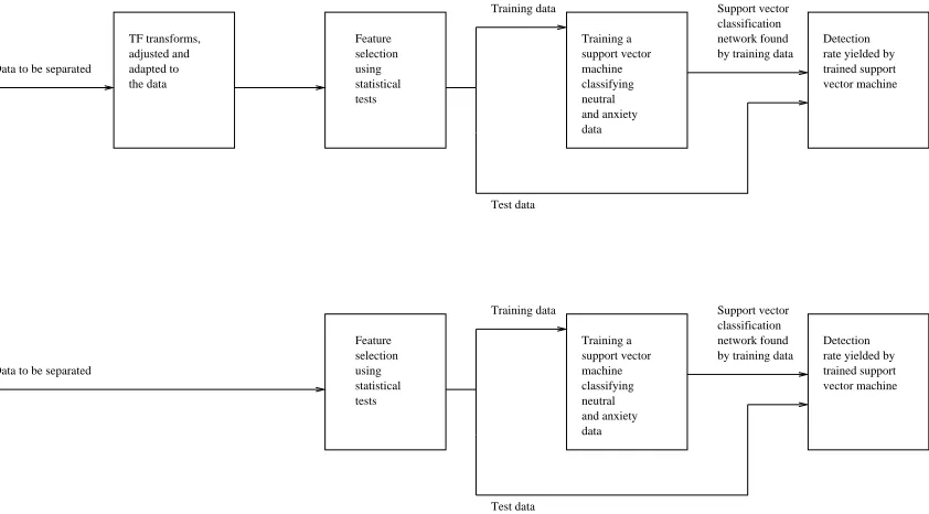
Here, we contribute to evaluate the separation of biomedical data to detect potential illnesses by firstly showing the application of TF methods and statistical tests to select features as introduced in [3]. Then, the selected features are used as an input to a support vector machine classifier which returns a trained support vector classification network. Using this network, a detection rate for a test data group is received. This method, as out-lined in Fig. 1 is applied to panic disorder data collected from one patient. We are especially interested in investi-gating the influence of the parameterisation and therefore, we compare the detection results received for the selected features based on the TF parameterisations and unparam-eterised time domain data. As the amount of panic dis-order data is limited, the TF transforms as well as the statistical tests are applied to all available data, before it
is split into training and test data sets, as illustrated in Fig. 1 to ensure a robust parameterisation. However, as the main purpose of this contribution is to evaluate the pa-rameterisation, the drawback compared to a study where the parameterisation is based on a training data set only can be accepted.
The paper is organised as follows. Firstly, we will introduce the TF transforms for the parameterisation of the data. Then, a method to isolate indicative parameters, which can be used for distinguishing is discussed. Next, we describe the support vector machine classifier which gives a detection rate for the test data based on a network resulting from the training data. The test and training data are received by splitting the data used for identifying dis-tinctive coefficients. The paper closes with test results and conclusions for the application to panic disorder and acknowledgements.
TRANSFORMATION METHODS
In the following, we discuss transform methods to para-metrise biomedical data with the aim of expressing its features by as few coefficients as possible.
To take the transient nature of biomedical waveforms into account, TF transforms are used for parameterisa-tion of the data. For our applicaparameterisa-tion to panic disorder, TF transforms with a good time resolution are required [3]. The discrete wavelet transform (DWT) however gener-ally yields a good frequency resolution and poor time res-olution at low frequencies, resulting in a too coarse time segmentation in the frequency range of interest. There-fore, we concentrate on wavelet packet (WP) transform, whose level of decomposition can be adapted to fit the na-ture of the data, as well as the Gabor Frame (GF) decom-position, which yields a uniform tiling of the TF plane and hence can provide a desired resolution in a specific TF segment.
For the transforms considered, we choose a matrix no-tation
y=Tj·x , (1)
wherexrepresents one discrete and finite measurement in the time domain withN elements,yis vector holding the transformation coefficients andj = {WP,GF}the potential transform method. While fast implementations of WP [4] and GF [5] avoid matrix implementations, the calculation of a limited number of significant elements inycan be performed faster by extracting the according rows fromTj. As the data inx is finite, a symmetric
Feature selection using
tests statistical
Data to be separated trained support
support vector machine
and anxiety classifying neutral
data
by training data network found
Test data
Detection rate yielded by
vector machine Feature
selection using
tests statistical TF transforms,
adjusted and adapted to the data
Data to be separated trained support
support vector machine
and anxiety classifying neutral
data
by training data network found
Test data
Detection rate yielded by
vector machine Training data
Training data
classification Support vector
Support vector classification Training a
[image:2.595.91.512.67.300.2]Training a
Fig. 1: Overview: Detection comparison study for (top) parameterised data and (bottom) time domain data.
Discrete Wavelet and Wavelet Packet Transformation The WP is based on a discrete wavelet transformation (DWT) which is a fixed transform based on a “mother wavelet” from which the transformation coefficients are derived by scaling, translation and sampling. To comply with the symmetric extension inTj, the mother wavelet
must be symmetric. Here, we have chosen the Mallat wavelet [4] for which good results have been reported in similar studies [1]. We firstly review the DWT very briefly to lay the foundation for the description of the WP. The DWT transform with a matrixTDWT ∈RK×N
results in the vectory[k]∈RK
y=
y[0] y[1] · · · y[K−1]T
(2)
containing the DWT coefficientsy[k],k = 0(1)K−1 of the vectorxwithK =N. Each coefficient approxi-mately covers a TF tile in Fig. 2a).
The WP transform is an adaptive transformation simi-lar to the DWT but with a different partitioning of the TF plane. The advantage of this approach compared to the DWT is that the entropy ofyshall be minimised through variable levels of decomposition such that the energy is concentrated in as few coefficients as possible. One suit-able measure for such a concentration is given by the Shannon entropy
(y) =− K−1
X
k=0
ln(kyk2)· kyk2, (3)
where ln is the natural logarithm andkykthe Euclidean vector norm ofy. The adaptive transformation approach is implemented in the following way: The measure in (3) is calculated for every wavelet decomposition level and if the entropy is decreased from one decomposition to the next, the decomposition will be continued. If the
[image:2.595.313.536.417.557.2]entropy from one decomposition level to the next does not decrease, the decomposition will be stopped.
Fig. 2 shows a sample DWT and WP decomposition, whereby the DWT can be considered as a special case
Time 1 1 1 1 1 1 1 1
2 2 2 2
3 3
4 4
1 1 1 1 1 1 1 1
2 2 2 2
3 3
3 3
Frequency
Level 1
Level 3
Level 4 Level 2
Frequency
Level 1
Level 3
Time
Level 2 Level 3
Level 4
Fig. 2: Time-frequency tiling comparison between a) a DWT and b) a sample WP decomposition
of the WP transformation where the TF plane is seg-mented dyadically form one level to the next. The matrix TWP ∈ RK×N is found as follows: For each
measure-ment vectorxto be transformed, the WP decomposition is calculated. Then, the decomposition that shows the minimum entropy averaged over all measurements is se-lected among the decompositions for each measurement as the optimal WP decomposition. The difference be-tween the wavelet matrixTDWTand the wavelet packet
matrixTWP lies in the change of some rows. For the
example in Fig. 2, the rows that contain the level 2 coef-ficients inTDWT are replaced by level 3 coefficients in
Gabor Frames
The GF are the second transform method applied to the data. This transform is fixed and its main difference compared to the WP is that the GF parametrisation is overcomplete and yields complex valued transform co-efficients. We can also choose from various prototype functions to find the best one matching our analysis. The transform implemented here is an oversampled gener-alised DFT filter bank according to [5]. The GF trans-form can be regarded as a short time Fourier transtrans-form with more restrictions for the translated window, which is the prototype filter for the GF. Fig. 3 shows a sample time frequency tiling, which is characterised by the uni-form resolution of the GF. Gabor functions are derived
Frequency
Time
Fig. 3: Time frequency tiling for GF
from a prototype functionh[n]by modulation, usually
hm[n] =h[n]·ejΩmn, (4)
and give a decomposition according to
ym[k] =
X
n
x[k·D−n]·hm[n], (5)
whereDis the decimation factor.
As an example for a GF via an oversampled gener-alised DFT filter bank [5] let us assume a filter length of W = 448 for the prototype function, a frequency segmentation ofS = 32 uniform scales, a decimation
D = 28and length of the vectorxofN = 224. This setting yields a transform matrix TGF ∈ CK×N with
K = (N/D + 1)·S/2,K = (22428 + 1)· 322 = 144. Similar to a DFT, this type of transform yields a symme-try in the transform parameters for real valued input data. Hence, in general only half of the coefficients need to be retained, as the remainder is complex conjugated only and therefore redundant which is represented by the term
S/2in the formula above. Filters with varying length, frequency and time segmentations are used to determine a matrixTGF that optimises the parametrisation of the
data. Apart from the restrictions thatN needs to be an integer multiple ofDandW/Kneeds to be an even inte-ger, there are no other constraints in terms of the length of the signal to be analysed and the length of the analysing filter. This can be regarded as advantageous.
DIFFERENCE EVALUATION
Based on the various parameterisations derived in the pre-vious section, we will identify a set of coefficients that allows us to differentiate between the presented neutral and anxiety words.
F-Test
Prior to the selection of significant coefficients that repre-sent the main characteristics of the data, anF-test [7] is conducted to determine which method is used to identify them. The aim of this test is to determine whether two data sets are sampled from normal distributions with the same variances. If a value for the significance levelP of lower than0.05is obtained by theF-test, we conclude that the hypothesis is rejected and the two data sets are sampled from normal distributions having different vari-ances. The value ofP = 0.05is a limit commonly used in medical research [7]. When the setsx1 andx2
con-tain the series for one transformed coefficientk for all measurements taken for data set 1 representing the num-ber of presented neutral words and data set 2 representing the number of presented anxiety words, they can be com-pared by theF-value, which is given by [7]
F = σ
2 1
σ2
2
, (6)
withσ2
1 andσ22being the variances of the two data sets.
To receive the significance levelPfor theF-test, we need to define the degrees of freedom for the two data sets ac-cording to
ν1 = L1−1 and
ν2 = L2−1, (7)
withL1andL2being the number of samples,ν1the
de-grees of freedom for the data set 1 andν2the degrees of
freedom for the data set 2. With theF value defined by (6) and the degrees of freedomν1andν2, the significance
levelPfor theF-test can be determined from lookup ta-bles in literature, e.g. [7]. The tabulated values ofF are all greater than1, the two data sets in (6) need to be la-belled such thatσ2
1 ≥σ22. If the outcome of theF-test
confirms that the two data sets are sampled from distribu-tions with equal variances, we can subsequently conduct at-test to determine distinctive coefficients. If the re-sult of theF-test is that the underlying distributions from which the two data groups are sampled possess different variances we conduct aut-test. Thet-test and theut-test are defined in the next subsection.
t- andut-Tests
sig-nificance is returned. Thet-value is defined as [7]
t= qx1−x2
σ2 1
L1+
σ2 2
L2
= x1−x2
σq1
L1+ 1
L2
, (8)
withσ2=σ2
1 =σ22. The valuesx1andx2represent the
means for the two data sets, according to
xi=
1
Li
· Li−1
X
l=0
xi[n], i∈ {1,2}, (9)
withxTi = [xi[0]xi[1]... xi[Li−1]].
Thet-value also corresponds to a certain significance levelP, which can be looked up from tables [7], with the degrees of freedom defined by νt = ν1 +ν2 =
L1+L2−2. A smaller value forP indicates that the
data sets have a significantly different mean. For exam-ple, forP = 0.01the probability that the differences in the means are due to a sampling error is 1%. To iden-tify distinctive coefficients for our study, the determina-tion of the applied significance level will be discussed in the next subsection. The two tested distributions for our study were the distributions for a specific transform pa-rameter over the two data sets.
For the case that theF-test yields a difference in vari-ances such that thet-test cannot be used, we apply aut -test for unequal variances defined as
ut=qx1−x2
σ2 1
L1 + σ2
2
L2
. (10)
According to [7], for data sets sampled from distributions with unequal variances, thetdistribution can be approx-imated by theutvalue if thettable is entered at the fol-lowing defined degree of freedom:
νut=
(σ2
1/L1+σ22/L2)2 (σ2
1/L1)2
L1−1 + (σ2
2/L2)2
L2−1
. (11)
This test tends to be less powerful than the usualt-test, since it uses fewer assumptions [7]. However, for our ap-plication to panic disorder data, all identified distinctive coefficients have been isolated by the t-test. The main purpose of theut-test is to have an analysis tool for all coefficients at hand whether they show equal variances or not.
To determine a significance level P, the relation of the t-test to the receiver operating characteristic (ROC) analysis is shown in the next subsection.
Relation Between ROC Analysis andt-Test
We firstly describe the receiver operating characteristic (ROC) analysis and then introduce the connection be-tween ROC curves and thet-test and how we used the ROC analysis for our system.
A good measure for differentiation between two dis-tributions are ROC curves [8], since the area under the ROC curve measures the separability independent of the
selection of any threshold. Therefore, they have become remarkably useful in medical decision-making [8].
Firstly, we start by introducing the terms sensitivity and specificity [8] as we refer to these terms later when showing the results of our study. We assume we a have population consisting of healthy controls and patients that suffer from a certain disease but do not know or cannot express their suffering (e.g. hearing loss in infants). Our goal is to determine the patient group out of the tion. For this, we run an imaginary test on the popula-tion. The outcome of the test consists of one test parame-ter which is either positive indicating the tested person is sick or negative meaning the tested person is healthy. In order to evaluate the performance of that test, the follow-ing values can be used, as illustrated in Table 1.
The interrelationship equations in the table result from the fact that each person is classified as healthy or sick by the test. In the following the terms represented in the table will be used equivalently, meaning that we always refer to the true positive rate when speaking of sensitivity or hit rate.
Secondly, we continue by introducing the ROC curves. An ROC curve is a graphical representation of the trade off between sensitivity and specificity for every possible cut off. By tradition, the plot of the ROC curve shows the false positive rate on the x axis and the hit rate on the y axis. However, based on the interrelationships shown in Table 1, the axis of the ROC curve can be mod-ified. Suppose the above mentioned test parameter yields distributions for the sick and healthy groups as illustrated in Fig. 4 on the left.
The solid line represents the distribution of the test pa-rameter for the patient group, the dashed line for healthy
−6 −4 −2 0 2 4 6 0
0.2 0.4 0.6 0.8 1
size of test parameter
quantity
0 20 40 60 80 100 0
20 40 60 80 100
false alarm rate / [%]
sensitivity / [%]
d=2
0.9220 F=
−6 −4 −2 0 2 4 6 0
0.2 0.4 0.6 0.8 1
size of test parameter
quantity
0 20 40 60 80 100 0
20 40 60 80 100
false alarm rate / [%]
sensitivity / [%]
d=0.1
0.5289 F=
Fig. 4: ROC explanation: sample distributions (left) for sick (solid) and healthy (dashed) groups assuming an imaginary test parameter yielding ROC curves (right).
Test for disease interrelationship
sick group healthy group
Test result: true positive (TP) rate in %, false positive (FP) rate in %, TP + FN = 100% positive sensitivity, hit rate false alarm rate
Test result: false negative (FN) rate in % true negative (TN) rate in %, TN + FP = 100%
negative specificity
Table 1: Definition of sensitivity and specificity.
the false alarm rate as axis labels. The false alarm rate describes the specificity as shown in Table 1. The lower case shows the same but ford= 0.1.
Ideally, for a good separation, the sensitivity and the specificity should be very high. As Fig. 4 illustrates, a value for the area under the ROC curve close to 1 yields a relatively good separation, whereas a value close to 0.5 yields a very poor performance when taking both the sen-sitivity and separability into account.
Having introduced the ROC analysis, we continue by showing a connection between the area under the ROC curve and the significance level received by thet-test.
Here, we make use of the ROC analysis to evaluate and obtained a significance level for the t-tests or ut -tests. Moreover, for finding a prototype filter for the GF transform, the ROC analysis is applied. The relation is investigated as follows. Different values for the area un-der the ROC curve are determined. For these values, two Gaussian distributions are generated. From these distri-butions, a certain number of random samples are taken out and based on at-test orut-test, the significance level is calculated for these samples originating from the Gaus-sian distributions. This calculation is repeated with ran-dom samples from the distributions and the significance level is averaged until it converges. The ROC analysis is independent of the sample size whereas thet-test and
ut-test depend on it. Therefore, different sample sizes yield different relations, which is illustrated in Fig. 5 for a significance levelP received by thet-test. When using theut-test to investigate this relation, the results are very similar, e.g. no differences can be observed when adding the resulting curves to the ones illustrated in Fig. 5.
For our analysis of the panic disorder, we deal with a sample size of 24. Table 2 shows the areas under the ROC curve for the most commonly used significance lev-elsP [7] in more detail.
Area under the ROC curve Significance levelP
0.717 0.05
0.778 0.01
Table 2: Area under ROC curve and significance levels
Pfor a sample size of 24.
In most social research significance levels of P = 0.05orP = 0.01are used to determine difference be-tween two sets of data [7]. In other studies such as [1], ROC values of≈ 0.77are found and stated to yield ac-ceptable separation performance. Therefore, we choose
0.680 0.7 0.72 0.74 0.76 0.78 0.8 0.82 2
4 6 8 10 12
ROC area value
Significance Level P / %
sample size of 18 sample size of 21 sample size of 24 sample size of 27 sample size of 30 sample size of 33
Fig. 5: Significance LevelPfort-test over area under the ROC curve value for different sample sizes.
a significance level ofP = 0.01 for our study to ob-tain distinctive transform coefficients. Also, when test-ing different prototype filters for the GF transform, we choose the one having the largest ROC value for the iso-lated transform coefficients. Next, we discuss the support vector machine classifier we applied.
SUPPORT VECTOR MACHINES
In the following, we give a brief introduction to support vector machines. For a detailed description, we refer to [9, 10]. We consider a two class classification problem, namely one class defined by anxiety causing data, and one class describing neutral data, which is split into two data groups, namely training data and test data, respec-tively. The training data is described as a set of training vectors {pi}i=1... M with corresponding binary labels Si = 1for the one class, e.g. neutral data, andSi =−1
for the second class, e.g. anxiety causing data. The SVM conducts a classification of a test vectortby assigning a labelSˆby calculating
ˆ
S=sign(f(t)) with f(t) =X
i
αiSiK(t,pi)+b.
(12) The αi are called weights and b is the bias, which are
SVM parameters and adopted during training by max-imising
LD=
X
i
αi−
1 2
X
i,j
under the constraints
0≤αi≤C and
X
i
αiSi= 0 (14)
withC being a positive constant which weighs the in-fluence of training errors. K(·,·)is called kernel of the SVM. If there is a solution for αi, a value for bis
de-termined. There are several commonly used kernels for SVM, which give some flexibility for the underlying ap-plication. Many implementations of kernels can be found in literature, whereby two popular ones are:
• Gaussian kernel:
K(pi,pj) =exp(−γkpi−pjk2),
• polynomial kernel:K(pi,pj) = (pTi ·pj)d,
whereγis a kernel parameter for the Gaussian kernel and
dthe order of the polynomial kernel.
IfK(·,·)is positive definite, (13) and (14) is a con-vex quadratic optimisation problem, which converges to-wards the global optimum assuringly. This optimisation can be quite demanding in terms of computation time for real-world problems, and therefore, sophisticated algo-rithms like the sequential minimal optimisation (SMO) [9] are used for the solution.
Usually αi = 0 for the majority ofi and thus the
summation in (12) is limited to a subnet of thepi, which
therefore is called the set of support vectors. For Gaus-sian kernels, when using stretched out values for the lim-itation of training errors defined byCand the kernel pa-rameterγ, so called overfitting can occur meaning that all
M training vectors are identified as support vectors. To avoid this for our application, we have chosen to use the polynomial kernel of orderd= 3as this is assumed to be the best comprise between computational time, avoiding overfitting and yielding a good detection rate for the test data.
RESULTS AND DISCUSSION
As discussed previously, we have different transform methods and a procedure to identify significant coeffi-cients to being able to separate biomedical data. When splitting the data arbitrary in training and test data and ap-plying a support vector machine as described in the previ-ous section, we yield specific detection rates for training data as well as for the test data where the results for the test data describe the generalisation of the support vector classification network. We can also apply the tests de-scribed to unparameterised time domain data, deploy the support vector machine classification method and yield detection results for unparameterised data. By doing so, we arrive at an evaluation of the parameterisation meth-ods. In the following, we will show this procedure ap-plied to panic disorder data.
Description of the Data
Individuals with panic disorder are characterised by an abnormal fear of certain anxiety connected sensations
such as palpitation, breathlessness, or dizziness [2]. The research into this disorder has led to studies investigating its symptoms by means of appropriate stimulation and measurement of the subsequent event related brain po-tentials [3]. In this context, visual stimulation has been performed with words causing panic disorder, whereby the EEG can be recorded showing event related poten-tials (ERP). Previous studies have resulted in revealing a low frequent transient waveform appearing approxi-mately 300 ms after stimulus onset as a distinctive char-acteristic which is referred to as P300.
For our study, panic disorder ERP were measured for an anxiety patient who was presented with fear-inducing or neutral words tachistoscopically at the per-ception threshold of panic disorder. The patient’s percep-tion threshold for correctly identifying 50% of the words was determined with neutral words not used in the exper-iment. It can be assumed that the patient will recognise a greater number of anxiety words given at his perception threshold than neutral words [2]. Thus, it can be expected that the EEG exhibit an difference when neutral and anx-iety words are presented.
The EEG was measured at the vertex electrode (Cz) synchronously to the stimuli, whereby the recordings were started 100 ms before the onset of the visual word stimulus. The data exemplary analysed in this study contains 24 neutral word presentations and 24 anxiety word presentations to one panic patient. Fig. 6 shows the average over the stimulus-synchronous EEG in reac-tion to the 24 words presented for each word category. The figure reveals a difference in the two averages with a stronger P300 and more positive EEG until approxi-matelyt= 700ms in the panic disorder related data.
0 0.2 0.4 0.6 0.8 1 1.2 1.4 1.6 1.8 2
−5 0 5 10 15
time / [s]
voltage / [
µ
V]
Average over presented neutral words Average over presented anxiety words
Fig. 6: Average over 24 EEG segments showing re-sponses to anxiety related and neutral stimuli at the per-ception threshold.
Transform Adjustment
Identified Coefficients and Difference Comparison The coefficients to which the difference evaluation is ap-plied were preselected whereby only coefficients are con-sidered which contain85%of the total energy. This is reasonable, as it reduces the probability to identify coef-ficients that contain noise only.
Fig. 7 shows the resulting coefficients when perform-ing the difference evaluation on the parameterised data. The coefficients cover approximately the area of the P300 slow wave as it can be expected. They are all identified via at-test according to a priorF-test whereby the thresh-old for the significance level for theF-test wasP = 0.05, and for thet-test, it was set toP= 0.01.
For the unparameterised time domain data, 18 coeffi-cients were identified, where the same statements as for the parameterised data apply.
Fig. 8 shows the difference of the averages of the neu-tral and anxiety EEG compared with its parameterisa-tion by the identified coefficients for the two investigated transforms and for unparameterised time domain data.
It can be observed that the identified coefficients pa-rameterise the P300 better for the WP than for the GF. However, the GF seems to show a better parameterisation than time domain data. In order to evaluate these results, a SVM analysis is applied next.
Detection Rates Yielded by SVM
As explained in the SVM section, a polynomial kernel of order 3 was used for the SVM. To find a significant value for the training errorC, a leave-one-out (l-o-o) estimation of the error rate is applied as follows: From the training samples, remove the first example. Train the SVM on the remaining samples. Then test the removed example. If the example is classified incorrectly, it is said to produce a leave-one-out error.
In [9], an approach to estimate the maximum l-o-o er-ror is shown avoiding training the SVM more than once, which is also used for our study. By changing the value forCstepwise, the minimum for the l-o-o error is found determining the SVM classification network.
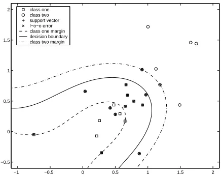
Fig. 9 shows a SVM classification with a minimised l-o-o error for a WP parameterisation. This can be shown in a two dimensional plane as the for the WP, two coeffi-cients were identified as significant. The two coefficoeffi-cients are illustrated in Fig. 7 (left).
In Fig 9, one class is defined by 12 points originating from arbitrary chosen neutral words and the second class
time / [s]
frequency / f
S
0 0.5 1 1.5 2 0
0.05 0.1
time / [s]
frequency / f
s
0 0.5 1 1.5 2 0
[image:7.595.315.541.68.249.2]0.05 0.1
Fig. 7: Resulting coefficients for (left) WP and (right) Gabor transforms.
0 0.2 0.4 0.6 0.8 1 1.2 1.4 1.6 1.8 2 −5
0 5
voltage / [
µ
V]
WP reconstruction difference
0 0.2 0.4 0.6 0.8 1 1.2 1.4 1.6 1.8 2 −5
0 5
voltage / [
µ
V]
GF reconstruction difference
0 0.2 0.4 0.6 0.8 1 1.2 1.4 1.6 1.8 2 −5
0 5
time / [s]
voltage / [
µ
V]
[image:7.595.316.535.556.732.2]time reconstruction difference
Fig. 8: Difference of neutral and anxiety EEG data com-pared with its parameterisation identified by thet-test for (top) WP, (middle) Gabor transforms and (bottom) unpa-rameterised time domain data.
represents 12 panic causing words, also chosen arbitrary from the whole 24 defining one training data set. For this example, class one is completely assigned correctly; class two gets assigned incorrectly in13of all cases. This rather asymmetric decision is due to the comparably small data size. Therefore, the SVM classification was conducted 100 times and averaged at the end meaning in loop, 12 arbitrary measurements for the two data groups were cho-sen, the SVM trained and the test group consisted of the remaining 12 measurements for each word category. Ta-ble 3 shows the results for this procedure for the training data.
It can be seen that the time domain data and the WP parameterisation yield comparably high values, whereas the GF identifies around two out of three words correctly for the training data. The number of support vectors is similar for each case.
−1 −0.5 0 0.5 1 1.5 2 −0.5
0 0.5 1 1.5
[image:7.595.61.286.678.739.2]2 class one class two support vector l−o−o error class one margin decision boundary class two margin
time GF WP domain transform transform sensitivity 99.55 % 66.78 % 92.00% specificity 93.13 % 65.88 % 96.28% number of 15.68 16.65 17.39 support vectors
Table 3: Results for training data.
Next, the more interesting results for the test groups are presented in Table 4. It can be seen that the WP
time GF WP
domain transform transform sensitivity 67.34 % 78.49 % 82.32% specificity 55.63% 54.39 % 52.82%
Table 4: Results for test data.
shows the overall best detection results for the test data, followed by the GF and the time domain data perform-ing worst. However, for the specificity all three cases are similar around50%.
What can be expected from Fig. 8 is confirmed: The WP parameterisation yields the best detection rates, fol-lowed by the GF transform and the simple time domain data performing worst. However, the specificity for the TF-transforms is not significant although the test data is used for the adjustment of the parameterisation meth-ods. This can be due to the relatively small amount of data available. Moreover, thet-test for receiving distinc-tive coefficients may not be powerful. Therefore, the de-scribed system might show more encouraging results for the analysis of biomedical data which comprises more measurements than here and uses a different method for the extraction of the features from the parameterised data. However, recapitulating, it can be said that with both transforms an adequate overall detection of data of both categories, namely presented neutral and anxiety words, can be achieved better than without a parameterisation of the data.
CONCLUSIONS
We have presented an analysis comparing parameterised data by TF transforms with unparameterised data with the aim of differentiating between presented anxiety causing words and neutral words to a patient suffering from panic disorder.
The performance of the parameterisation methods were evaluated by identifying a distinctive coefficient set followed by a SVM classification. The obtained results where compared with the same analysis of time domain data without a parameterisation.
The results show that a parameterisation of biomedi-cal data by TF transforms yield better detection rates than a mere time domain description. However, when using SVM for the classification and detection of diseases or abnormalities, a relatively high number of measurements
is required.
ACKNOWLEDGEMENTS
The authors would like to thank Prof. Paul Pauli of the Dept. of Biological & Clinical Psychology, University of W¨urzburg, W¨urzburg, Germany, who kindly provided valuable expertise and the data.
REFERENCES
[1] S. Weiss, U. Hoppe, M. Schabert, and U. Eysholdt, “Wavelet Analysis of TEOAE for Differential Di-agnosis of Cochlear Hearing Loss,” in Asilomar Conf. on Signals, Systems, and Computers, Mon-terey, CA, November 2001.
[2] P. Pauli, G. Dengler, G. Wiedemann, P. Montoya, H. Flor, N. Birbaumer, and G. Buchkremer, “Behav-ioral and Neurophysiological Evidence for Altered Processing of Anxiety-Related Words in Panic Dis-order,” Abnormal Psychology, vol. 106, no. 2, pp. 213–220, 1997.
[3] H. Dietl and S. Weiss, “Categorisation of Panic Dis-order by Time-Frequency Methods,” in Asilomar Conf. on Signals, Systems, and Computers, Mon-terey, CA, November 2003.
[4] Stephane G. Mallat, “A Theory for Multiresolu-tion Signal DecomposiMultiresolu-tion: The Wavelet Represen-tation,” IEEE Tran. on Pattern Analysis and
Ma-chine Intelligence, vol. 11, no. 7, pp. 674–692, July
1989.
[5] M. Harteneck, S. Weiss, and R. W. Stewart, “Design of Near Perfect Reconstruction Oversampled Filter Banks for Subband Adaptive Filters,” IEEE Tran.
on Circuits & Systems II, vol. 46, no. 8, pp. 1081–
1086, August 1999.
[6] G. Strang and T. Nguyen, “Wavelets and Filter Banks,” Wellesley–Cambridge Press, Wellesley, MA, 1996.
[7] P. Armitage, G. Berry, and J.N.S. Matthews, “Sta-tistical Methods in Medical Research,” Blackwell Science, Oxford, fourth edition, 2002.
[8] K. Chu, “An introduction to sensitivity, specificity, predictive values and likelihood ratios,” Emergency
Medicine, vol. 11, pp. 175–181, 1999.
[9] V.N. Vapnik, “Statistical Learning Theory,” Cam-bridge University Press, New York: Wiley, 1998.