White Rose Research Online URL for this paper:
http://eprints.whiterose.ac.uk/135800/
Version: Published Version
Article:
Dobson, Andrew, Milner-Gulland, E.J., Beale, Colin Michael
orcid.org/0000-0002-2960-5666 et al. (2 more authors) (2019) Detecting deterrence from
patrol data. Conservation Biology. pp. 665-675. ISSN 0888-8892
https://doi.org/10.1111/cobi.13222
[email protected] https://eprints.whiterose.ac.uk/
Reuse
This article is distributed under the terms of the Creative Commons Attribution (CC BY) licence. This licence allows you to distribute, remix, tweak, and build upon the work, even commercially, as long as you credit the authors for the original work. More information and the full terms of the licence here:
https://creativecommons.org/licenses/
Takedown
If you consider content in White Rose Research Online to be in breach of UK law, please notify us by
Detecting deterrence from patrol data
Andrew D. M. Dobson
,
1∗E. J. Milner-Gulland
,
2Colin M. Beale
,
3Harriet Ibbett,
2and Aidan Keane
11School of Geosciences, University of Edinburgh, Edinburgh, EH9 3FF, U.K. 2Department of Zoology, University of Oxford, Oxford, OX1 3PS, U.K. 3Department of Biology, University of York, York, Y010 5DD, U.K.
Abstract: The threat posed to protected areas by the illegal killing of wildlife is countered principally by ranger patrols that aim to detect and deter potential offenders. Deterring poaching is a fundamental conservation objective, but its achievement is difficult to identify, especially when the prime source of information comes in the form of the patrols’ own records, which inevitably contain biases. The most common metric of deterrence is a plot of illegal activities detected per unit of patrol effort (CPUE) against patrol effort (CPUE-E). We devised a simple, mechanistic model of law breaking and law enforcement in which we simulated deterrence alongside exogenous changes in the frequency of offences under different temporal patterns of enforcement effort. The CPUE-E plots were not reliable indicators of deterrence. However, plots of change in CPUE over change in effort (CPUE-E) reliably identified deterrence, regardless of the temporal distribution of effort or any exogenous change in illegal activity levels as long as the time lag between patrol effort and subsequent behavioral change among offenders was approximately known. TheCPUE-E plots offered a robust, simple metric for monitoring patrol effectiveness; were no more conceptually complicated than the basic CPUE-E plots; and required no specialist knowledge or software to produce. Our findings demonstrate the need to account for temporal autocorrelation in patrol data and to consider appropriate (and poaching-activity-specific) intervals for aggregation. They also reveal important gaps in understanding of deterrence in this context, especially the mechanisms by which it occurs. In practical applications, we recommend the use ofCPUE-E plots in preference to other basic metrics and advise that deterrence should be suspected only if there is a clear negative slope. Distinct types of illegal activity should not be grouped together for analysis, especially if the signs of their occurrence have different persistence times in the environment.
Keywords: bushmeat, conservation, law enforcement, poaching, protected areas, wild meat Detecci´on de la Disuasi´on a Partir de Datos de Patrullaje
Resumen: La amenaza que representa la caza ilegal de fauna para las ´areas protegidas est´a contrarrestada principalmente por las patrullas de guardias que buscan detectar y disuadir a los delincuentes potenciales. La disuasi´on de la caza furtiva es un objetivo fundamental de la conservaci´on, pero es dif´ıcil identificar cu´ando se logra, especialmente cuando la fuente principal de informaci´on proviene de los propios registros de las patrullas, que inevitablemente contiene sesgos. La medida m´as com´un de la disuasi´on es una parcela de actividades ilegales detectadas por unidad de esfuerzo de patrullaje (CPUE, en ingl´es) contra el esfuerzo de patrullaje (CPUE-E, en ingl´es). Dise˜namos un modelo simple y mec´anico del rompimiento y aplicaci´on de la ley en el cual simulamos la disuasi´on junto con cambios ex´ogenos en la frecuencia de ofensas bajo diferentes patrones temporales del esfuerzo de aplicaci´on. Las parcelas de CPUE-E no fueron indicadores confiables de la disuasi´on. Sin embargo, las parcelas de cambio de CPUE sobre cambio en el esfuerzo (CPUE-E) identificaron con seguridad la disuasi´on sin importar la distribuci´on temporal del esfuerzo o cualquier cambio ex´ogeno en los niveles de actividad ilegal siempre y cuando el retraso en el tiempo entre el esfuerzo de patrullaje
∗email [email protected]
Article impact statement: Deterrent effects of conservation law enforcement may be robustly assessed by applying relatively simple metrics to ranger patrol data.
Paper submitted April 19, 2018; revised manuscript accepted September 15, 2018.
This is an open access article under the terms of the Creative Commons Attribution License, which permits use, distribution and reproduction in any medium, provided the original work is properly cited.
y el cambio en comportamiento subsecuente entre los delincuentes se conoc´ıa con cierta aproximaci´on. Las parcelas deCPUE-E ofrecieron una medida simple y s´olida para el monitoreo de la efectividad del patrullaje; no fueron m´as complicadas conceptualmente que las parcelas b´asicas de CPUE-E; y no requirieron de conocimiento de especialistas o alg´un software para producir. Nuestros hallazgos demuestran la necesidad de dar cuenta de la autocorrelaci´on temporal en los datos de patrullaje y de considerar intervalos apropiados (y espec´ıficos a la actividad de caza furtiva) para su agregaci´on. Nuestros hallazgos tambi´en revelan vac´ıos importantes en el entendimiento de la disuasi´on en este contexto, especialmente para los mecanismos mediante los cuales ocurre. En las aplicaciones pr´acticas recomendamos el uso de parcelas de CPUE-E por encima de otras medidas b´asicas y recomendamos que se sospeche de la disuasi´on s´olo si existe una clara pendiente negativa. No se deben agrupar diferentes tipos de actividades ilegales para su an´alisis, especialmente si las se˜nales de su ocurrencia tienen diferentes momentos de persistencia en el ambiente.
Palabras Clave:aplicaci´on de la ley, ´areas protegidas, carne de caza, carne silvestre, caza furtiva, conservaci´on
:
,,
,(CPUE)
(CPUE-E) ,
, CPUE-ECPUE
(CPUE-E),
, CPUE-E
, CPUE-E,
,,()
,, CPUE-E,
,
:;:
:,,,,,
Introduction
The illegal hunting of wildlife is among the most severe and widespread threats to global biodiversity (Milner-Gulland et al. 2003; Nasi et al. 2008), and a large proportion of conservation expenditure is directed toward enforcement of wildlife protection laws (e.g., de la Mata & Riega-Campos 2015; Wright et al. 2016). Ranger patrols are employed in protected areas (PAs) to combat poaching, and an effective patrol strategy is one that leads to fewer instances of illegal activity, whether by incarceration of offenders or by the deterrence of potential future offences (Keane et al. 2011). However, arrest rates of hunters and detection rates of passive hunting techniques, such as snaring, are typically very low in PAs (Watson et al. 2013; O’Kelly et al. 2018a, 2018b), meaning that deterrence is often the dominant means by which ranger patrols are assumed to reduce poaching. Conservationists therefore need to know whether funds spent on ranger patrols actually translate into reductions in the rate of law breaking.
Deterrence is a simple concept but one with complex underlying processes. Early writings on criminal deter-rence typically focused on the desire to avoid punish-ment, but more modern perspectives have widened the definition to include extra-legal effects (e.g., social cen-sure) as well as strictly economic considerations (such as the loss of criminal opportunity engendered by increased
police presence) (Cornish & Clarke 1987; Nagin & Paternoster 1993; Ratcliffe et al. 2011). Regardless of the definition, the existence of deterrence can be difficult to confirm, even with access to long-term, large-sample data sets (Paternoster 2010; Nagin 2013). For example, despite the long-held assumption that police foot-patrols deter crime, the supporting evidence is weak (Ratcliffe et al. 2011), and numerous studies have found no impact of increasing patrol effort on crime (e.g., Kelling et al. 1974; Bowers & Hirsch 1987; Esbensen 1987). In their randomized controlled trial of foot-patrol effectiveness in violent crime hotspots in Philadelphia (U.S.A.), Ratcliffe et al. (2011) found a significant reduction in crime target areas after 12 weeks, but the effects were restricted to areas within the top 40% of baseline crime rates.
have nonetheless been able to identify deterrence in a wide range of situations, including the threat of imprisonment to enforce fine payments (Weisburd et al. 2008) and the implementation of hot-spot policing to reduce neighborhood crime (Braga et al. 2014).
There has been a lack of consensus on how to infer deterrence when analyzing the effectiveness of ranger patrolling, not least because the context poses specific challenges. For example, wildlife crimes are not independently reported by the victim (as opposed to robbery, theft, or assault). Instead they are discovered only by the patrols themselves, meaning that control areas can rarely be incorporated into studies of deterrence. Independent snare surveys are sometimes undertaken, but these require substantial investment, and there are still challenges with factors such as variable snare detectability (O’Kelly et al. 2018a). Various alter-native approaches have been used, including indirect inference from levels of local bushmeat consumption (Hodgkinson 2009), hunter interviews (Gandiwa 2011; St. John et al. 2015), and correlations between observed incidences of poaching and patrol effort (e.g., Leader-Williams et al. 1990; Steinmetz et al. 2014; Moore et al. 2018). Unfortunately, each approach has limitations. Reported behavior is not likely to be as strong a proxy for deterrence as observed changes in either behavior or the state of the ultimate target for conservation (wildlife populations; De Nicola & Gin´e 2014). In reality, questions of patrol effectiveness are therefore usually addressed by analyzing the records collected by ranger patrols or other enforcement agents as they go about their duties (e.g., Hilborn et al. 2006; Jachmann 2008; Johnson et al. 2016). Law enforcement monitoring software packages, such as MIST (Management Information SysTem) and SMART (Spatial Monitoring and Reporting Tool), are widely and increasingly used worldwide to collate, organize, and present these data (e.g., Pimm et al. 2015; Critchlow et al. 2016; H¨otte et al. 2016). Outputs are frequently expressed as the number of illegal activities (encounters with poachers or poaching signs), controlling for patrol effort (usually measured as patrol days, or area covered), termed catch per unit effort (CPUE) (Stokes 2010), but the interpretation of these data is not straightforward. Any form of encounter data, even when collected under rigorously designed sampling protocols, is subject to biases, including variable detection rates across seasons and habitats and between observers (Keane et al. 2011; Critchlow et al. 2015). In patrol data, effort is usually deliberately biased toward areas or times where rangers expect to encounter greatest poaching activity (Stokes 2010; Watson et al. 2013).
Widely used basic metrics from patrol data can be particularly misleading (Keane et al. 2011). Catch per unit effort can decline over time in the absence of any de-terrence via several different mechanisms. The simplest is a decrease in poaching activity for reasons unrelated
to enforcement. Holmern et al. (2007) suggested that the monthly variation in illegal activity which they detected was driven largely by animal migrations, and hence varia-tion in the availability of prey, and Risdianto et al. (2016) reported similar exogenous fluctuations in the frequency of poaching, this time driven by seasonal changes in demand for meat. A similar effect can come about if the frequency of activities is constant but their detectability falls, for example due to a switch in the methods or timing of hunting (Gibson & Marks 1995; Henson et al. 2016).
Recognizing that CPUE over time is a relatively poor measure of deterrence, some authors argue that detecting a negative correlation between CPUE and patrol effort may be a more robust way of identifying deterrence (e.g., Leader-Williams et al. 1990; Hilborn et al. 2006). However, this metric is vulnerable to the possibility that both variables show similar sorts of linear trends over time for other reasons, leading to spurious correlation. Furthermore, time-series data display temporal autocor-relation, violating independence assumptions of standard statistical tests. A final challenge is presented by time lags between cause (patrol presence) and effect (hunter behavioral change), which may not be known and which may not align well with the temporal resolution of data collection (e.g., H¨otte et al. 2016).
Methods
The appraisal of a potentially biased observation process requires independent, unbiased data. Here we used a highly simplified model of poaching and patrolling in a protected area to simulate time series that comprised poacher-generated illegal activities, levels of patrol effort, and patrol-generated CPUE data. We put aside spatial con-siderations and treated the PA as 1 unit for the sake of simplicity. The model was run in discrete time steps, with and without deterrence. Deterrence was characterized as a reduction in the rate of illegal activity caused by an increase in patrol effort. We also simulated exogenous changes (linear increases or decreases) in the appearance of illegal activities. We generated basic and differenced CPUE-effort plots for all simulated data and assessed their ability to detect deterrence. Initially, evidence of illegal activities committed in each time step was assumed to disappear at the end of the time step and hence was not detectable in subsequent time steps. We ran further simu-lations in which detectability persisted to varying degrees and reappraised CPUE-effort plot performance. In all cases, we assumed an individual activity could only be de-tected once (in reality there may be multiple detections of a given activity, but patrol records should be able to distin-guish between new and previously detected activities).
Model
The number of illegal activities, A, available to be de-tected by patrols at timetis given by Eq. (1), whereAt is the product of the number of hunters and their rate of committing illegal activities in time t, added to the number of activities still available to be detected from the previous time step:
At =αtH+
pAt−1−Dt−1
, (1)
whereHis the number of potential poachers,αt is the number of illegal activities carried out per poacher at time t(default=5),Dt−1is the number of detected activities
at timet−1, andpis the persistence rate of the evidence of activities between time steps (default=0).
Evidence of illegal activities is detected and removed according to Eq. (2), in whichDtis a saturating function of effort:
Dt =
1−
(1−z)E t
At, (2)
wherezis the probability of detecting an activity given that a patrol occurs in the immediate vicinity (0<z<1; default=0.1), andEt is the patrol effort at time t(e.g., proportion of PA covered by patrol per time step).
There is no obvious empirical default value for α; the choice here was arbitrary but had no impact on the results. Absolute values ofEin the model were also arbitrary, but they determined the maximum value of
Dt/At, the total number of snares detected by all patrols per time step as a fraction of those present in the whole area at Emax (hereafter δ). We set appropriate values
of effort by estimating δ in a real data set (H¨otte et al. 2016) and adjustingEin the model to obtain a matching value of δ (0.06) (Supporting Information). Among the few studies for which it was possible to calculateδ, we found 1 instance where it was much higher (Moore et al. 2018), so we assessed the impact of higher values in the sensitivity analysis.
Changes in the abundance of activities are either caused by deterrence (i.e., a relationship between the rate of appearance of activities [αt] and patrol effort in the previous time step [Et−1]) or by an unspecified
exogenous factor (a consistent change inαt over time). Here a change in the abundance of activities is equivalent to, and conceptually interchangeable with, a change in the number of poachers. We simulated deterrence by multiplying αt by 1 − βEt−1, where β is a scaling
parameter (0< βࣘ1) that controls the maximum extent of deterrence; the default value caused a 20% reduction in poaching activity at the maximum patrol effort level. Exogenous changes in the abundance of illegal activities were simulated firstly by increasing or decreasing αt in a linear manner over time; αt is multiplied by 1 + [γ∗(t/t
max)] for the exogenous increase and by
1 − [γ∗(t/t
max)] for the decrease, where the default
value ofγ is 0.5 (Supporting Information); and secondly by using a sine curve with peak-to-peak amplitude γ and period 80 (the number of time steps; see below) to represent a seasonal pattern of change (Supporting Information). The maximum extent of exogenous change was deliberately made greater than the maximum extent of deterrence (±0.5 vs. 0.2) to provide a suitably stringent test of the CPUE-effort metrics’ abilities to identify the latter in the presence of the former.
Simulations
0 20 40 60 80 0.0 0.1 0.2 0.3 0.4 0.5 0.6 Eff or t Time
No
exogenous
change
●
●
●
●
●
●●
●
●
●
●
●
●
●
●
●
●
●
●●
●
●
●
●
●
●
●
●
●
●
●
●
●
●●
●
●
●
●
●
●
●
●
●
●
●
●
●
●
●
●
●●
●
●
●
●●
●
●
●
●
●
●
●
●●
●
●
●
●●
●
●
●
●
●●
●
0.20 0.30 0.40 0.080 0.085 0.090 0.095 0.100 0.105 0.110
●
●
●
●
●
●●
●
●
●
●
●
●
●
●
●
●
●
●●
●
●
●
●
●
●
●
●
●
●
●
●
●
●●
●
●
●
●
●
●
●
●
●
●
●
●
●
●
●
●
●●
●
●
●
●●
●
●
●
●
●
●
●
●●
●
●
●
●●
●
●
●
●
●●
●●
● ●● ●● ●●●● ●●●●●●●●●● ●●●●●●●●●●●●●● ●●●● ●●●●●●●●●●●●●●●●●● ●●●●●●●●● ●●●● ●● ●●●●●●●● CPUEEffort (t−1) BASIC (a)
●
●
●● ●
●
● ●
● ●
●●●
● ●
●
●
●● ●
●
●● ●
● ●
●
●
●
● ●
● ●
●
●
●
●
●
●
● ●
●●
●
●
●
●
●
●●
●●
●
● ●
●
●
●
●
●●
●
●●
●
●
●
●
●
●
●
●
●
●
●
●
●
−0.08 0.00 0.06 −0.003 −0.002 −0.001 0.000 0.001 0.002 0.003 0.004 ● ● ● ● ● ●●●●●● ● ●●●●●●●●●●● ●●●●●●●● ● ● ● ●●●●●● ●●●●●●●● ●●●●●●●●●● ●●● ●●●● ●●●●● ●●●● ● ● ● Diff . CPUE
Diff. Effort (t−1) DIFFERENCED (b)
●
●
●
●
●
●●
●
●
●
●
●
●
●
●
●
●
●
●●
●
●
●
●
●
●
●
●
●
●
●
●
●
●●
●
●
●
●
●
●
●
●
●
●
●
●
●
●
●
●
●●
●
●
●
●●
●
●
●
●
●
●
●
●●
●
●
●
●●
●
●
●
●
●●
●
0.20 0.30 0.40 0.080 0.085 0.090 0.095 0.100 0.105 0.110
●
●
●
●
●
●●
●
●
●
●
●
●
●
●
●
●
●
●●
●
●
●
●
●
●
●
●
●
●
●
●
●
●●
●
●
●
●
●
●
●
●
●
●
●
●
●
●
●
●
●●
●
●
●
●●
●
●
●
●
●
●
●
●●
●
●
●
●●
●
●
●
●
●●
●
● ●●● ●● ● ●●●●●● ●●●● ● ●●● ● ●● ●●● ●● ●●●● ● ●● ● ●● ●● ● ● ●●●●●●● ●●● ● ● ● ● ● ●● ●● ●● ● ● ●●● ● ● ● ● ●●● ● ● ● CPUEEffort (t−1) BASIC (c)
●
●
●
●
●
●
●
●
●
●
●
●
●
●
●
●
●
●
●
●
●
●
●
●
●
●
●
●
●
●
●
●
●
●
●
●
●
●
●
●
●
●
●
●
●
●
●
●
●
●
●
●
●
●
●
●
●
●
●
●
●
●
●
●
●
●
●
●
●
●
●
●
●
●
●
●
●
−0.08 0.00 0.06 −0.003 −0.002 −0.001 0.000 0.001 0.002 0.003 0.004 ● ● ● ● ● ● ● ● ● ● ● ● ●● ● ● ● ● ● ● ● ● ● ● ● ● ● ● ● ● ● ● ● ● ● ● ● ● ● ● ● ● ● ● ● ● ●● ● ● ● ● ● ● ● ● ● ● ● ● ● ● ● ● ● ● ● ● ● ● ● ● ● ● ● ● ● Diff . CPUE
Diff. Effort (t−1) DIFFERENCED
(d)
Exogenous
activity
increase
●●
●●
●●
●
●
●
●
●
●●
●
●
●
●
●
●
●
●●
●
●
●
●
●
●
●
●
●
●
●
●●
●
●
●
●
●
●
●
●
●
●
●
●
●
●
●
●
●
●●
●
●
●
●
●
●
●
●
●
●●
●
●
●
●
●
●
●
●
●
●
●
●
●
●
0.20 0.30 0.40 0.08 0.10 0.12 0.14 0.16
●
●
●
●
●
●●
●
●
●
●
●
●
●
●
●
●
●
●●
●
●
●
●
●
●
●
●
●
●
●
●
●
●●
●
●
●
●
●
●
●
●
●
●
●
●
●
●
●
●
●●
●
●
●
●●
●
●
●
●
●
●
●
●●
●
●
●
●●
●
●
●
●
●●
●●
● ●● ●● ●●●● ●●●●●●●●●● ●●●●●●●●●●●●●● ●●●● ●●●●●●●●●●●●●●●●●● ●●●●●●●●● ●●●● ●● ●●●●●●●● CPUEEffort (t−1) (e)
●
●
●● ●
●
● ●
● ●
●●●
● ●
●
●
●● ●
●
●● ●
● ●
●
●
●
● ●
● ●
●
●
●
●
●
●
● ●
●●
●
●
●
●
●
●●
●●
●
● ●
●
●
●
●
●●
●
●●
●
●
●
●
●
●
●
●
●
●
●
●
●
−0.08 0.00 0.06 −0.004 −0.002 0.000 0.002 0.004 ● ● ● ● ● ●●●●●●●●●●●●●● ● ●●●●●●●●●●●●●● ●●● ●●●●●●●●●●●●●●●●●●●● ●●●●●●●●●●●●●●●●● ● ● ● Diff . CPUE
Diff. Effort (t−1) (f)
●
●
●
●
●
●●
●
●
●
●
●
●
●
●
●
●
●
●●
●
●
●
●
●
●
●
●
●
●
●
●
●
●●
●
●
●
●
●
●
●
●
●
●
●
●
●
●
●
●
●●
●
●
●
●●
●
●
●
●
●
●
●
●●
●
●
●
●●
●
●
●
●
●●
●
0.20 0.30 0.40 0.08 0.10 0.12 0.14 0.16
●
●
●
●
●
●●
●
●
●
●
●
●
●
●
●
●
●
●●
●
●
●
●
●
●
●
●
●
●
●
●
●
●●
●
●
●
●
●
●
●
●
●
●
●
●
●
●
●
●
●●
●
●
●
●●
●
●
●
●
●
●
●
●●
●
●
●
●●
●
●
●
●
●●
●
●● ●●●●●● ●● ●●●●●● ● ● ● ●● ● ●● ●●●● ● ●●●● ● ●● ● ●● ●●● ● ●●●●●●● ●● ●●●● ●●●● ●● ●● ● ● ●●●● ● ●● ●●● ●●● CPUEEffort (t−1) (g)
●
●
●
●
●
●
●
●
●
●
●
●
●
●
●
●
●
●
●
●
●
●
●
●
●
●
●
●
●
●
●
●
●
●
●
●
●
●
●
●
●
●
●
●
●
●
●
●
●
●
●
●
●
●
●
●
●
●
●
●
●
●
●
●
●
●
●
●
●
●
●
●
●
●
●
●
●
−0.08 0.00 0.06 −0.004 −0.002 0.000 0.002 0.004 ● ● ● ● ● ● ● ● ● ● ● ● ●● ● ● ● ● ● ● ● ● ● ● ● ● ● ● ● ● ● ● ● ● ● ● ● ● ● ● ● ● ● ● ● ● ●● ● ● ● ● ● ● ● ● ● ● ● ● ● ● ● ● ● ● ● ● ● ● ● ● ● ● ● ● ● Diff . CPUE
Diff. Effort (t−1) (h)
Exogenous
activity
decrease
●
●
●
●
●
●●
●
●
●
●
●
●
●
●
●
●
●
●●
●
●
●
●
●
●
●
●
●
●
●
●
●
●●
●
●
●
●
●
●
●
●
●
●
●
●
●
●
●
●
●●
●
●
●
●●
●
●
●
●
●
●
●
●●
●
●
●
●●
●
●
●
●
●●
●
0.20 0.30 0.40 0.05 0.06 0.07 0.08 0.09 0.10
0.11
●●
●●
●●
●
●
●
●
●
●●
●
●
●
●
●
●
●
●●
●
●
●
●
●
●
●
●
●
●
●
●●
●
●
●
●
●
●
●
●
●
●
●
●
●
●
●
●
●
●●
●
●
●
●
●
●
●
●
●
●●
●
●
●
●
●
●
●
●
●
●
●
●
●
●
● ● ●● ●● ● ●● ●●●● ●●●● ● ● ●● ● ●● ●●●● ● ●●●● ● ●● ● ●● ●●● ● ●●●●●●● ●● ●●●● ●●●● ●● ●● ● ● ●●●● ● ●● ●●● ●●● CPUEEffort (t−1) (i)
●
●
●● ●
●
● ●
● ●
●●●
● ●
●
●
●● ●
●
●● ●
● ●
●
●
●
● ●
● ●
●
●
●
●
●
●
● ●
●●
●
●
●
●
●
●●
●●
●
● ●
●
●
●
●
●●
●
●●
●
●
●
●
●
●
●
●
●
●
●
●
●
−0.08 0.00 0.06 −0.002 −0.001 0.000 0.001 0.002 0.003 ● ● ● ● ● ●●●●●●●●●●● ●●●●● ● ●●●●●●●●● ● ●●●●●●●●●●●●● ●●●●●●●●●●●●●●● ●●●●●●●●●●●●●●●●● Diff . CPUE
Diff. Effort (t−1) (j)
●
●
●
●
●
●●
●
●
●
●
●
●
●
●
●
●
●
●●
●
●
●
●
●
●
●
●
●
●
●
●
●
●●
●
●
●
●
●
●
●
●
●
●
●
●
●
●
●
●
●●
●
●
●
●●
●
●
●
●
●
●
●
●●
●
●
●
●●
●
●
●
●
●●
●
0.20 0.30 0.40 0.05 0.06 0.07 0.08 0.09 0.10 0.11
●
●
●
●
●
●●
●
●
●
●
●
●
●
●
●
●
●
●●
●
●
●
●
●
●
●
●
●
●
●
●
●
●●
●
●
●
●
●
●
●
●
●
●
●
●
●
●
●
●
●●
●
●
●
●●
●
●
●
●
●
●
●
●●
●
●
●
●●
●
●
●
●
●●
●
● ● ●● ●● ● ●● ●●●● ●●●● ● ● ●● ● ●● ●●●● ● ●●●● ● ●● ● ●● ●●● ● ●●●●●●● ●● ●●●● ●●●● ●● ●● ● ● ●●●● ● ●● ●●● ●●● CPUEEffort (t−1) (k)
●
●
●
●
●
●
●
●
●
●
●
●
●
●
●
●
●
●
●
●
●
●
●
●
●
●
●
●
●
●
●
●
●
●
●
●
●
●
●
●
●
●
●
●
●
●
●
●
●
●
●
●
●
●
●
●
●
●
●
●
●
●
●
●
●
●
●
●
●
●
●
●
●
●
●
●
●
−0.08 0.00 0.06 −0.002 −0.001 0.000 0.001 0.002 0.003 ● ● ● ● ● ● ● ● ● ● ● ● ●● ● ● ● ● ● ● ● ● ● ● ● ● ● ● ● ● ● ● ● ● ● ● ● ● ● ● ●● ● ● ● ● ●● ● ● ● ● ● ● ● ● ● ● ● ● ● ● ● ● ● ● ● ● ● ● ●● ● ● ● ● ● Diff . CPUE
Diff. Effort (t−1) (l)
Seasonal
activity
change
●
●
●
●
●
●●
●
●
●
●
●
●
●
●
●
●
●
●●
●
●
●
●
●
●
●
●
●
●
●
●
●
●●
●
●
●
●
●
●
●
●
●
●
●
●
●
●
●
●
●●
●
●
●
●●
●
●
●
●
●
●
●
●●
●
●
●
●●
●
●
●
●
●●
●
0.20 0.30 0.40 0.07 0.08 0.09 0.10 0.11 0.12 0.13
●
●
●
●
●
●●
●
●
●
●
●
●
●
●
●
●
●
●●
●
●
●
●
●
●
●
●
●
●
●
●
●
●●
●
●
●
●
●
●
●
●
●
●
●
●
●
●
●
●
●●
●
●
●
●●
●
●
●
●
●
●
●
●●
●
●
●
●●
●
●
●
●
●●
●
●● ●● ●●● ●● ●●●● ●●●● ● ● ●● ● ●● ●●●● ● ●●●● ● ●● ● ●● ● ● ● ● ●●●●●●● ●● ●●●● ●●●● ●● ●● ● ● ●●●● ● ●● ●● ● ●●● CPUEEffort (t−1) (m)
●
●
●● ●
●
● ●
● ●
●●●
● ●
●
●
●● ●
●
●● ●
● ●
●
●
●
● ●
● ●
●
●
●
●
●
●
● ●
●●
●
●
●
●
●
●●
●●
●
● ●
●
●
●
●
●●
●
●●
●
●
●
●
●
●
●
●
●
●
●
●
●
−0.08 0.00 0.06 −0.004 −0.002 0.000 0.002 0.004 0.006 ● ● ● ● ● ● ●●●●●● ●●● ●●● ● ●● ● ● ●●● ●●●●●●● ● ●●●●●● ●●●●●●●● ●●●●●●● ●● ● ●● ● ●●● ●● ● ● ●●●● ●● ● ● ● Diff . CPUE
Diff. Effort (t−1) (n)
●
●
●
●
●
●●
●
●
●
●
●
●
●
●
●
●
●
●●
●
●
●
●
●
●
●
●
●
●
●
●
●
●●
●
●
●
●
●
●
●
●
●
●
●
●
●
●
●
●
●●
●
●
●
●●
●
●
●
●
●
●
●
●●
●
●
●
●●
●
●
●
●
●●
●
0.20 0.30 0.40 0.07 0.08 0.09 0.10 0.11 0.12 0.13
●
●
●
●
●
●●
●
●
●
●
●
●
●
●
●
●
●
●●
●
●
●
●
●
●
●
●
●
●
●
●
●
●●
●
●
●
●
●
●
●
●
●
●
●
●
●
●
●
●
●●
●
●
●
●●
●
●
●
●
●
●
●
●●
●
●
●
●●
●
●
●
●
●●
●
● ●●● ●● ● ●● ●●●● ●●●● ● ● ●● ● ●● ●●●● ● ●●●● ● ● ● ● ● ● ●●● ● ●●●●●●● ●● ●●●● ●●●● ●● ●● ● ● ●●●● ● ●● ●●● ●●● CPUEEffort (t−1) (o)
●
●
●
●
●
●
●
●
●
●
●
●
●
●
●
●
●
●
●
●
●
●
●
●
●
●
●
●
●
●
●
●
●
●
●
●
●
●
●
●
●
●
●
●
●
●
●
●
●
●
●
●
●
●
●
●
●
●
●
●
●
●
●
●
●
●
●
●
●
●
●
●
●
●
●
●
●
−0.08 0.00 0.06 −0.004 −0.002 0.000 0.002 0.004 0.006 ● ● ● ● ● ● ● ● ● ● ● ● ●● ● ● ● ● ● ● ● ● ● ● ● ● ● ● ● ● ● ● ● ● ● ● ● ● ● ● ●● ● ● ● ● ●● ● ● ● ● ● ● ● ● ● ● ● ● ● ● ● ● ● ● ● ● ● ● ●● ● ● ● ● ● Diff . CPUE
[image:6.594.60.541.52.560.2]Diff. Effort (t−1) (p)
Deterrence
No deterrence
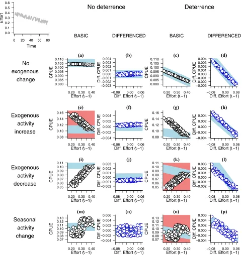
Figure 1. Basic (black circles) and differenced (blue circles) plots (defined in Table 1 footnote) of catch per unit effort (CPUE) against patrol effort in simulated patrol detections of poaching activity under decreasing effort in 8 scenario combinations of deterrence of poaching and exogenous change in poaching activity (n=80 and t is 1–80 in each graph). The graph with no letter label in the top-left shows the effort profile used in the simulations. The blue lines represent the shape of an ideal plot for distinguishing between the presence and absence of
plot of CPUEt against effortt−1 and the second is the
plot of differenced CPUE (CPUEt − CPUEt−1) against
differenced effort (effortt−1−effortt−2).
The default time lag in response by poachers to changes in ranger effort was equivalent to 1 time step. However, we also explored a more realistic scenario where we assumed imperfect knowledge of these lags and therefore compared CPUE with average patrol effort calculated over a moving window of time steps (q). For these simulations, effortt was recalculated as the mean of effortt−(q−1): effortt. In default simulations, q = 5. The resultant plots are hereafter referred to as MA (i.e., moving average) plots to contrast with the default (t−1) plots. We also considered the influences of temporal persistence of individual illegal activities between multiple time steps by repeating simulations for different (nonzero) values ofp.
In the presence of deterrence, we expected ideal plots to show a negative correlation, indicating that the rate of appearance of illegal activities decreased as patrol ef-fort increased; where deterrence was absent, the slope should be 0, since the frequency of illegal activities was independent of effort. The value of the slope under de-terrence can be calculated (Supporting Information), and we present these ideal values alongside the results. The higher ther2value, the more reliable the diagnostic. We appraised the 2 metrics according to these criteria.
Sensitivity Analyses
We repeated simulations for different values ofβ andγ, increasing and decreasing each by 10%. We also repeated simulations with greater amplitude of variation (CV = 0.19, 0.28, and 0.25 for stable, increasing, and decreasing profiles, respectively) to assess its impact on CPUE-effort relationships. The impact ofq, the width of the window of moving average, was assessed with differenced plots. The range of variation found in our estimates of δ in the few published studies available meant that we ran simulations for the full range to assess its impact.
All modeling and analyses were conducted using R software, version 3.2.3 (R Core Team 2017).
Results
Differenced (t − 1) plots consistently returned a clear negative correlation when deterrence was present and a slope close to 0 when it was absent, regardless of the presence or absence of exogenous changes in the appear-ance of illegal activities, across all effort profiles (Fig. 1 & Table 1). Basic plots yielded at least 1 diagnosis error in each effort profile and yielded far greater variation in both r2values and slope than differenced plots (Fig. 2a and c). Differenced MA plots were less reliable than differenced
0.0 0.2 0.4 0.6 0.8 1.0
0.0 0.2 0.4 0.6 0.8 1.0
Bas. Dif. Bas. Dif.
r
2
(
t
−1) plots
No Deterr. deterr.
(a)
0.0 0.2 0.4 0.6 0.8 1.0
0.0 0.2 0.4 0.6 0.8 1.0
Bas. Dif. Bas. Dif.
r
2
MA plots
No Deterr. deterr.
(b)
●
● ●
● −0.2
−0.1 0.0 0.1
0.2 ●
● ●
● −0.2
−0.1 0.0 0.1 0.2
Bas. Bas.
Slope
No Deterr. deterr.
(c)
●
● ●
● −0.2
−0.1 0.0 0.1 0.2
0.3 ●
● ●
● −0.2
−0.1 0.0 0.1 0.2 0.3
Bas. Bas.
Slope
No Deterr. deterr.
[image:7.594.311.535.53.315.2](d)
Figure 2. Parameters from basic (black circles and rectangles) and differenced (blue circles and
rectangles) plots (defined in Table 1 footnote) of catch per unit effort (CPUE) against patrol effort in
simulated patrol detections of poaching activity: (a, c) t−1 plots, poaching activity at time t is plotted against patrol effort at t−1; (b, d) MA plots, poaching activity at time t is plotted against the average patrol effort in the previous 5 time steps (Bas., basic plots; Dif., differenced plots; no deterr., no deterrence; deterr., deterrence present). In (a) and (b) r2values are from CPUE-effort plots across all combinations of patrol effort profile and exogenous change in
poaching activity (n=12 for each x-axis category) with and without deterrence of poaching (whiskers, lowest point within 1.5 interquartile ranges of the lower quartile and highest point within 1.5
interquartile ranges of the upper quartile). In (c) and (d) slope is of CPUE-effort (green line, ideal values: 0 slope when deterrence is absent [left side of each graph] and negative slope when deterrence is present [right side]). Calculations used to determine the ideal slope are in Supporting Information.
(t − 1) plots for identifying deterrence (compare r2, Fig. 2a and b), but the slopes were consistently informative in differenced MA plots and widely variable (hence unreliable) in basic MA plots (Fig. 2d).
Table 1. Mean slope andr2values for basic (CPUE-E) and differenced (CPUE-E) plotsaof illegal activities detected per unit of patrol effort (CPUE) against patrol effort in simulated patrol detections of poaching activity from the 12 scenario combinations of patrol effort profile and exogenous change in poaching.
Deterrence No deterrence
Plot type Effort typeb slope (SD) r2(SD) slope (SD) r2(SD)
Basic (CPUE-E) t−1 −0.06 (0.14) 0.59 (0.4) −0.01 (0.17) 0.47 (0.36) MA −0.06 (0.18) 0.56 (0.42) −0.02 (0.21) 0.55 (0.42) Differenced (CPUE-E) t−1 −0.05 (0.01) 0.89 (0.16) 0 (0) 0.08 (0.05) MA −0.07 (0.02) 0.1 (0.01) 0.01 (0.01) 0.16 (0.1)
aBasic plots are plots of CPUE over patrol effort. Differenced plots are plots of differenced CPUE (CPUE
t−CPUEt−1) over differenced patrol effort (effortt−1t−1 effortt−2).
bThe t−1 plots are those wherein CPUE (or differenced CPUE) at time t is plotted against patrol effort (or differenced effort) at time t−1. The MA plots are those wherein CPUE (or differenced CPUE) at time t is plotted against the average patrol effort (or differenced effort) across time steps t−4:t.
the individual outputs, such as Fig. 1, where graphs (b), (f), and (j) each appear to show an r2 approaching 1 because they were plotted with the same y-axis limits as graphs (d), (h), and (l) to allow slopes to be compared between deterrence and its absence. This may appear to undermine the superiority of the differenced plots, but an easy rule-of-thumb decision can be made: if there is a clear negative slope, deterrence may be operating, and, if not, deterrence is unlikely. No equivalent rule can be formulated for basic plots.
Increasing persistence in the detectability of illegal activities steadily reducedr2 values in differenced plots (basic plots were not tested) and reduced the steepness of the slope when deterrence was present (Fig. 3 & Table 2), thereby diminishing the ability of the plots to distinguish between the presence and absence of deterrence. This occurred via a simple mechanism. When activities persisted, changes in effort had impacts beyond the consecutive time step, blurring the relationship between effortt and CPUEt+1 where a relationship
was present and adding random noise where it was absent.
A related mechanism explains the fact thatr2values of the differenced plots diminished as the width of the win-dow, q, for calculating the moving average in MA plots increased from 1 to 4 (Supporting Information); random noise was introduced by the averaging of additional time steps that actually had no predictive value. Sensitivity tests revealed no meaningful influence of changes inβor γ, or of increased variance in effort profiles, on the rel-ative or absolute performances of basic and differenced t−1 plots, though greater amplitude did cause a slight increase inr2of differenced MA plots, as well as a more negative slope when deterrence was present (Supporting Information). The performance of differenced plots was insensitive to the maximum value ofδ, the total number of snares detected by all patrols per time step as a fraction of those present in the whole area atEmax(Dt/At); however, interpretation of the differenced plots was easiest for valuesδࣘ0.06. Asδincreased, both the ideal and realised slopes tended toward 0 (i.e., became less negative) under
deterrence, making deterrence progressively less clearly identifiable (Supporting Information).
The threshold of 0.06 is a practical rule of thumb as opposed to an essential criterion but, if applied, will effectively impose a constraint on the ratio of time-step length to patrol effort per time step (for a given detection rate). In the model, the value ofδwas set with reference to the absolute values of E, but when applying the method to real data, the patrol effort will be a known value, meaning that it is the length of the time step that must be deliberately chosen (Supporting Information).
Discussion
Deterrence is a fundamental aim of conservation law-enforcement patrols, but it is difficult to identify, such that very few convincing analyses exist that demonstrate deterrence empirically in the field (but see Moore et al. 2018). Observed declines in CPUE over time, which are frequently taken as evidence of deterrence, may be caused by exogenous processes that have little or nothing to do with behavioral responses to patrol effort. Here we demonstrate that basic CPUE-effort plots, which are often presented as a remedy to this issue, are vulnerable to the same forms of bias, and we show how differenced plots (CPUE-E) are more informative. Differenced plots reliably distinguished between the presence and absence of deterrence, regardless of the temporal distribution of effort or any exogenous change in illegal activity levels. These plots are no more conceptually complicated than the basic CPUE-effort plots and require no specialist knowledge or software to produce.
●
●
●
● ●
●
●
● ●
●
●
●
●
●
●●
●
●
●
●●● ●
●
●
●
●
● ● ●
●
● ●
●
●
●
●●
● ●
●● ●
●●
●
●
●
●
●
●
●
●
●
●
●
●
●
●
●
●
● ●
●● ●
●
●
●
●
●
●
●
●
●
●
●
●
−0.06 0.00 0.06 −0.01
0.00 0.01 0.02 0.03 0.04 0.05 0.06
● ●
● ●
● ●
● ● ● ● ● ● ●●●
● ●
● ● ● ● ● ●
● ● ●
● ●
●
● ●
●
● ●
● ● ●
● ● ● ●●● ●● ●●● ●
●
● ●
● ● ●
●
● ●
●●●● ●●●●●● ●●●● ●●●●●
Diff
. CPUE
Diff. Effort (t−1)
(a)
Persistence = 0●
●
● ●
●
●
● ●
●
●
●
●
●
●●
●
●
●
●●● ●
●
●
●
●
● ● ●
●
● ●
●
●
●
●●
● ●
●● ●
●●
●
●
●
●
●
●
●
●
●
●
●
●
●
●
●
●
● ●
●● ●
●
●
●
●
●
●
●
●
●
●
●
●
−0.06 0.00 0.06 −0.01
0.00 0.01 0.02 0.03 0.04 0.05 0.06
● ●
● ●
● ●
● ● ● ● ● ● ●●● ●●● ●●●● ●●●● ● ● ●●●●● ●
● ● ●
● ● ● ●●● ●● ●●● ●● ●●●● ●
●
● ●
●●●● ●●●●●● ●●●● ●●●●●
Diff. Effort (t−1)
(b)
Persistence = 0.3●
●
● ●
●
●
● ●
●
●
●
●
●
●●
●
●
●
●●● ●
●
●
●
●
● ● ●
●
● ●
●
●
●
●●
● ●
●● ●
●●
●
●
●
●
●
●
●
●
●
●
●
●
●
●
●
●
● ●
●● ●
●
●
●
●
●
●
●
●
●
●
●
●
−0.06 0.00 0.06 −0.01
0.00 0.01 0.02 0.03 0.04 0.05 0.06
● ●
● ●
●
● ●
● ● ● ● ●
●● ● ●●● ●●● ●●●
● ● ● ● ●● ●●
● ● ● ● ●●● ●● ●●●●●●● ●● ●●●● ●
●
● ●
●●●● ●●●●●● ●●●● ●●●●●
Diff. Effort (t−1)
(c)
Persistence = 0.6●
●
● ●
●
●
● ●
●
●
●
●
●
●●
●
●
●
●●● ●
●
●
●
●
● ● ●
●
● ●
●
●
●
●●
● ●
●● ●
●●
●
●
●
●
●
●
●
●
●
●
●
●
●
●
●
●
● ●
●● ●
●
●
●
●
●
●
●
●
●
●
●
●
−0.06 0.00 0.06 −0.01
0.00 0.01 0.02 0.03 0.04 0.05 0.06
● ● ●
● ● ●
● ● ● ● ● ●
● ● ●
● ●
● ● ● ● ● ●
● ● ● ● ● ●● ●●
● ●
● ● ●
● ● ● ●● ●●
● ● ● ● ●● ●●●●● ●●● ●●●● ●●●●●● ●●●● ●●●●●
[image:9.594.101.494.53.186.2]Diff. Effort (t−1)
(d)
Persistence = 0.9Figure 3. Impact of the persistence of evidence of poaching activity on differenced plots (defined in Table 1 footnote) of catch per unit effort (CPUE) against patrol effort in simulated patrol detections of poaching activity (n=80; t is 1–80). The scenario is deterrence of poaching with concurrent exogenous decline in poaching activity under the stable patrol-effort profile. Graph (a) is equivalent to graph (l) in Fig. 1. The equivalent plots without deterrence and plots with other combinations of exogenous change and effort profile are in Supporting
Information.
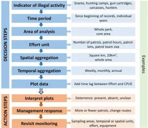
Figure 4. Decisions involved in
generating differenced plots (defined in Table 1 footnote) of catch per unit effort (CPUE) over patrol effort from basic antipoacher patrol data and
management actions taken as a result.
period to compensate for a potential lack of this knowl-edge, the plots became much noisier, though they could still be used to distinguish between deterrence and its absence.
Time lags are difficult to specify, given the current state of our understanding of the relationship between enforcement effort and illegal behavior. In the absence of independent data, it might be appropriate under some circumstances to make numerous plots, each at different time lags, and appraise all of them for signals of deter-rence, but there is a danger of data-mining and produc-ing spurious positive results by chance. We recommend choosing a small set of plausible potential time lags to
explore, based on poacher interviews, expert judgement or other lines of available evidence.
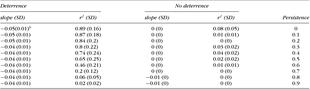
[image:9.594.42.344.277.539.2]Table 2. Mean slope andr2values for differenced plots (CPUE-E)aof illegal activities detected per unit of patrol effort (CPUE) against patrol effort in simulated patrol detections of poaching activity from the 12 scenario combinations of patrol effort profile and exogenous change in poaching under varying persistence times for evidence of poaching.
Deterrence No deterrence
slope (SD) r2(SD) slope (SD) r2(SD) Persistence
−0.05(0.01)b 0.89 (0.16) 0 (0) 0.08 (0.05) 0
−0.05 (0.01) 0.87 (0.18) 0 (0) 0.01 (0.01) 0.1
−0.05 (0.01) 0.84 (0.2) 0 (0) 0 (0) 0.2
−0.04 (0.01) 0.8 (0.22) 0 (0) 0.03 (0.02) 0.3
−0.04 (0.01) 0.74 (0.24) 0 (0) 0.04 (0.02) 0.4
−0.04 (0.01) 0.65 (0.25) 0 (0) 0.02 (0.02) 0.5
−0.04 (0.01) 0.46 (0.21) 0 (0) 0.01 (0.01) 0.6
−0.04 (0.01) 0.2 (0.12) 0 (0) 0 (0) 0.7
−0.04 (0.01) 0.06 (0.05) −0.01 (0) 0 (0) 0.8
−0.04 (0.01) 0.02 (0.02) −0.01 (0) 0 (0) 0.9
aDefinitions in Table 1 footnotes.
bThe first row is equivalent to row 3 of Table 1.
persistence may be an easier problem to manage than un-known time lags. The potential solutions are to conduct field experiments to determine how long various signs of illegal activity—from snares and gun cartridges to animal carcasses—remain detectable (fairly simple experiments may suffice) and to aggregate patrol data only across classes of activity that have similar persistence times.
A further complication, not addressed here, is that of spatial displacement. In the context of PA management, 3 broad outcomes of such displacement are possible. First, displacement occurs within the PA (no net reduction in illegal hunting). Second, displacement occurs from the entirety of the PA into surrounding areas of similar, unprotected habitat (hunting pressure may not be reduced). Third, displacement occurs from the entirety of the PA into surroundings that are unsuitable for hunting of the species of concern, but may still be good for other resource uses (displacement effectively constitutes a cessation of conservation-relevant hunting [i.e., deterrence]). In practice, the second and third outcomes are indistinguishable when no data from outside the PA are available, and the first outcome may not be obvious unless patrols include sufficient variety in their routes (Watson et al. 2013; Critchlow et al. 2015). Investigation of this phenomenon requires a spatially explicit model, ideally with individual agents representing patrols and potential offenders, and programmed responses linking enforcement effort with behavior of the latter. The spatial unit over which data are aggregated must also be considered in light of displacement; where fine-scale information is lacking, the PA boundary is probably the most parsimonious choice.
There are also factors we did not consider, such as vari-ation in patrol motivvari-ation and efficiency, that could either mask or mimic a signal of deterrence, and that merit investigation. The effects of deterrence and other aspects of law enforcement on hunter behavior are also likely to be dependent upon the socioeconomic circumstances