Volume 2, No. 6, Nov-Dec 2011
International Journal of Advanced Research in Computer Science
RESEARCH PAPER
Available Online at www.ijarcs.info
410
Adaptive Rood Algorithm for Motion compensation in video streams
Sanipini Venkata Kiran*1, P. Darwin2
1,2
Department of ECE,
Godavari Institute of Engineering and Technology Rajahmundry, Andhra Pradesh, India
1
[email protected], [email protected]
Ch. Srinivasa Rao
Department of ECE,
Sri Sai Aditya Institute of Engineering and Technology Surampalem, Andhra Pradesh, India
Abstract— Video compression plays major role in multimedia industry in general. The rapid advances in the video compression algorithms aims at reducing redundancy without compromising the quality. A video captured was encoded using the encoder with each frame processed by dividing it into several motion-blocks. In the encoder part, several motion estimation algorithms were applied. The quality metric, Peak Signal to Noise Ratio (PSNR) for multiple frames was calculated for all available algorithms. From all these it is found that Adaptive Rood Pattern Search (ARPS) algorithm eliminates redundancy without compromising the image quality. This algorithm was used to generate the motion vectors to produce the compensated image, and this image was transformed using Discrete Cosine Transform (DCT) then quantized and encoded in the encoder. For achieving better PSNR and to reduce the number of search points required to generate the motion vector ARPS algorithm is proved superior when compared to the other available searching algorithms.
Keywords - Adaptive Rood Pattern Search (ARPS), Discrete Cosine Transform (DCT), Peak Signal to Noise Ratio (PSNR), Motion compensation.
I. INTRODUCTION
With the advent of the multimedia age and the spread of internet, video storage on CD/DVD and streaming of video has been gaining a lot of popularity. Video compression becomes a direct need as video usage on the internet growing day by day. So, video compressions address this problem by exploiting spatial and temporal redundancy. In spatial redundancy, redundancy is reduced by considering neighboring samples on a scanning line that are generally similar. In digital video, in addition to spatial redundancy, neighboring frames in a video sequence may be similar (temporal redundancy).
Motion compensation is a predictive technique for exploiting the temporal redundancy between successive frames of video sequence. Motion estimation is a technique to eliminate temporal redundancy of image sequences and it is the central part of the Moving Pictures Expert Group (MPEG (1/2/4)) [1-3] and the video compression standards (H.261/H.263) [4]. However, motion estimation involves a lot of computational complexity in the video encoders and it occupies not less than 70-75 percent of the entire processing time of a video coder.
Motion estimation is the process of determining motion vectors that describe the transformation from one 2D image to another, usually from adjacent frames in a video sequence. It is an ill-posed problem as the motion is in three dimensions but the images are projections of the 3D scene onto a 2D plane. The motion vectors may relate to the whole image (global motion estimation) or specific parts, such as rectangular blocks, arbitrary shaped patches or even per pixel. The motion vectors may be represented by a translational model or many other models that can approximate the motion of a real video camera, such as rotation and translation in all three dimensions. Optical flow reflects the image changes due to changes in motion during a small time gap. Optical flow field is the velocity field that represents the 3D motion of object points across a 2D image. It should not be sensitive to illumination changes and motion of unimportant objects. The optical flow field is
represented in the form of velocity vector. The length, direction of this vector determines the magnitude of velocity and the direction of motion. The optical flow can be computed either globally or locally. In global flow estimation local constraints are propagated globally but the disadvantage is errors also propagate across the solution. In local flow the image is divided into smaller regions but it is inefficient in the areas where spatial gradients change slowly and in that case use global approach.
This paper is organized as follows. A detailed review of various motion estimation algorithms available in the current literature is presented in section 2. Proposed Adaptive rood algorithm is discussed in section 3. Results and discussion is presented in section 4. Conclusions are given in section 5.
II.RELATEDWORK
411
Figure.1 Forward and backward motion estimation.
We consider the estimation of motion between two given frames, the MV at x between time t1 and t2 is defined as the displacement of this point from t1 to t2.We will call the frame at time t1 anchor frame and the frame at t2 tracked frame. Depending on the intended application the tracked frame can be either before or after the tracked frame in time. As illustrated in Fig.1 the problem is referred to as forward motion estimation, when t1<t2, and as backward motion estimation, when t1>t2. For example in this paper we use Rhinos video sequence which uses forward motion estimation has anchor frame and a tracked frame as shown in Fig.2.
There are two mainstream techniques of motion estimation: pel-recursive algorithm (PRA) [5] and block-matching algorithm (BMA). PRAs are iterative refining of motion estimation for individual pels by gradient methods. BMAs assume that all the pels within a block has the same motion activity[10]. BMAs estimate motion on the basis of rectangular blocks and produce one motion vector for each block. PRAs involve more computational complexity and less regularity.
Frame (1) Frame (2)
(Anchor frame) (Tracked frame)
Figure.2 Anchor and tracked frames of Rhino video sequence.
The underlying supposition behind motion estimation is that the patterns corresponding to objects and background in a frame of video sequence move within the frame to form corresponding objects on the subsequent frame. The idea behind block matching is to divide the current frame into matrix of ‗macro blocks‘ (MB) that are then compared with corresponding block and its adjacent neighbors in the previous frame to create a vector that stipulates the movement of a macro block from one location to another in the previous frame. This movement calculated for all the
macro blocks comprising a frame, constitutes the motion estimated in the current frame. The search area for a good macro block match is constrained up to p pixels on all fours sides of the corresponding macro block in previous frame.
This ‗p‘ is called as the search parameter. Larger motions
require a larger p, and the larger the search parameter the more computationally expensive the process of motion estimation becomes. Usually the macro block is taken as a square of side 16 pixels, and the search parameter p is 7 pixels. The idea is represented in Fig 3.
Figure.3 Motion estimation and motion vector
The matching of one macro block with another is based on the output of a cost function. The macro block that results in the least cost is the one that matches the closest to current block. There are various cost functions, of which the most popular and less computationally expensive is Mean Absolute Difference (MAD) given by equation
1 1
2 1 1
1
|
|
N N
ij ij i j
MAD
C
R
N
Another cost function is Mean Squared Error (MSE) given by equation
1 1
2 2
1 1
1
(
)
N N
ij ij i j
MSE
C
R
N
Where N is the side of the macro bock, Cij and Rij are the
Pixels being compared in current macro block and reference macro block, respectively.
Peak-Signal-to-Noise-Ratio (PSNR) given by the below equation characterizes the motion compensated image that is created by using motion vectors and macro blocks from the reference frame.
2 10
(Peak to peak value of original signal)
10 log [ ]
PSNR
MSE
There are various algorithms that have been implemented so far are Full Search (FS), Three Step Search (TSS), Simple and Efficient TSS (SES), New Three Step Search (NTSS), Four Step Search (SS4), Diamond Search (DS). These are discussed briefly in this section.
A. Full Search (FS):
412 Fast block matching algorithms try to get the same PSNR
doing little computations.
B. Three Step Search (TSS):
This is one of the earliest attempts at fast block matching algorithms. The general idea is represented in Fig 4. It starts with the search location at the center and sets the ‗step size‘ S = 4, for a usual search parameter value of 7. It then searches at eight locations +/- S pixels around location (0, 0). From these nine locations searched so far it picks the one giving least cost and makes it the new search origin. It then sets the new step size S = S/2, and repeats similar search for two more iterations until S = 1. At that point it finds the location with the least cost function and the macro block at that location is the best match. The calculated motion vector is then saved for transmission. It gives a flat reduction in computation by a factor of 9. So that for p = 7, ES will compute cost for 225 macro blocks whereas TSS computes cost for 25 macro blocks [11].
Figure.4 The Three Step Search Procedure
The idea behind TSS is that the error surface due to motion in every macro block is unimodal. A unimodal surface is a bowl shaped surface such that the weights generated by the cost function increase monotonically from the global minimum.
Fig.5 Search patterns corresponding to each selected quadrant: (a) Shows all quadrants (b) quadrant I is selected (c) quadrant II is selected (d)
quadrant III is selected (e) quadrant IV is selected.
C. Simple and Efficient Search (SES):
SES [6] is another extension to TSS and exploits the assumption of unimodal error surface. The main idea behind the algorithm is that for a unimodal surface there cannot be two minimums in opposite directions and hence the 8 point fixed pattern search of TSS can be changed to incorporate this and save on computations.
The algorithm still has three steps like TSS, but the innovation is that each step has further two phases. The search area is divided into four quadrants and the algorithm checks three locations A, B and C as shown in Figure 5. A is at the origin and B and C are S = 4 locations away from A in orthogonal directions. Depending on certain weight distribution amongst the three the second phase selects few additional points (Fig 5). The rule for determining a search quadrant for seconds phase is as follows:
If MAD A MAD B and MAD A MAD C ,select b ;
If MAD A MAD B and MAD A MAD C ,select c ;
If MAD A <MAD B and MAD A < MAD C ,select d ;
If MAD A <MAD B and MAD A MAD C ,select e ;
Figure.6 The SES procedure. The motion vector is (3, 7).
Once we have selected the points to check for in second phase, we find the location with the lowest weight and set it as the origin. We then change the step size similar to TSS and repeat the above SES procedure again until we reach = 1.The location with the lowest weight is then noted down in terms of motion vectors and transmitted. An example process is illustrated in Fig 6.Although this algorithm saves a lot on computation as compared to TSS, it was not widely accepted for two reasons. Firstly, in reality the error surfaces are not strictly unimodal and hence the PSNR achieved is poor compared to TSS. Secondly, there was another algorithm, Four Step Search, that presentes low computational cost compared to TSS and gave significantly better PSNR.
D. New Three Step Search (NTSS):
413 NTSS process is illustrated graphically in Fig 7. In the first
[image:4.595.43.270.267.456.2]step 16 points are checked in addition to the search origin for lowest weight using a cost function. Of these additional search locations, 8 are a distance of S = 4 away (similar to TSS) and the other 8 are at S = 1 away from the search origin. If the lowest cost is at the origin then the search is stopped right here and the motion vector is set as (0, 0). If the lowest weight is at any one of the 8 locations at S = 1, then we change the origin of the search to that point and check for weights adjacent to it. Depending on which point it is we might end up checking 5 points or 3 points. The location that gives the lowest weight is the closest match and motion vector is set to that location. On the other hand if the lowest weight after the first step was one of the 8 locations at S = 4, then we follow the normal TSS procedure. Hence although this process might need a minimum of 17 points to check every macro block, it also has the worst-case scenario of 33 locations to check.
Figure.7 New Three Step Search block matching
E. Four Step Search (4SS):
[image:4.595.317.556.446.661.2]Similar to NTSS, 4SS [8] also employs center biased searching and has a halfway stop provision. 4SS sets a fixed pattern size of S = 2 for the first step, no matter what the search parameter p value is. Thus it looks at 9 locations in a 5x5 window. If the least weight is found at the center of search window the search jumps to fourth step. If the least weight is at one of the eight locations except the center, then we make it the search origin and move to the second step. The search window is still maintained as 5x5 pixels wide.
Figure.8 Four Step Search procedure. The motion vector is (3,-7).
Depending on where the least weight location was, we might end up checking weights at 3 locations or 5 locations. The patterns are shown in Fig 8. Once again if the least weight location is at the center of the 5x5 search window we jump to fourth step or else we move on to third step. The third is exactly the same as the second step. In the fourth step the window size is dropped to 3x3, i.e. S = 1. The location with the least weight is the best matching macro block and the motion vector is set to point at that location. A sample procedure is shown in Fig 8. This search algorithm has the best case of 17 checking points and worst case of 27 checking points.
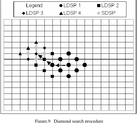
F. Diamond Search (DS):
Diamond search (DS) algorithm is exactly the same as 4SS, but the search point pattern is changed from a square to a diamond, and there is no limit on the number of steps that the algorithm can take.DS uses two different types of fixed patterns, one is Large Diamond Search Pattern (LDSP)[14] and the other is Small Diamond Search Pattern (SDSP). These two patterns and the DS procedure are illustrated in Fig. 9. Just like in FSS, the first step uses LDSP and if the least weight is at the center location e jump to fourth step. The consequent steps, except the last step, are also similar and use LDSP, but the number of points where cost function is checked are either 3 or 5 and are illustrated in second and third steps of procedure shown in Fig.9.
The last step uses SDSP around the new search origin and the location with the least weight is the best match. As the search pattern is neither too small nor too big and the fact that there is no limit to the number of steps, this algorithm can find global minimum very accurately. The end result should see a PSNR close to that of ES while computational expense should be significantly less.
Figure.9 Diamond search procedure
III. PROPOSED ADAPTIVE ROOD
ALGORITHM
[image:4.595.42.273.597.773.2]414 can easily detect the large motions but they tend to go for
unnecessary searches when detecting the small motions. Hence it is desirable to use different search patterns according to the estimated motion behavior (in terms of the magnitude of motion) for the current block. This boils down to two issues required to be addressed: 1) How to predetermine the motion behavior of the current block for performing efficient motion estimation? and 2) what is the most suitable size and the shape of the search pattern(s).
Regarding the first issue, in most cases adjacent MBs belonging to the same moving object have similar motions. Therefore the motion vector for the current MB can be reasonably predicted from the neighboring MB‘s motion vectors in the spatial or temporal domains. As for the second issue two types of search patterns are used. One is Adaptive Rood Pattern (ARP) with adjustable rood arm, which is dynamically determined for each MB according to the predicted motion behavior. Note that the ARP will be exploited only once in the beginning of the MB search. The objective is to find a good starting point for the remaining local search so as to avoid unnecessary intermediate search and reduce the risk of being trapped into the local minimum in case of long search path. The starting point identified is hopefully as close as to the global minimum as possible. If so then, a small fixed size search pattern will be able to complete the remaining local search quickly.
Note also that this small search pattern will be used repeatedly unrestrictedly until the final MV is found.
A. Prediction of the Target MV:
In order to obtain the accurate MV prediction of the current block two factors need to be considered: 1) Choice of the Region of Support (ROS) that consists of the neighboring
Blocks whose MVs are used to calculate the predicted MV, and 2) algorithm used to construct the predicted MV.
In the temporal region the block in the reference frame at the same position as that of current block in the present frame is a straight forward choice as a temporal ROS candidate. However, the neighboring blocks from the same reference frame can also be used for prediction. However there would be a large requirement of memory if such a kind of operation is performed, as the MV information of the complete reference frame should be stored. So the choice of temporal prediction will be eliminated due to the huge memory requirement and computations.
The other way possible is to go for the spatial prediction. Usage of the already calculated i.e. the neighboring blocks MVs as a source for prediction will be a good option. It is the only possible way to have less memory requirement. The concept of Region of Support (ROS) is used for the prediction of current block MV. There are 4 kinds of ROS possible. They are as follows.
TYPE A TYPE B TYPE C TYPE D
Figure.10 Types Of Region of Supports [16]
TYPE A ROS covers all the four neighboring blocks and TYPE B is the prediction ROS that is adopted in some international standards such as H.263 for the differential coding of the MVs. TYPE C composed of the two directly adjacent blocks, TYPE D consists of only one adjacent block that is left of the current MB. Experiments on various types of ROCs is being done and it was observed that they yield fairly similar results with a difference of less than 0.1 DB in PSNR and 5% in the number of search points. Hence it is wise to choose TYPE D kind of ROS hence it requires only one motion vector for prediction.
B. Selection of Search Patterns:
For initial Search: The shape of the rood pattern is symmetrical that is shown in the Fig 11.The main structure of ARP takes the rood shape, its size refers to the distance between center point and the any of the other vertex point. The shape of the rood pattern is determined on the basis of real world motion sequences. For most of the sequences it was observed that the motion vector distribution was mostly in horizontal and vertical direction than in other directions, since the camera movements are mostly in those directions. Since the rood pattern spreads in both the vertical and horizontal directions it can quickly detect the motion vectors and also can able to jump directly into the local region of the global minimum. Secondly, any MV can be decomposed into one vertical MV component and one horizontal MV component. For a moving object which may introduce motion in any direction the rood shaped pattern can atleast detect the major trend of the moving object which is the desired outcome of the initial search stage.
In addition to the four search points it would be better to include the position of the predicted motion vector that aids in the termination in the initial search stage only if the predicted MV matches with the target MV. So in total there will be six search points in the initial search stage and then five search points for the further refinement process.The search pattern that will be used in the initial search stage is shown in the Fig.11.
Figure.11 Adaptive Rood Pattern: The predicted motion vector is (2,-1), and the step size S = Max (|2|, |-1|) = 2.
In this method the Rood Arm Length (RAL) will be equal to the and the four arms are of equal length. Mathematically it can be expressed as follows.
415
Ѓ is = Round (MV predicted)
=Round ( MV2predicted(x) + MV2predicted(y))
Where the MVpredicted(x) is the x-component of the
predicted motion vector and the MVpredicted(y) is the
y-component of the predicted motion vector. Operator Round performs the rounding operation to the nearest possible integer since the displacement can be in terms of the integers.
It should be kept in mind that the TYPE D kind of ROS cannot be used for all MBs, because there will be some MBs where there will be no left neighbor.
So, in that case the ARP with RAL of 2 (Ѓ = 2) is suggested, by taking the reference of LDSP, which has fairly a good amount of performance. Also larger MVs are not preferred as the boundary MVs mostly belong to the static background, which do not contribute larger MVs.
C. Fixed Pattern:
For Refined Local Search: In the initial search the adaptive rood pattern directly leads to the new search position which is somewhere around global minimum, which avoids the unnecessary search points in the intermediary search path. Since there is no chance of getting trapped into the local minimum we can use the fixed pattern for identifying the global minimum. The minimum error point in the first step is used to align as the centre of the fixed pattern in the second step. This process will be followed until the point of minimum error is the centre of the present iteration‘s search pattern.
Two types of fixed patterns were proposed. The first one was the 3x3 square patterns as was proposed in the SDSP. The second pattern consists of a unit size rood arm pattern.
The experimental results conducted by [16] showed that the 3x3 square pattern yields similar PSNR when compared to the Unit rood arm pattern but 40% to 80% more number of search points. This demonstrates the efficiency of the Unit Rood Arm Pattern. The proposed fixed patterns by [16] are shown in the figure 12.
Figure.12 Fixed size Patterns [16]
D. Proposed ARPS Algorithm:
Step 1:- Compute the matching error (SAD centre) between
the current block and the block at the same location in the reference frame (i.e. centre of the current search window). If the current block is the left most Ѓ = 2;
Else
Ѓ =Max (|MVpredicted(x) |,| MVpredicted(y)|)
Go to step 2
Step 2:- Align the centre of ARP with the centre point of the search window and check its 4points and the position of the predicted motion vector to find the minimum error point.
Step3:- Set the centre point of the unit size rood pattern at the minimum error point found in the previous step and check its points. If the new minimum error point is not incurred at the centre of the unit rood pattern repeat this step otherwise, MV is found corresponding to the minimum error point in the current step.
ARPS algorithm makes use of the fact that the general motion in a frame is usually coherent, i.e. if the macro blocks around the current macro block moved in a particular direction then there is a high probability that the current macro block will also have a similar motion vector[16]. This algorithm uses the motion vector of the macro block to its immediate left to predict its own motion vector. An example is shown in Fig.11, the predicted motion vector points to (2, -1). In addition to checking the location pointed by the predicted motion vector, it also checks at a rood pattern distributed points, as shown in Fig 11, where they are at a step size of S = Max (|X|, |Y|). X and Y are the x-coordinate and y-coordinate of the predicted motion vector. This rood pattern search is always the first step.
It directly keeps the search in an area where there is a high probability of finding a good matching block. The point that has the least weight becomes the origin for subsequent search steps, and the search pattern is changed to SDSP.
The procedure keeps on doing SDSP until least weighted point is found to be at the center of the SDSP. A further small improvement in the algorithm can be to check for Zero Motion Prejudgment [8], using which the search is stopped half way if the least weighted point is already at the center of the rood pattern.
Care also needs to be taken when the predicted motion vector turns out to match one of the rood pattern location. We have to avoid double computation at that point. For macro blocks in the first column of the frame, rood pattern step size is fixed at 2 pixels.
IV. SIMULATION RESULTS
The efficiency of the proposed algorithm was tested by using two benchmark video sequences, Rhinos and
Vipmosaicking.Consecutive 70 frames of size 320 240
pixels in Rhinos and consecutive 70 frames of size 320 240 pixels in Vipmosaicking are considered first. The block and search window sizes were fixed at 16 16 and 33 33 respectively.
416
Figure.13 PSNR performance of Fast Block Matching Algorithms. Rhinos Sequence was used with a frame distance of 2.
Figure.13 PSNR performance of Fast Block Matching Algorithms. Vipmosaicking Sequence was used with a frame distance of 2.
Figure.15 Number of computations of various algorithms compared with ARPS for Vipmosaicking sequence.
As is shown by Fig. 13, 4SS, DS and ARPS come pretty close to the PSNR results of ES. While the ES takes on an average around 225 searches per macro block, DS and 4SS drop that number by more than an order of magnitude of DS. NTSS and TSS although do not come close in PSNR performance to the results of ES, but even they drop down the number of computations required per macro block by almost an order of magnitude. SES takes up less number of search point computations amongst all but ARPS. However, it also has the worst PSNR performance. Although PSNR performance of 4SS, DS, and ARPS is relatively the same, ARPS takes a factor of 2 less computations and hence is the best of the fast block matching algorithms studied in this paper.
The main advantage of the ARPS algorithm over DS is that if the predicted motion vector is (0, 0), it does not waste computational time in doing LDSP; it rather directly starts using SDSP. Furthermore, if the predicted motion vector is far away from the center, then again ARPS save on computations by directly jumping to that vicinity and using SDSP, whereas DS takes its time doing LDSP.
Table.1 PSNR performance of various motion estimation algorithms along with Adaptive Rood Pattern Search, Rhinos Sequence was used with a frame distance of 2.
Frames ES_PSNR TSS_PSNR NTSS_PSNR SESTSS_PSNR SS4_PSNR DS_PSNR ARPS_PSNR
0 19.1816 18.9842 18.944 18.3745 18.7857 18.836 18.9487
10 29.0757 28.4340 28.4315 24.9953 27.1993 27.1861 27.3256
20 22.6957 22.5244 22.5086 21.4281 22.2785 22.1907 22.5721
30 19.9814 19.8862 19.8825 19.5873 19.7173 19.7276 19.8131
40 19.9239 19.8524 19.8512 19.445 19.7316 19.7428 19.8322
50 20.2241 20.1652 20.1516 19.7422 20.0569 20.0796 20.0396
60 21.8762 21.6787 21.6716 21.0378 21.6035 21.6521 21.7536
417
Table.2 PSNR performance of various motion estimation algorithms along with Adaptive Rood Pattern Search Vipmosaicking Sequence was used with a frame distance of 2.
Frames ES_PSNR TSS_PSNR NTSS_PSNR SESTSS_PSNR SS4_PSNR DS_PSNR ARPS_PSNR
0 26.1276 25.1085 25.1017 21.1807 24.4313 23.7763 25.298 10 25.4268 24.4815 24.1809 23.8878 24.435 24.556 25.3272 20 24.5511 24.0288 23.562 23.2236 23.969 23.922 24.2797 30 29.2803 28.491 27.4074 28.0707 28.9618 28.918 29.1483 40 32.4371 30.6876 28.5425 30.3112 28.1771 27.7556 32.1894 50 23.7483 23.3847 23.381 22.8618 23.1063 22.92 23.535 60 26.6763 25.2653 25.1849 25.8246 25.0706 25.1363 26.424 70 39.6937 39.7064 39.7064 39.6992 39.6935 39.7117 39.7102
V. CONCLUSIONS
The theory of all motion estimation algorithms are explored in this work and examined basic features of motion estimation algorithms. Even though more commonly linked to lossy video compression, motion estimation is infact a technique that goes beyond and allows for video processing and computational vision algorithms and applications.
It allows a computer to detect movement as well as to perform comprehensive video sequence analysis, identifying scenes, camera and object movements. Motion estimation is one technique that allows for a simple, yet effective, object identification scheme. Seven different algorithms for motion estimation are tested and compared average number of search points and PSNR. It is concluded that Adaptive Rood Pattern Search Algorithm gives better result compared to all other existing algorithms in terms of achieving best PSNR and it also reduces the number of search points required for generating the motion vector.
VI. REFERENCES
[1] MPEG, ―IS0 CD11172-2; Coding of moving pictures and associated audio for digital storage media at up to about 1.5 Mbits/s,” Nov. 1991.
[2] ISO/IEC 11 172-2 (MPEG-1 Video), ―Information
technology-Coding of moving pictures and associated audio for digital storage media at up to about 1.5 Mbit/s: Video,‖ 1993.
[3] ISO/IEC 13818-2 I ITU-T H.262 (MPEG-2 Video),
―Information technology- Generic coding of moving pictures and associated audio information: Video,‖ 1995.
[4] CCITT SGXV, ―Description of reference model 8 (RM8),‖ Document 525, Working Party XV/4, specialists Group on Coding for Visual Telephony, Jun. 1989.
[5] A. N. Netravali and J. D. Robbins, ―Motion compensated television coding: Part- I,‖ Bell Syst. Tech. J., vol. 58, pp. 631–670, Mar. 1979.
[6] Jianhua Lu, and Ming L. Liou, ―A Simple and Efficient Search Algorithm for Block-Matching Motion Estimation‖, IEEE Trans.Circuits And Systems For Video Technology, vol 7, no. 2, pp. 429-433,April 1997.
[7] Renxiang Li, Bing Zeng, and Ming L. Liou, ―A New Three-Step Search Algorithm for Block Motion Estimation‖, IEEE Trans. Circuits And Systems For Video Technology, vol 4., no. 4, pp. 438-442, August 1994.
[8] Jong-Nam Kim and Tae-Sun Choi, ―A Fast Three Step
Search Algorithm with Minimum Checking Points,‖ Proc. of IEEE conference on Consumer Electronics,
[9] pp.132-133, 2-4 June 1998.
[10]Lai-Man Po and Wing-Chung Ma, ―A Novel Four-Step Search Algorithm for Fast Block Motion Estimation‖, IEEE Transactions on Circuits and Systems for Video Technology, vol. 6, no. 3, pp.313-317, June 1996
[11]T. Koga, K. Iinuma, A. Hirano, Y. Iijima, and T. Ishiguro, ―Motion compensated interframe coding for video conferencing,‖ in Proc. Nat. Telecommun. Conf., New Orleans, LA, pp. G5.3.1– G5.3.5, Nov. 29–Dec. 3 1981. [12]Jong-Nam Kim and Tae-Sun Choi, ―A Fast Three Step
Search Algorithm with Minimum Checking Points,‖ Proc. of IEEE conference on Consumer Electronics, pp.132-133, 2-4 June 1998.
[13]Th. Zahariadis and D. Kalivas ―A Spiral Search Algorithm for Fast Estimation of Block Motion Vectors,‖ Signal Processing VIII, theories and applications. Proceedings of the EUSIPCO 96. Eighth European Signal Processing Conference p.3 vol. lxiii + 2144, vol. 2, pp. 1079-82, 1996.
[14] M.Porto, L.Agostini, S.Bampi and A.Susin, ―A high throughput and low cost diamond search architecture for HDTV Motion estimation,‖ IEEE International Conference on Multimedia and Expo 2008, pp.1033-1036, 2008.
[15]Shan Zhu, and Kai-Kuang Ma, ― A New Diamond
Search Algorithm for Fast Block-Matching Motion Estimation‖, IEEE Trans. ImageProcessing, vol 9, no. 2, pp. 287-290, February 2000.
[16]Y.Nie and K-k Ma, ―Adaptive Rood Pattern Search for fast block matching algorithms,‖ IEEE Trans. on Image Processing, vol 11, no. 12, pp.1442-1448,December 2002. [17]C.-H. Hsieh, P. C. Lu, J.-S. Shyn, and E.-H. Lu, ―Motion
estimation algorithm using interblock correlation,‖ Electron. Lett., vol. 26, no. 5, pp. 276–277, Mar. 1, 1990.
[18] K.K. Ma and G. Qiu, ―Adaptive Rood Pattern Search for Fast Block Matching Motion Estimation in JVT/H.26L,‖ IEEE International Conference on Image Processing 2003, pp. ii-708 – ii-711, 2003.
[19]J.-B. Xu, L.-M. Po, and C.-K. Cheng, ―Adaptive motion tracking block matching algorithms for video coding,‖ IEEE Trans. Circuits Syst. Video Technol., vol. 97, pp. 1025–1029, Oct. 1999.
[20]J. Chana and P. Agathoklis, ―Adaptive motion estimating for efficient video compression,‖ in Conf. Rec. 29th Asilomar Conf. Signals, Systemsand Computers, vol. 1, 1996, pp. 690– 693,1996.
[21]D.-W. Kim, J.-S. Choi, and J.-T. Kim, ―Adaptive motion estimation based on spatio–temporal correlation,‖ Signal Process.: ImageCommun. vol. 13, pp. 161–170, 1998.
418 Short Biodata for the Author
S. VenkataKiran is currently pursuing his
M.Tech degree from ECE Department of Godavari Institute of Engineering and Technology, Rajahmundry, AP, India. He has completed his B. Tech from Aditya Engineering College, Surampalem, AP, India.
P
. Darwin is currently working as Associate Professor of ECE Department in Godavari Institute of Engineering and Technology, Rajahmundry, AP, India .He received his M. Tech. degree from University College of Engineering, JNTUK, Kakinada, A.P, India. Hehas seventeen years of experience in teaching and industry.
Ch. Srinivasa Rao is currently working as