Routing Applications
Francesco Bertoli
A thesis submitted for the degree of
Doctor of Philosophy of
The Australian National University
I first wish to thank my primary supervisor: Phil. I guess it’s not easy to take in a Ph.D. student half way through his time. Especially if he moves to Sydney before starting to work with you. Thanks for the time you dedicated to me. In particular, I want to thank you for helping me find my way in the research world. Before turning my attention to OR, I was losing my interest in research.
A huge “thank you” goes to Tommaso. For many many reasons. First, because you helped me in my transition. Then for all your attention and dedication, and for being a real-time available library on programming. Last but not least, for hosting me pretty much every time I came to Canberra and for making those visits fun. I really enjoyed working together, and I hope we’ll have another chance.
I also wish to thank Adrian. If I came to Australia for my Ph.D., it was thanks to you. Moreover, I appreciated you following me every day while we were working together. I also appreciate the opportunity you gave me to visit and give seminars in several cool places.
I must, and want to, give thanks to my family. My parents, for being my parents and a limitless source of support. My brother, for being my brother. I cannot explain it a different way. Thanks for coming down to the other side of the world several times. It meant a lot and it made the distance shorter.
There are so many people that I have met during these four years that I want to remember and acknowledge. Enrico, Sara and Alessandro, for giving me an (Italian) place to stay in Canberra. I hope I’ll see you again back home. Antonio, Pierrick, Hannah and their cool housemates, and Andrei and Arthur, for their hospitality, which I appreciated very much. I had much fun staying with you guys. I really hope to meet again somewhere in the world. Alessandro, for making me discover the OR world. The Couchsurfing community in Canberra, you made it easy to move to a new continent. I don’t know what I would have done without the Tuesday meetings. The Awesome Kids, which I think is the nicest group of people I have ever met. Remy, Laura, David, Jackie, Mark for all the fun climbing together. Nick and Tracy, I can now say thanks for the trust. The Sydney crew, no need to say we will see each other
again. Finally, thanks to the Hivery team, for making me living a great experience.
The class of Vehicle Routing Problems (VRPs) is one the most studied topics in the Operations Research community. The vast majority of the published papers focus on single-period problems, with a few branches of the literature considering multi-period generalisations. All of these problems though, consider a short horizon and aim at optimising the decisions at an operational level, i.e. that will have to be taken in the near future. One step above are tactical problems, i.e. problems concerning a longer time horizon. Tactical problems are of a fundamental importance as they directly influence the daily operations, and therefore a part of the incurred costs, for a long time. The main focus of this thesis is to study tactical problems arising in routing applications.
The first problem considered concerns the design of a fleet of vehicles. Trans-portation providers often have to design a fleet that will be used for daily operations across a long-time span. Trucks used for transportation are very expensive to pur-chase, maintain or hire. On the other side, the composition of the fleet strongly influences the daily plans, and therefore costs such as fuel or drivers’ wages. Bal-ancing these two components is challenging, and optimisation models can lead to substantial savings or provide a useful basis for informed decisions
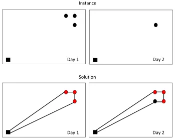
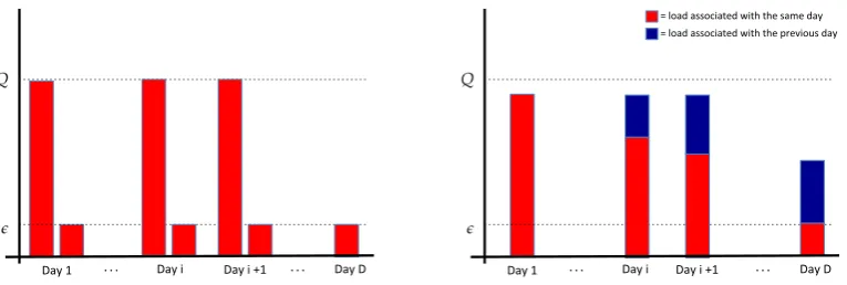
The second problem presented focuses on the use of a split deliveries policy in multi-period routing problems. It is known that the combined optimisation of deliv-ery scheduling and routing can be vdeliv-ery beneficial, and lead to significant reductions in costs. However, it also adds complexity to the model. The same is true when split deliveries are introduced. The problem studied considers the possibility of splitting the deliveries over different days. An analysis, both theoretical and numerical, of the impact of this approach on the overall cost is provided.
Finally, a districting problem for routing applications is considered. These types of problems typically arise when transportation providers wish to increase their service consistency. There are several reasons a company may wish to do so: to strengthen the customer-driver relationship, to increase drivers’ familiarity with their service area, or, to simplify the management of the service area. A typical approach, considered here, is to divide the area under consideration in sectors that will be subsequently assigned to specific drivers. This type of problem is inherently of a multi-period and tactical nature. A new formulation is proposed, integrating stand-ard routing models into the design of territories. This makes it possible to investigate
x
TSP Travelling Salesman Problem
VRP Vehicle Routing Problem
VRPTW Vehicle Routing Problem with Time Windows
CVRP Capacitated VRP
PVRP Periodic Vehicle Routing Problem
IRP Inventory Routing Problem
SDVRP Split Deliveries VRP
MDSDVRP Multi Day Split Deliveries VRP
FSM Fleet Size and Mix
DC Distribution Centre
TS Tabu Search
SA Simulated Annealing
LNS Large Neighborhood Search
ALNS Adaptive Large Neighborhood Search
CG Column Generation
TDP Territory Design Problems
TBR Territory Based Routing
Acknowledgments vii
Abstract ix
Glossary xi
1 Introduction xxi
1.1 Background and Motivation . . . xxi
1.2 Objectives and Contributions . . . xxiii
1.3 Uncertainty in Tactical Problems . . . xxv
1.4 Thesis Outline . . . xxvi
1.5 Notation . . . xxvii
I Mathematical Background 1 2 Routing Problems 3 2.1 The Vehicle Routing Problem . . . 3
2.2 Routing Problems . . . 4
2.2.1 Requests . . . 4
2.2.2 Routes . . . 5
2.2.3 Fleet . . . 6
2.2.4 Objectives . . . 7
2.3 Multi-Period Problems . . . 8
2.4 Tactical Routing Problems . . . 10
3 Solution Methods 11 3.1 Exact Methods . . . 11
3.1.1 Set Partitioning Formulations . . . 13
3.2 Column Generation . . . 14
3.2.1 Common Issues . . . 16
3.2.2 Dantzig-Wolfe Decomposition . . . 18
3.2.3 Integer Problems . . . 20
xiv Contents
3.2.4 Column Generation Applications in Routing Problems . . . 21
3.3 Heuristic Methods . . . 22
3.3.1 Constructive Heuristic . . . 23
3.3.2 Improvement Heuristics . . . 24
3.4 Metaheuristic . . . 24
3.4.1 Local Search and Large Neighbourhood Search . . . 25
3.5 Matheuristic . . . 29
II Tactical Routing Problems 31 4 Fleet Design 33 4.1 Introduction . . . 33
4.2 Motivation . . . 35
4.3 Problem Formulation . . . 36
4.4 Related Work . . . 38
4.5 Solution Methods . . . 41
4.5.1 Fleet Generation . . . 41
4.5.2 Route Generation . . . 44
4.5.3 Refinement method . . . 47
4.5.4 Model Extension For Rich Routing Constraints . . . 48
4.5.5 Including other subcontracting modalities . . . 49
4.5.6 An Extension of the Pareto Approach . . . 49
4.6 Implementation Details . . . 51
4.6.1 Theoretical caveats. . . 51
4.6.2 Termination Criterion . . . 51
4.6.3 Sub-problem Selection . . . 52
4.7 Computational Analysis . . . 54
4.7.1 Approach Validation . . . 56
4.7.2 Methods Comparison . . . 60
4.7.3 Importance of Hiring Option . . . 61
4.7.4 Impact of Route-based Model . . . 62
4.8 Contributions and Conclusion . . . 63
5 Tactical Routing Strategy: Splitting Deliveries 65 5.1 Introduction . . . 65
5.2 Motivation . . . 67
5.4 Problem Formulation . . . 69
5.5 Theoretical Properties . . . 71
5.5.1 k-split cycles . . . 71
5.5.2 Number of splits and routes . . . 72
5.5.3 Bounds on the number of routes . . . 73
5.5.4 Worst Case Analysis . . . 75
5.6 Mathematical Formulation and Solution Method . . . 77
5.6.1 Indivisible goods . . . 79
5.6.2 Valid Cuts . . . 80
5.6.3 Algorithm Description . . . 82
5.7 Computational Analysis . . . 84
5.7.1 Instances . . . 84
5.7.2 Minimum delivery amount constraints . . . 86
5.7.3 Frequency . . . 87
5.7.4 Clustering . . . 87
5.7.5 Longer Splitting Horizon . . . 88
5.8 Contributions and Conclusion . . . 88
6 Territory Design 98 6.1 Introduction . . . 98
6.2 Motivation and Previous Work . . . 101
6.3 Problem Formulation . . . 102
6.3.1 Balance Measures . . . 104
6.4 Related Work . . . 105
6.4.1 Routing- vs Cluster-based Formulations . . . 109
6.5 Solution Method . . . 110
6.6 Computational Analysis . . . 113
6.6.1 Quality Assessment . . . 114
6.6.2 Test Data and Quality Measures . . . 116
6.6.3 Instances Details . . . 117
6.6.4 New vs Old Approach . . . 118
6.6.5 Comparison with a Two-Stage TBR Approach . . . 121
6.6.6 Analysis Methodology . . . 122
6.6.7 Approach Validation . . . 123
6.6.8 Number of Territories . . . 124
6.6.9 Balance Cost Influence . . . 125
6.6.10 Time Windows Influence . . . 126
xvi Contents
6.6.12 Frequency Influence . . . 134
6.6.13 Daily Requests Variation Influence . . . 135
6.6.14 A Note On Contiguity and Compactness . . . 137
6.7 Conclusions and Future Work . . . 139
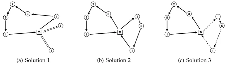
4.1 Example of different routing plans. . . 42
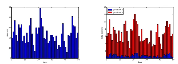
4.2 Number of requests and total demand for each day. . . 55
5.1 Number of splits and routes. . . 73
5.2 Worst Case Analysis Example. . . 77
6.1 Plot of two instances’ map. . . 119
6.2 Visual representation of the territories. . . 139
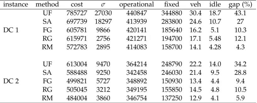
4.1 Comparison among all methods. . . 59
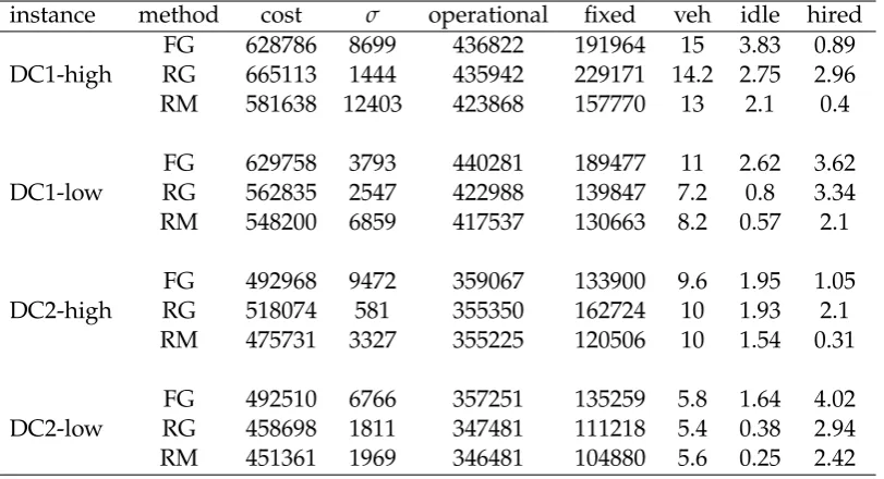
4.2 Comparison on problems with hiring option. . . 61
4.3 The effect of hiring vehicles. RM algorithm . . . 61
4.4 The effect of the route-reuse step. . . 62
4.5 The effect of the route-reuse step when including hiring.. . . 63
5.1 Routing case (bd=0) . . . 90
5.2 Fixed cost case (bd=70) . . . 91
5.3 mdanalysis - routing case . . . 92
5.4 mdanalysis - fleet size case . . . 93
5.5 Frequency analysis. . . 94
5.6 Customers’ disposition analysis. . . 95
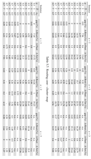
5.7 Routing case - cluster map . . . 96
5.8 Routing case - random map . . . 96
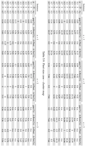
5.9 Fleet size case - cluster map . . . 97
5.10 Fleet size case - random map . . . 97
6.1 RBTA test for Duration Cost . . . 115
6.2 RBTA test for Value Cost . . . 116
6.3 Group-A instances. . . 118
6.4 Comparison between new and old approach. . . 120
6.5 Comparison with another TBR approach. . . 121
6.6 Approach validation. . . 124
6.7 Number of territories influence. . . 125
6.8 Balance cost influence. . . 126
6.9 Time Windows influence. No Balance case. . . 129
6.10 Time Windows influence. Duration Case . . . 130
6.11 Time Windows influence. TBR approach using territories designed on the noTW instances. . . 131
6.12 Demand variation influence. No Balance Case . . . 132
6.13 Demand variation influence. Duration Case . . . 133
6.14 Value variation influence. Value Case . . . 133
xx LIST OF TABLES
6.15 Frequency influence. No Balance Case. . . 135
6.16 Frequency influence. Duration Case. . . 135
6.17 Frequency influence. Value Case. . . 136
6.18 Request variation influence. No Balance Case . . . 137
6.19 Request variation influence. Duration Case . . . 137
Introduction
In this chapter, we briefly illustrate the domain to which the problems studied be-long. Moreover, we outline the objectives and contributions of this thesis. Finally, we present the structure of the following chapters.
1
.
1
Background and Motivation
One of the most active areas of Operations Research (OR) is certainly the family of Vehicle Routing Problems (VRPs). In their seminal work, Dantzig and Ramser [1959], published more than 50 years ago, Dantzig and Ramser proposed the first mathematical programming model and the first numerical method for the VRP. Since then a huge number of papers have been published, proposing new variants of the original problem, new models, exact methods and heuristic algorithms. The interest of the research community is not only motivated by the fact that the VRP constitutes a hard and challenging combinatorial problem, but also by the applicability and industrial relevance of the problem. The use of optimisation techniques in the routing industry is indeed regarded as one of the success stories of OR. It is not only due to the advent of modern computers, but also, and in particular, to the mathematical understanding of the VRPs and to the complexity and efficient implementations of all the optimisation techniques that have been proposed and studied in the literature. In the past years, the focus of the research community has partially moved away from academic extensions of the VRP and has shifted towards more realistic and in-dustrial variants. These problems deal with multi-faceted objective functions, aimed at modelling various sources of cost, uncertainty and dynamism. A variety of com-plex operational constraints are studied, aiming to better represent the needs of trans-portation providers. These problems usually go under the name of rich VRPs. There are many papers attempting to survey new trends and models in the routing liter-ature, two examples are Caceres-Cruz et al. [2015] and Lahyani et al. [2015]. An interesting paper comparing the state of the art of scientific research and commercial
xxii Introduction
software used to solve real-world VRPs is Drexl [2012a]. In this work, the author also points out the gaps that still separate the literature from real-world applications.
The VRP, as well as most of its variants, is by nature a single-period problem, i.e. it considers only one period (usually a day) of operations. However, there are areas of the literature focusing on problems featuring a longer planning horizon (multi-period). Two of the most know examples are the Inventory Routing Prob-lem (IRP, Coelho et al. [2013]; Andersson et al. [2010]; Bertazzi and Speranza [2012]) and the Periodic Vehicle Routing Problem (PVRP, Francis et al. [2008]; Irnich et al. [2014a]). These two problems offer two common examples of reasons to consider a multi-period horizon and integrate the routing component, i.e. how to deliver on each period, to the scheduling component, i.e., when to deliver. On one side, the IRP attempts to combine different phases of the supply chain, such as inventory con-trol and delivery. On the other side, the PVRP models applications where there is strong periodic component in the daily delivery operations. In both cases, integrat-ing the schedulintegrat-ing and routintegrat-ing parts of the problem can lead to substantial savintegrat-ings (Andersson et al. [2010]; Francis et al. [2008]). However, the research concerning multi-period problems is under-developed when compared to single-period VRPs. As an example, even though the IRP is probably the most studied multi-period rout-ing problem, there is no shared abstract model (Andersson et al. [2010]). Moreover, given the computational difficulty of the problem, only recently exact algorithms were introduced. Although, there are only able to solve very small instances. In fact, most methods are heuristic (Coelho et al. [2013]).
Even though there are multi-period extensions of the VRP, the vast majority of the
problems focus on optimising decisions at anoperationallevel. According to Crainic
The vast majority of papers in the routing literature are dedicated to problems at the operational level, with fewer papers studying how routing models can be exten-ded to tackle tactical problems. However, tactical decisions have a strong influence on daily operations. As an example, the object of a chapter in this thesis is the design of a fleet of vehicles. This usually requires a significant investment and is not an operation that can be done daily, but instead has to consider a long horizon. The decisions taken will affect the future operational plans over a long term. This type of problem has largely been overlooked in the literature.
1
.
2
Objectives and Contributions
This thesis focuses on tactical problems arising in routing applications. Each chapter in Part II is dedicated to a different problem. However, there are similarities in the main lines of research of each chapter that match the general objectives in this thesis. Namely, they are:
• investigate how standard routing models can be extended so that operational
decisions can be integrated into models for tactical problems;
• propose efficient solution methods for the formulated model;
• analyse the impact of the considered approaches at the operational level;
• analyse and quantify the impact of different features of models and instances
on the efficiency of such approaches.
Not all objectives are pursued in equal measure in all chapters. In the following we briefly summarise the main topics studied in each chapter of Part II, the findings and the relative publications.
xxiv Introduction
• Francesco Bertoli, Philip Kilby and Tommaso Urli. A general and scalable
column generation approach to fleet design problems. Submitted to Journal of Heuristics. 2017.
• Francesco Bertoli, Philip Kilby and Tommaso Urli. A Column
Generation-Based Approach to Fleet Design Problems Mixing Owned and Hired Vehicles.
Submitted to International Transactions in Operational Research. 2017.
The methods proposed in the chapter were object of a (pending) patent application in Australia and the United States. The references are:
• Australian Patent Application No. 2017203827
• US Patent Application No. 15/615,054
Splitting Deliveries in Routing Strategy. Chapter 5 considers the possibility of splitting deliveries in a multi-period VRP. Unlike split delivery routing as usually considered in VRP settings, we allow deliveries to be split across vehicles and across days. The main contribution is to analyse the benefits of this approach. A new prob-lem is formulated, together with a mathematical programming model and some valid inequalities to enhance it. Additionally, a simple yet effective heuristic is proposed. Finally, a theoretical and numerical analysis is presented, aimed at quantifying the savings introduced by allowing split deliveries over days, and studying the impact that different features of instances have on the possible savings. The chapter is based on the following paper:
• Francesco Bertoli, Philip Kilby and Tommaso Urli. Vehicle routing problems
with deliveries split over days. Journal on Vehicle Routing Algorithms. 2017.
Territory Design. The subject of Chapter 6 is the problem of dividing the service area for a transportation company. This falls in the category of districting prob-lems. The chapter describes the proposed approach to tackle such problems for rout-ing applications. The novelty lies in the integration of the routrout-ing decisions in the design model and solution method. This brings several advantages making it pos-sible to consider operational constraints and balance requirements that are seldom considered in the literature on territory design. Another contribution is the extens-ive computational analysis presented. This aims at studying the effectextens-iveness of the approach and quantifying the impact that different factors have on its effectiveness. The chapter is based on the following paper:
• Francesco Bertoli and Philip Kilby. Territory Design For Routing Problems.To
Other Contributions Here, we mention other contributions relative to a different research project studied during the first half of my PhD. The topics of this pro-ject were the theoretical analysis of Monte Carlo methods and their application to Stochastic Optimal Control Problems. The two main problems considered were the analysis of localisation operations in order to reduce the errors due to the system di-mension in Particle Filtering methods, and the application of Monte Carlo methods to the estimation of optimal control in stochastic systems. The following papers were produced during the time spent on this project:
• Francesco Bertoli and Adrian N. Bishop.Reducing the Bias in Blocked Particle
Filtering for High-Dimensional Systems. Available at https://arxiv.org/abs/ 1407.0220. 2014.
• Francesco Bertoli and Adrian N. Bishop. Adaptively Blocked Particle Filtering
with Spatial Smoothing in Large-Scale Dynamic Random Fields. Available at https://arxiv.org/abs/1406.0136. 2014.
• Francesco Bertoli and Adrian N. Bishop. Nonlinear Stochastic Receding
Ho-rizon Control: Stability, Robustness and Monte Carlo Methods for Control Approximation. International Journal of Control. 2017. Url: https://doi.org/10. 1080/00207179.2017.1349340
• Francesco Bertoli and Adrian N. Bishop. Monte Carlo methods for
control-ler approximation and stabilization in nonlinear stochastic optimal control.
Invited Paper at 17th IFAC Symposium on System Identification. 2015
• Francesco Bertoli and Adrian N. Bishop. An Error Analysis in the Limit
Ap-proximation in Path Integral Control. To be submitted.
1
.
3
Uncertainty in Tactical Problems
xxvi Introduction
an important and non-negligible role (Crainic [2003]). At the tactical level, uncer-tainty is still present and should not be neglected (Hoff et al. [2010]). Unceruncer-tainty is handled in different ways, depending on the problem studied. In each chapter, while we review the relevant literature, we review some of the approaches proposed in the literature that consider uncertainty. The approach we take in this thesis is to use historical data, or any other set of scenarios that is able to capture day-to-day variation in customers and demand, as the input to a deterministic model. This is similar to a scenario approach, where different realisations of the single operational days are considered. This choice is motivated by several reasons. First, it is a success-ful and powersuccess-ful approach. An example is given in Kilby and Urli [2016], where the authors show how well this approach performs on a fleet design problem. Second, but very important, it allows the design of efficient methods and algorithms. One of the reasons tactical problems have been overlooked in the literature is the high level of uncertainty (and the resulting huge size of a full stochastic model). Modelling uncertainty directly can lead to a very big and challenging problem. We attempt to use (deterministic) operational models to build models and methods for tactical problems. This allows us to leverage the efficiency and power of that the methods for operational problems have reached. One last reason is the availability of data. Many stochastic approaches make use of probability distributions in order to describe the problem. These are used directly or only for sampling purposes. If a probability distribution is not given, it must be inferred from the available data. However, we need a certain amount of data if we wish to extrapolate a reliable distribution and not always we have access to that much data. As an example, in Chapter 6, we only have a week worth of data. Attempting to fit a distribution on such a small data-set can lead to a very unreliable input in our problem, which in turn would lead to poor quality solutions. In these cases, using the available data set as input to our problem is the only viable approach. On the other hand, if we do have a probability distribu-tion available, we can use it to generate a reasonable number of scenarios as input to our problem. In each chapter, we highlight the advantages of our approach and the reasons to choose it over other approaches.
1
.
4
Thesis Outline
above. In each chapter, we present the motivation for the research carried out, a review of the relevant literature, the contributions to the field and some conclusions.
1
.
5
Notation
The problems considered in Part II are all multi-period extensions of the VRP. For the sake of clarity, we use the same notation throughout the entire thesis. Here, we introduce the main concepts, symbols and naming conventions that are recurrent in the following chapters.
• The number of customers considered is denoted by Nand the set of customers
byC={1, . . . ,N}.
• The depot is denoted by 0, and the set of all nodes in the network is denoted
byC={0, 1, . . . ,N}.
• Generally, customers are denoted using lettersior j.
• The cost of travelling between two nodesi,j2Cis denoted by cij.
• The time window of a customeri2C, is denoted by[ei,li].
• The fleet, or set of vehicles, is denoted byF= {1, . . . ,|F|}.
• The capacity of a vehiclev 2 Fis denoted byQv. In case the fleet is
homogen-eous, we only writeQ.
• The set of periods (single unit of operations, e.g., days) is denoted byD.
• Periods (i.e., days) are denoted using the letterd.
• The demand of a customeri 2 Con periodd 2 Dis denoted by qid. We write
qi for single-period problems.
• The set of routes for a routing problem is denoted withR. Super and subscripts
are used to denote dependence on other parameters, e.g.,Rdis the set of routes
Part I
Mathematical Background
Chapter2
Routing Problems
The goal of this chapter is to cover some of the background for Part II. In particular, an overview of routing problems is presented, with a particular focus on the areas relevant to this thesis.
2
.
1
The Vehicle Routing Problem
The Vehicle Routing Problem (VRP) is one of the most studied problems in the Op-erations Research community. In its simplest form the VRP is a straightforward generalisation of the Travelling Salesman Problem (TSP) and can be stated as
fol-lows. We are given a set of customersC ={1, . . . ,N}, a depot, denoted by 0, where
a fleet of identical vehicles F = {1, . . . ,|F|}is located, and the cost cij of travelling
from location i to location j for all pairs of locations in C = C[{0}. The goal is
to find a set of routes, i.e., an ordered list of customers starting and ending at the depot, so that all customers are visited by a route and the total distance travelled is minimised. Arguably, the most known version of the VRP is the Capacitated VRP
(CVRP). In this version, each customeri 2 Chas a demand qi 0, representing the
amount of goods to be delivered, and all trucks have a limited capacity Q > 0. A
route is feasible only if the sum of the loads of customers visited by a route does not exceed the capacity. Here and in all the following chapters, we assume that the
triangular inequality for the costscij is valid.
The VRP was originally introduced in Dantzig and Ramser [1959], where a first mathematical programming formulation and solution method were presented. The
VRP is known to be aN P-hard problem (Karp [1972]).
In next sections, we briefly present some of the most common extensions and variants of the classic VRP. The presentation is by no means exhaustive. For a more comprehensive survey we refer to the paper by Laporte (Laporte [2009]) and the book by Toth and Vigo (Toth and Vigo [2014]).
2
.
2
Routing Problems
The classification of routing problems is a task hard enough to have several survey papers and books dedicated to it. In this section, we present some extensions and characteristics of particular interest in this thesis. There are many features and exten-sions hereby not considered, such as stochastic and dynamic extension, for which we refer to the surveys in Laporte [2009]; Caceres-Cruz et al. [2015]; Hasle and Kloster [2007] and the book Toth and Vigo [2014].
2.2.1 Requests
In the CVRP the requests are described as demands for goods that have to be satisfied by a route. Here we look at some requests’ features that arise in different routing problems.
Time Windows. Amongst the most studied and practically relevant constraints as-sociated with requests are those related to time. In the VRP with Time Windows (VRPTW, Cordeau and Groupe d’études et de recherche en analyse des décisions
[Montréal(2000]) the time tij needed to travel between pairs of locations i,j 2 C, a
time window[ei,li]and a service timesi for each customeri2Care considered.
Cus-tomers can only be visited during their time windows. Usually, vehicles are allowed to arrive early and wait at a location before the start of a time window. The service time represents the time needed to complete service at the customer’s location. In some problems, multiple time windows for each customer are considered (Pesant et al. [1999]; Vidal et al. [2014]).
Time windows are not always imposed ashardconstraints. In Taillard et al. [1997],
the authors introduce the VRP with Soft Time Windows (VRPSTW) where early and late arrivals are allowed but penalised by using a convex function. The most common penalty functions used to penalise time windows violations are piece-wise linear functions. A mix of penalty functions and/or bounds on late service or early arrivals is also possible.
§2.2 Routing Problems 5
to another one (delivery). If no transhipments are allowed, then the same vehicle must visit both locations and the pickup must be performed before the delivery.
Split Deliveries. In the CVRP, requests can only be performed by a single vehicle. However, there are many reasons to consider the possibility of splitting the service of a customer across multiple vehicles. One simple example is if some demands exceed the capacity of the biggest truck. In Dror and Trudeau [1989], the authors introduce the Split Delivery VRP (SDVRP). This is a straightforward extension of the CVRP where it is no longer assumed that a request has to be satisfied by a single vehicle. Allowing a delivery to be split adds a considerable complexity to the problem but can also lead to considerable savings, up to 50% (Archetti et al. [2006a]).
Profitable Routes. It is not possible to satisfy all requests in all applications, due to capacity and time limitations. In order to select the requests to be fulfilled, one can penalise the unassigned requests or reward the ones that are included. The literature on routing problems with profits is vast. The academic formulations go from simple extensions of the TSP (Tsiligirides [1984]) to extensions of the VRP (Butt and Cavalier [1994]). A survey can be found in Archetti et al. [2014b].
Multi-Commodity Routing. One somewhat overlooked class of problems are those where customers’ demands are made of several commodities. Some authors have proposed academic extensions of the VRP (Archetti et al. [2014a, 2015a]) to include more than one commodity. Multi-commodity routing applications are common in practice: two examples, which are the problems that motivated the work presented in Chapter 4, are: the delivery of fuel to gas stations and the delivery of grocery to supermarkets. In the former, the different types of fuel, that may not be mixed, are the commodities. In the latter, one has to differentiate between products that need, or do not need, to be transported in a refrigerated truck.
2.2.2 Routes
operatewithina route. A more comprehensive list of route constraints and structures can be found in Irnich et al. [2014b]; Drexl [2012a].
Resources. Simple constraints can be imposed on a route’s length and time. These could be due to working regulations or a need to limit the consumption of some resources (see Laporte et al. [1984] for an example). Obviously, capacity can be con-sidered as another limited resource.
Depot Visits. Another assumption in the CVRP is that a vehicle cannot return to the depot while performing a route. However, this assumption is often not true in practice, as vehicles are allowed to visit the depot to refill or unload. In Taillard et al. [1996], the authors introduce the VRP with Multiple use of vehicles to model and study this situation. This problem is also known as the Multi-Trip VRP (Cattaruzza et al. [2014]; Battarra et al. [2009]). An example of a real-world problem allowing for multiple trips is the problem studied in Chapter 4.
Balanced Routes. One example of an inter-route constraint, which has not received much attention, is the balance of the routes with a particular measure (Drexl [2012a]; Jozefowiez et al. [2008]). For example, a company may wish to have daily routing plans that are fair to the drivers in terms of time (Jozefowiez et al. [2007]). If a driver is paid proportionally to the load carried (Lee and Ueng [1999]), or the number of requests served (as in technicians routing) a fair division of the demand between the routes is essential. This matter is explored in more detail in Chapter 6.
Geometric Properties of Routes. In the majority of routing problems, the geomet-ric properties of the routes are ignored. However, these may be of practical relev-ance in real-world applications. Some papers (Lu and Dessouky [2006]; Constantino et al. [2015]) have proposed different measure to make routes visually appealing.
One other important concept is that of regionalization, as defined in Mourgaya and
Vanderbeck [2007], of the routes. This is related with the goal of having drivers that are familiar with their service area. More references are given in Chapter 6.
2.2.3 Fleet
§2.2 Routing Problems 7
Heterogeneous Fleet. In the CVRP the vehicles are assumed to be identical. How-ever, this is rarely the case in reality, as fleets are usually composed of different types of vehicles. The difference in the available vehicles might be reflected, for example, in different capacities and different travelling times and costs. Moreover, the fleet is not always given as an input; instead its composition can be a decision variable. If so, the cost of purchasing a vehicle can differ based on its type. A classification of the problems considering a heterogeneous fleet is given in Baldacci et al. [2008]. A more industrial oriented survey can be found in Hoff et al. [2010]. In Chapter 4, a more detailed survey on this topic is presented.
Compatibilities. Heterogeneous fleets give rise to compatibility constraints. Com-mon reasons for incompatibility are access limitations, due to size or regulations, to a customer’s location. These compatibilities may also be due to drivers’ qualifications.
Multi-Compartment Vehicles. The counterpart of multi-commodity requests are multi-compartment vehicles. The number of compartments can be fixed, and each compartment can be dedicated to a single commodity (Mirzaei and Wøhlk [2017]) or several (Urli and Kilby [2017]). If the compartments take the form of trailers, there can be a variable number of trailers for each truck. This is the problem modelled by Chao in the Truck and Trailer Routing Problem (Chao [2002]). In Drexl [2013], the trailers can be exchanged between trucks during a route.
Multi-Depot. The vehicles might start and end at different depots. If the fleet is homogeneous, the problems is known as Multi Depot VRP (Renaud et al. [1996b]). Variation of this problems consider only the starting point of a vehicle while the end location is left open (Vidal et al. [2014]).
External Resources. Whenever the available fleet is not sufficient to meet all re-quests, a company might resort to hiring extra vehicles. The problem of sub-contracting some of the requests to external transportation providers appears in the literature in different areas. In Kopfer and Wang [2009] the authors discuss this problem, present-ing different business options.
2.2.4 Objectives
used. If an objective is multi-dimensional, a hierarchical structure may be imposed. As an example, in the set of benchmark problems for the VRPTW presented in So-lomon [1987], the first objective is to minimise the number of vehicles while the second is to minimise the total distance. If no hierarchy is assumed, the objective is a weighted sum of one dimensional objectives. Another source of cost are the
con-straints that are modelled as soft constraints. For example, a violation of the time
windows may be allowed, but penalised, as discussed in (Taillard et al. [1997]). The survey presented in Jozefowiez et al. [2008] focuses on multi-objective optimisation in routing problems.
2
.
3
Multi-Period Problems
All of the VRP extensions presented in the previous section are of a single-period nature, i.e., the horizon considered is made up of only one period of operation. A part of the literature is dedicated to multi-period problems. Since periods are usu-ally days, we use these two terms interchangeably in what follows. The reasons to introduce a multi-period horizon are several and of different nature. In some trans-portation systems, a single day might be not enough to describe the problem due to long distances (Savelsbergh and Song [2007]). One other reason is to integrate other aspects in the problem formulation. Two examples are provided by the well-known classes of problems denoted by Periodic VRPs (PVRPs) and Inventory Routing Prob-lems (IRPs). In the former, the goal is to model a periodicity of the problem and integrate delivery-pattern schedule and routing. In the latter, the goal is to integrate inventory control and routing. Considering more than one period adds considerable complexity to the problems, but, on the other hand, offers the possibility for higher efficiency and cost savings. In this section, we consider some multi-period extensions of the VRP.
§2.3 Multi-Period Problems 9
maintenance services (Hadjiconstantinou and Baldacci [1998]) and health care (Hem-melmayr et al. [2009]).
Inventory Routing Problems. In IRPs, there are no requests placed by customers. Instead, a vendor must decide when to visit each customer, how much to deliver and a routing plan for every day in the horizon (a business model called Vendor Managed Inventory). Usually a “consumption rate” for each customer is available and stock-outs are forbidden. The idea behind IRPs is to have a centralised control for both inventory and routing, integrating two parts of the supply chain that are usually controlled separately. This approach has specific applicability in real-world problems, as it requires complete control over the customers’ inventory level, and also some form of knowledge of the rates of consumption. However, if such a deep integration of the inventory management and routing aspects is feasible, the possible savings are substantial (Andersson et al. [2010]). We refer to Coelho et al. [2013]; Bertazzi and Speranza [2012] for academic oriented survey on IRPs. An industrial point of view presented in Andersson et al. [2010].
Service Consistency. Another reason to consider a multi-period horizon is to in-crease the level of consistency in service. In Groër et al. [2009], the authors introduce the Consistent VRP (ConVRP) which is a multi-period routing extension of the VRP where the goal is to design daily routing plans so that customers are always visited by the same driver at approximately the same time. This problem was later extended in Kovacs et al. [2014] to have an assignment of teams of drivers to customers. Other examples of papers using multi-period routing models to improve service consist-ency are Smilowitz et al. [2013]; Schneider et al. [2014]; Wong and Beasley [1984]. The matter of improving consistency is analysed more in depth in Chapter 6.
2
.
4
Tactical Routing Problems
As mentioned in the Introduction, according to Crainic [2003], transportation
sys-tems management can be divided in three levels: strategical, tactical and operational.
These three levels differ in the length of the horizon considered, from the longest (strategic level) to the shortest (operational level), and, consequently, also in the type of decisions taken, and the uncertainty faced. Examples of the decisions involved are: demand modelling and location of facilities for the strategic level, service net-work design and resource acquisition for the tactical level, routing and loading of vehicles for the operational level. In Crainic [2003], it is noted that decisions taken at a particular level influence lower levels and provide useful information to higher levels.
Tactical problems do not (only) focus on routing decisions, as these will likely be re-optimised and changed in the future, but also on issues that can be placed one step above in a decisional hierarchy. Some examples of tactical problems are considered and analysed in this thesis: the design of a fleet for a medium to long term or the districting of a service area for routing services such as grocery delivery or winter gritting operations. The literature on these topics is reviewed in the chapters of Part II. One other important example of tactical problems is the Location-Routing Problem (LRP, Nagy and Salhi [2007]. While facility location problems are more of a strategical nature (Crainic [2003]), the LRP can be described as follows: given a set of potential depots, costs for opening such depots, a homogeneous fleet and a set of customers with known demands, identify a subset of depots to be opened, assign customers to them, and determine vehicle routes so to minimise the total cost. A survey on LRPs is Prodhon and Prins [2014].
Both IRPs and PVRPs lie somewhere in the middle between tactical and opera-tional levels. Most papers study these problems at an operaopera-tional level. However, there are examples of real-world applications (Gaur and Fisher [2004]) that consider a medium to long time horizon. The integration of production and routing decisions is a topic of increasing interest. A survey of optimisation models dedicated to the study on this integration can be found in (Díaz-Madroñero et al. [2015]).
Chapter3
Solution Methods
In this chapter an overview of the methods used to solve VRPs is given, with a particular focus on the techniques that are used in Part II. The first two sections are dedicated to exact methods, and, in particular, to column generation. The last sections present an overview of heuristic methods, focusing in particular on local and meta-heuristic search.
3
.
1
Exact Methods
The research on exact methods for VRPs has been developed for over 40 years. The work done in this area is quite detailed and a survey is out of the scope of this section. Here, we briefly present the topic and refer to Semet et al. [2014] for a detailed overview on early methods, and to Poggi and Uchoa [2014] for an overview on new methods using set partitioning formulations.
The basic formulation for CVRP makes uses of binary flow variables xij to
rep-resent whether a vehicle travels on the arc connecting node i to node j for all i,j 2
C(= C[{0}). The problem can be formulated as follows:
min
Â
i,j2C
cijxij (3.1)
s.t.
Â
j2C
xij =1 8i2 C (3.2)
Â
j2Cxji=1 8i2 C (3.3)
Â
j2Cx0j =|F| (3.4)
Â
i2S,j2/Sxij r(S) 8S✓C,S6=∆ (3.5)
xij 2{0, 1} 8i,j2 C (3.6)
The objective (3.1) minimises the total travelling costs. Note that, ifcij =cjifor all
i,j2C, the CVRP is said to be symmetrical, otherwise it is said to be asymmetrical.
Constraints (3.2) and (3.3) impose that each customer must be visited and must have exactly one predecessor and one successor. Constraint (3.4) sets the number of routes
equals to the fleet size (note that a route can be empty). In constraints (3.5), r(S)
represents the minimum number of routes needed to satisfy the total demand of the
subsetS. In the CVRP, this can be computed through a bin packing problem. Usually,
instead of r(S), the lower bound dÂi2Sqi/Qeis used. Integrality of the solution is
imposed by constraints (3.6). Note that constraints (3.5) serve at the same time as
capacity and subtour elimination constraints. To see the former, consider S, the
set of customers in a router. The associated constraint (3.5) can be transformed into
Âi2Sqi Q. A similar argument can be made for the subtour elimination constraints.
This model was originally introduced in Laporte et al. [1986].
It is well known that the number of constraints (3.5) grows exponentially withN.
Therefore, it is not practical, if at all possible, to include all of them in the formulation. One possibility is to solve the problem without such constraints, check if the solution
violates some of them (a process named separation), in which case these are added
to the formulation and the process is restarted. This procedure gives rise to cutting-plane algorithms. One other possibility is to include additional variables to represent the load (or the time, especially if one considers time windows) of a vehicle arriving
at a customer’s location. For example, if for each node i 2 C we denote by ui the
load of the vehicle upon arrival ati, one would add the following constraints:
§3.1 Exact Methods 13
to replace the subtour elimination constraints, and
qi ui Q 8i2C
to replace the capacity constraints. The resulting model is known asMTZ-formulation.
as it was originally proposed by Miller, Tucker and Zemlin in Miller et al. [1960]. This
type of model is called two-index (vehicle) flow formulation. In some extensions of
the CVRP, one may need to make the vehicles explicit in the flow variables, using
therefore athree-indexflow formulation.
This type of model is solved using branch-and-bound or branch-and-cut tech-niques, or mixtures of the two. A lot of effort has been spent on studying branching and lower bounding techniques to enhance the performance of the solution meth-ods. Also, many different families of valid cuts have been introduced to strengthen the mathematical programming models for the CVRP, and many methods have been proposed for cut separation, i.e., to quickly identify violated cuts. An overview of this work can be found in Semet et al. [2014].
3.1.1 Set Partitioning Formulations
The Set Partitioning (SP), or Set Covering (SC), formulation for the CVRP was first
introduced in Balinski and Quandt [1964]. Consider the setRof all possible routes for
a CVRP instance. A binary variable xr is associated to each router 2 Rto represent
whether or not we user. Moreover, the cost of routeris denoted bycr, and, for each
customer i 2 C, the binary parameter ari denotes whether r visitsi. The SP model
follows:
min
Â
r2R
crxr (3.7)
s.t.
Â
r2R
arixr =1 8i2 C (3.8)
Â
r2Rxr =|F| (3.9)
xr2 {0, 1} 8r2 R (3.10)
Constraints (3.8) impose that each customer is visited by exactly one route. Con-straint (3.9) requires the number of selected routes to equal the fleet size. It is possible
to replace the sign of this constraint toor to add|F|copies of the empty route toR
to allow for idle vehicles. Integrality of the variables is imposed by constraints (3.10).
Since a solution of this model is, in particular, a partition of C, this formulation is
one obtains a Set Covering formulation. Note that from a solution of SC we can obtain a solution of SP by, possibly, dropping customers from routes. Moreover, if the triangular inequality for travelling costs is satisfied, dropping customers cannot result in an increase of the cost. Therefore, there exists an optimal solution of SC that is also an (optimal) solution for SP. The main reasons to use SC instead of SP are that, in the former, amongst routes with the same costs, only inclusion-maximal feasible circuits need to be considered. Moreover, as the dual variables associated with constraints (3.8) have to be non-negative in the SC dual problem, the dual space is considerably reduced.
The issue with SP or SC formulations lies in the huge number of variables. The enumeration of all possible routes is out of reach for reasonable sized problems. Consequently, it is not possible to solve the model directly. Instead, one has to resort to Column Generation (CG). Since CG is the topic of next section we postpone a few remarks on the use of CG in the routing literature. To conclude this section, we only mention that, since the seminal work of Desrosiers, Soumis and Desrochers (Desrosiers et al. [1984]), the SC formulation, in combination with CG, has been the dominant approach for exact methods for the VRPTW. According to Poggi and Uchoa [2014], this type of method can consistently solve instances of 200 customers. In Pecin et al. [2017], two instances of 200 customers each are solved with computational times of about 1, and 11 hours. Research to improve exact methods for CVRP and VRPTW is still ongoing (Uchoa et al. [2017]).
3
.
2
Column Generation
In this section, the main goal is to describe Column Generation and its relation to Dantzig-Wolfe decomposition. At the end of the section, we briefly overview the use of CG in the VRP literature.
Column Generation is a useful technique when a mathematical problem cannot be directly solved due to its high number of variables. Consider the following linear problem:
[P] minc>x (3.11)
s.t. Ax=a (3.12)
x 0 (3.13)
where x2Rn,a 2Rm and A2Rm⇥n. At each iteration of the simplex method, only
§3.2 Column Generation 15
generation, is to avoid generating and considering these columns. We denote by Aj
a column of problemP, and by cj its cost coefficient. We define J = {1, . . . ,n}, the
index set of all columns. The master problemis the following linear program, which
is a reformulation of problemP:
(MP) min
Â
j2J
cjxj (3.14)
s.t.
Â
j2J
Ajxj =a (3.15)
xj 0 8j2 J (3.16)
In the simplex method, at each iteration, one looks for a non-basic variablej2 J with
negative reduced cost to enter the basis. If no such column is found, the current basic solution is optimal. CG mimics the simplex method, with the only difference being
that, in CG, at each iteration, only a (small) subset J of J is available. The master
problem, reformulated using only the subset J is calledrestricted master problem, and
is denoted by RMP in what follows. We assume that the set J contains a feasible
solution for RMP. If this cannot be guaranteed, then RMP has to be moified to
ensure feasibility. At each CG iteration, RMP is solved, and the dual variables p,
associated with constraints (3.15), are computed. Then, the goal is to identify a new
column with negative reduced cost (note this cannot be in J by linear programming
theory (Bertsimas and Tsitsiklis [1997])). In order to do this, one solves the following
minimisation problem, called thesub-problem:
c⇤(p) =min{cj p>Aj | j2 J} (3.17)
The objective in the sub-problem is precisely the current reduced cost of a column. Because the dual variables are sometimes called shadow prices, the sub-problem is
also referred to as the pricing-problem. If the optimal value of the sub-problem is
non-negative, the optimal solution ofRMP is also optimal forMP and therefore for
P. Otherwise, the minimising column is inserted in J and the process starts again.
The CG algorithm has to be initialised with a starting set of columns. Usually, these are obtained using a heuristic method to “warm start” the solution. Algorithm 1 summarises the CG method.
We denote with z⇤ andz⇤
RMP the optimal values ofMP andRMP. At each
itera-tion, the current valuezRMPofRMP is an upper bound for both quantities. Moreover,
given that the cost of a linear problem cannot be reduced by more thanÂj2Jxj times
Algorithm 1Column Generation
1: Fix a starting subset J ✓ J of columns
2: SolveRMPusing the columns in J
3: Obtain the associated dual variablesp
4: Solve the sub-problem usingp
5: ifc⇤(p)<0then
6: Identify the columnjthat is the minimiser of the sub-problem
7: Addjto J and go back to Step 2
8: else
9: Stop. The current solution is optimal forMP.
10: end if
derived.
zRMP+c⇤(p)
Â
j2Jxj zMP⇤ z⇤RMPzRMP (3.18)
The lower bound can be used to compute an optimality gap. Note that, ifc⇤(p) =0,
thenz⇤
MP= zRMPand optimality follows.
It is clear that a key part in the CG algorithm is Step 4. Indeed, one has to find an efficient way to generate new columns. Usually, the sub-problem has a special structure to make it possible to efficiently solve it without enumerating all columns. A relevant example, coming from the application of CG to VRPs, is provided later in Section 3.2.4.
3.2.1 Common Issues
There are many potential issues and delicate questions in the implementation of CG. In the following, we mention some of the issues that typically arise. We refer to Lübbecke and Desrosiers [2005] for a more detailed presentation.
Managing Columns. First of all, one has to decided how to manage the set J. The number of generated columns can become very high and consequently slows down
the solution ofMP. Options range between keeping all generated columns and only
the ones in the current optimal basis (Lübbecke and Desrosiers [2005]; Bertsimas and Tsitsiklis [1997]).
§3.2 Column Generation 17
solve the dual problem of MP. This also helps to overcome potential numerical
is-sues in the computation of the dual variables and facilitates numerical stabilisation techniques, which are presented later in the section. Degeneracy is also a problem to be considered. A typical issue is that newly generated columns do not decrease the objective as the current solution is degenerate. This can slow down the process considerably.
Sub-Problem Another matter is the number of columns to be generated at each iteration and how they are generated. The generation of a column usually involves solving an integer problem. Several solution techniques, such as dynamic program-ming, might produce several columns with negative reduced cost. Therefore, one
has to choose whether to insert all of them in J, or choose only the one with smallest
reduced cost. Moreover, the sub-problem does not have to be solved to optimality at each iteration, since we only need one column with negative reduced cost.
It is very common, to speed up the solution of the sub-problem, to use heuristic, especially in the first iterations. When these heuristics fail to obtain a column with negative reduced cost, the sub-problem is solved to optimality. Note that this is also
needed to check the optimality of the currentMP solution. The efficient solution of
the sub-problem is arguably the most important step in CG. In Vanderbeck [1994],
a concept of dominance for columns is introduced. This is meant to help excluding
columns that cannot ever be optimal in the sub-problem because there will always be another column with lower reduced cost. All of these issues are discussed in more detail in Lübbecke and Desrosiers [2005].
Tailing-off Effect. Another important issue is the tailing-off effect. In the last itera-tions, the columns found have negative reduced costs close to zero, causing small or possibly null improvements in the objective. This is also due to the poor convergence properties of the simplex method. Other solution methods for the master-problem can help closing the optimality gap faster. The matter is discussed in more detail in Lübbecke and Desrosiers [2005]. Moreover, if CG is embedded in a branch-and-bound algorithm, lower branch-and-bounds are used to prematurely stop the execution of a node. Typical lower bounds are lagrangian-type bounds that are based on equation (3.18).
3.2.2 Dantzig-Wolfe Decomposition
We now focus on the relation between CG and the Dantzig-Wolfe decomposition (Dantzig and Wolfe [1960]). Consider the following linear problem:
(O) mind>x
s.t. Bx= b
Dx=d x 0
(3.19)
which we refer to as the original formulation. To keep the presentation concise, we
assume that the solution space of problem O is bounded. This assumption is not
necessary and easily removed (see Lübbecke and Desrosiers [2005]; Bertsimas and Tsitsiklis [1997]). Nonetheless, it is satisfied by the problems considered in Part II.
We define the following set, X = {x 2 Rn|Dx = d,x 0} 6= ∆ and let {xj}j2E be
the set of extreme points ofX. It is well known that any x2Xcan be represented as
a convex combination of its extreme points. That is,
x=
Â
j2E
ljxj where
Â
j2E
lj =1 and lj 0, 8j2 E
We set cj = c>xj and Bj = B xj. By using the above equation, problem O can be
§3.2 Column Generation 19
(DW-O) min
Â
j2E cjlj
s.t.
Â
j2E
Bjlj =b (3.20)
Â
j2Elj =1 (3.21)
lj 0 8j2E
This plays the role of the master problem in the previous section. Note that
only the constraints associated with matrix B are part of the new formulation. The
ones associated with D are now included in the definition of the variables. Since
the size of X is usually huge, one resorts to using CG. The columns of this new
formulation are the extreme points {xj}j2E. Therefore, it is essential for the set X
to have a special structure. We denote by athe vector of dual variables associated
with constraints (3.20) and with q the dual variable associated with constraint (3.21)
(which is called theconvexity constraint). The sub-problem can be written as:
min{cj a>Bj q | j2 E}
Now that the master and sub-problem are defined, CG can be applied. Note that, thanks to the convexity constraint, the lower bound (3.18) now takes the form
zRMP+c⇤(p)zMP⇤ zRMP.
In the literature, the constraints defined by the matrix Bare called the
complicat-ing constraints, and define the master problem. On the other side, the ones defined
by the matrix D are used to define the structure of the sub-problem.
Mathematic-ally speaking, the Dantzig-Wolfe decomposition can be described as follows: given a linear problem, one splits the set of constraints in two parts, a set of complicating constraints and a set of constraints that are used to define a new search space. This
latter set defines a polygon P in the original search space. Note that every point in
the original search space is contained in P. Since every point in Pcan be expressed
process to have some benefits,Pmust have a special structure that one can exploit to efficiently find extreme points.
In many applications, the matrix Dhas a diagonal structure
D= 0 B B B B @
D1 D2
...
Dk
1 C C C C
A, d= 0 B B B B @
d1 d2
...
dk
1 C C C C A
where each blockDi 2Rm⇥ni andÂki=1ni =n. If one defines
Xi ={x2Rni|Dix =di,x 0}, i=1, . . . ,k
the Dantzig-Wolfe decomposition can still be used, except that now we have k sets.
Geometrically, polygon Pis decomposed1 intok polygons, each one associated with
matrixDi, and with its own extreme points. Therefore, we can split the sub-problem
into k separated sub-problems. The CG algorithm does not change. At each
iter-ation, we solve k sub-problems to identify new columns. Note that not all of the
sub-problems have to be solved at each iteration, as only one column with negative reduced cost is needed. However, all of them has to be solved to optimality to prove
the master problem optimality (Step 9). Finally, ifc⇤
i(p)denotes the value of thei-th
sub-problem, the lower bound (3.18) can be rewritten as:
zRMP+ k
Â
i=1c⇤
i(p)z⇤MPzRMP.
3.2.3 Integer Problems
Because one needs the dual variables to solve the sub-problem, the master problem
(and thus the original problemP) has to be linear. If the original problemOis integer,
one has to add the integrality constraint
Â
j2Eljxj 2 Zn
to the problemDW-O. In this case, CG has to be embedded in a branch-and-bound
scheme, obtaining what is called abranch-and-price (BAP) method. If valid cuts are
progressively added to the formulation, sometimes the method is called
branch-and-cut-and-price. One interesting remark is on the branching strategy. This must not
§3.2 Column Generation 21
rupt the structure in the sub-problem, causing any difficulty in efficiently solving the sub-problem. An example, clarifying this concept, is presented later in Section 3.2.4.
3.2.4 Column Generation Applications in Routing Problems
When applied to VRPs, CG, in combination with the SP (or SC) formulation has proved very successful. The idea was first applied to VRPTW in Desrosiers et al. [1984]. The SP formulation (3.7-3.10) can be obtained by applying the Dantzig-Wolfe decomposition to the flow formulation (3.1-3.6), by moving the subtour elimination constraints (3.5) into the sub-problems, and by dividing constraints (3.3) and (3.2)) between master and sub-problem. In the master problem, one keeps the requirement to visit all customers, while in the sub-problem one imposes flow conservation
con-straints. The polygon P, defining the sub-problem search space, is made up by all
feasible routes. The sub-problem takes the form of a (Elementary) Shortest Path Prob-lem with Resourced Constraints (SPPRC, Irnich and Desaulniers [2005]). SPPRCs are usually solved by means of a forward dynamic programming labelling algorithm (Ahuja et al. [1993]). In a nutshell, the idea is to create partial paths starting from the depot and progressively extend them to other nodes. Paths are eliminated based on dominance rules. A dominance rule’s job is to make sure one does not keep memory of sub-optimal paths. More details can be found in Irnich and Desaulniers [2005]; Ahuja et al. [1993].
As mentioned before, since VRPs are integer problems, some care must be taken when defining a branching strategy for BAP methods. For example, fixing a variable
xr=0 in the master problem destroys the sub-problem structure, or, to be more
the algorithm. Some authors eliminate only 2-cycles (Christofides et al. [1981]), which has been shown to improve performance. Other authors have introduced a relaxed concept of “route”. For example, in Christofides et al. [1981]; Fukasawa et al. [2006],
the authors introduce the concept of q-route; that is, a route that is allowed to visit
a customer twice, but only if at least another k customers are visited between the
repeated visits. In a post processing phase, q-routes can be easily transformed in
elementary routes. For a more detailed presentation we refer to Poggi and Uchoa [2014].
In the literature concerning routing problems, several heuristic methods are based on CG (Mourgaya and Vanderbeck [2007]; Ceselli et al. [2009]; Bertoli et al. [2017b,c]; Taillard [1999]). A classification of CG-based heuristics can be found in Joncour et al. [2010]. In Rousseau et al. [2004], the authors propose using Constraint Programming (Rossi et al. [2006]) to solve the pricing problems.
Finally, it is worth mentioning that CG-based algorithms have successfully been applied into a variety of routing problems such as: fleet size and mix problems (Choi and Tcha [2007]; Baldacci and Mingozzi [2009]), SDVRPs (Archetti et al. [2015a]), dynamic routing (Chen and Xu [2006]), PVRPS (Mourgaya and Vanderbeck [2007]), IRPs (Le et al. [2013]; Oppen et al. [2010]) and rich VRPs (Ceselli et al. [2009]). Many papers do not attempt at solving a problem exactly but only propose heuristics based on the CG algorithm.
3
.
3
Heuristic Methods
§3.3 Heuristic Methods 23
3.3.1 Constructive Heuristic
Constructive heuristics are mostly used to provide a starting solution for improve-ment heuristics. One of first methods proposed was the Clarke and Wright’s Saving heuristic (Clarke and Wright [1964]). The idea is very simple: one first builds a
route of the form (0,i, 0) for each customeri2C. Successively, the algorithm merges
pairs of routes. To be precise, merging a route (0, . . . ,i, 0) to (0,j, . . . , 0) results in the
route (0, . . . ,i,j, . . . , 0), i.e., routes are connected end to start. The pair to be merged
is chosen, among all pairs that would yield a feasible route, based on the savings obtained by merging the two routes.
Other constructive method are based on the route-first cluster-second algorithm,
originally proposed in Beasley [1983]. The idea is to first solve a TSP for all custom-ers and then split the so obtained giant-tour in smaller routes. However, this type of
method is seldom used. A contrasting principle is the cluster-first route-second
prin-ciple. Algorithms of this type attempt to first create clusters of customers and then solve a TSP for each cluster. Two well-known examples are the Fisher and Jaiku-mar method (Fisher and JaikuJaiku-mar [1981]) and the sweep heuristic (Gillett and Miller [1974]). In the former, a partition of the customers is obtained by solving an as-signment problem with an objective function approximating the routing cost. In the latter, clusters are formed based on the polar coordinates of the customers’ location.
Insertion heuristics constitute another type of constructive methods. The typical insertion heuristic is structured as follows: first it chooses a seed customer, usually the one farthest from the depot, or the most urgent one (if time windows are con-sidered), to initialise a route. Successively, customers are chosen and inserted in the route, one at the time. If no more feasible insertion is found, the algorithm “opens” a new route by choosing a new, still unrouted, seed customer and the insertion process starts again. Candidate insertions are evaluated with metrics combining geographical and other information, e.g., time-related. One of the most successful insertion heur-istics for the VRPTW is the I1 method, originally proposed by Solomon (Solomon [1987]). The method evaluates the best insertion of each customer using a metric accounting for distance saving and time delay due to the insertion. Successively, the insertion to be performed is chosen using a different metric, that rewards customers far from the depot. For a more detailed presentation of the I1 heuristic and related modifications, we refer to Bräysy and Gendreau [2005a]. These types of insertion
heuristic are calledsequential, as they build one route at the time. Conversely, there
3.3.2 Improvement Heuristics
Improvement heuristics attempts to improve a given solution by modifying its struc-ture. Based on an initial solution to start the improvement process. Classical methods perform intra-route and inter-routes moves. Most of the intra-route moves were
ori-ginally designed for the TSP. Examples are the 2-opt and l-opt moves (Bräysy and
Gendreau [2005a]; Toth and Vigo [2014]). Examples of inter-routes moves are the
relocatemove, where a customer is removed from its original position and relocated
somewhere else; the swapmove, where two customers are swapped; or the 2 opt⇤
move, that is an extension of the 2-opt move involving two different routes (Toth and Vigo [2014]). Since all of these moves are formally defined, it is possible to ex-haustively enumerate all the solutions that can be obtained applying one particular move. Such exploration can be computationally expensive. However, a smart im-plementation of the exploration can considerably reduce the number of possibilities to be evaluated. For example, in Savelsbergh [1992], the authors illustrate how to speed-up the search of the neighbourhood defined by a 2-opt for a TSP solution.
Other types of method are not defined by specific moves but attempt to improve a solution by alternating methods that partially destroy a solution (i.e., they remove customers from it), and then repair the solution. A well-known example is the Large Neighbourhood Search heuristic (Shaw [1998]), which we present in detail later in this chapter.