On the complexity of hybrid logics with binders
Balder ten Cate
∗Massimo Franceschet
†Draft February 1, 2005
Abstract
Hybrid logicrefers to a group of logics lying between modal and first-order logic in which one can refer to individual states of the Kripke struc-ture. In particular, the hybrid logic HL(@,↓) is an appealing extension of modal logic that allows one to refer to a state by means of nominals and to dynamically create names for states.
Unfortunately, as for the richer first-order logic, satisfiability for
HL(@,↓) is undecidable and model checking for HL(@,↓) is PSpace -complete. We carefully analyze these negative results and establish re-strictions (both syntactic and semantic) that make the logic decidable again and that lower the complexity of the model checking problem.
1
Introduction
There is a general interest in well-behaved logical languages in-between the basic modal language and full first-order logic. Ideally, one would like such languages to combine the good properties of both: to be reasonably expressive, to be decidable, and to have other good properties, such as the interpolation property.1
Famous examples of fragments that have been studied are theguarded frag-ment [1, 15] and the two variable fragment [20, 16]. Both are decidable, rea-sonably expressive languages, but they lack interpolation. The hybrid logic
HL(@,↓) is another example of a language in between the basic modal lan-guage and full first-order logic. It extends the basic modal lanlan-guage with three constructs: nominals, which act as names of states of the model, satisfaction operators, which allow one to express that a formula holds at the state named by a nominal, and↓, which allows one to give a name the current world. To-gether, these three elements greatly increase the expressivity of the language.
∗Informatics Institute, University of Amsterdam, The Netherlands. Email: [email protected]
†Informatics Institute, University of Amsterdam, The Netherlands; Department of
Sci-ences, University of Chieti and Pescara, Italy. Email: [email protected]
1Interpolation is an important property of logics. Logics that have interpolation are in
Moreover, like the basic modal language and full first-order logic,HL(@,↓) has the interpolation property. Unfortunately, it is undecidable.
In this paper, we given an in-depth analysis of the undecidability of
HL(@,↓). We show how decidability can be regained by making a syntactic restriction on the formulas, or by restricting the class of models in a natural way. Moreover, we show how these and similar syntactic and semantic restric-tions affect the complexity of the model checking problem for hybrid languages. Incidentally, it should be emphasized that HL(@,↓) is a proper fragment of first-order logic, and in fact a very natural fragment. It is the generated submodel invariant fragment of first-order logic [4], it is the least expressive extension of the basic hybrid language HL(@) with interpolation [10], and, finally, it can be characterized as the intersection of first-order logic with second order propositional modal logic [9]. Some of the results reported in this paper can be seen as evidence thatHL(@,↓) is better behaved than first-order logic. The paper is as follows. In Section 2 we introduce hybrid logic and we show that it is a fragment of first-order logic, while in Section 3 we revisit the undecidability result forHL(@,↓). We show how decidability can be regained by restricting the language in Section 4 and by restricting the class of models in Section 5. In Section 6 we investigate how these and similar restrictions affect the complexity of the model checking problem for hybrid logic, and we conclude in Section 7.
2
Hybrid Logic
In this section we introduce hybrid logic and we show that it is a fragment of first-order logic. We assume the reader familiar with modal logic [6].
In its basic version, hybrid logic extends modal logic with devices for naming (individual) states and for accessing states by their names. The key idea is the use ofnominals. Syntactically, nominals behave like ordinary propositions, but they have an important semantic property. A nominal is true atexactly one state of the model. In such a way, it gives a name to that point. Besides nominals, the hybrid languageHL(@,↓) also contains @-operators, that allow one to state that a formula is true at a state named by a nominal, and the↓-binder, that allows one to introduce variables to name points. Formally,HL(@,↓) is defined as follows.
LetP ROP ={p, q, . . .} be a set of proposition symbols,N OM ={i, j, . . .}
a set of nominals, andSV AR={x, y, . . .} a set of state variables. We assume that these sets are disjoint. The formulas of the hybrid languageHL(@,↓) are given by the following recursive definition.
W F F :=> |p|t| ¬α|α∧ β|3α|@tα| ↓x.α
wherep∈P ROP,t∈N OM∪SV ARandx∈SV AR. We will use the familiar shorthand notations, such as 2α for ¬3¬α. We say that a state variable x
hybrid formula with no free variables. Thewidthof a formulaαis the maximum number of free variables of any subformula ofα.
The binder↓binds a variable to the current state of evaluation. For instance, the formula↓x.3xsays that the current state is reflexive. The @ operator com-bines naturally with the↓binder: while↓stores the current state of evaluation, @ enables us to retrieve the information stored by shifting the point of evalu-ation. As an example, the formula↓x.3↓y.@x2y states that the current point has exactly one successor.
Hybrid logic is interpreted over hybrid Kripke structures (or hybrid models) of the formM = (W, R, V) where W is a set of states,R is a binary relation over W called the accessability relation, andV : P ROP ∪N OM → ℘(W) is a valuation function that assigns to each proposition letter or nominal a set of states, such thatV(i) is a singleton set for each nominali. The pairF = (W, R) is called theframe ofM andM is said a model based on the frameF.
An assignment forM is a function g:SV AR→W. Given such an assign-mentg, we definegx
w to be the assignment that agrees with g on all variables exceptx, and that maps the latter tow. More precisely,
gx w(y) =
½
w forx=y g(y) forx6=y
LetM = (W, R, V) be a hybrid model and letw∈W. For any nominali, let [i]M,g =V(i), and for any state variablex, let [x]M,g ={g(x)}. The semantics of the basic hybrid language is as follows:
M, g, w°>
M, g, w°p iff w∈V(p)
M, g, w°t iff w∈[t]M,g fort∈N OM∪SV AR
M, g, w°¬α iff M, g, w6°α
M, g, w°α ∧β iff M, g, w°αandM, w°β M, g, w°3α iff ∃w0.(wRw0 ∧M, g, w0°α)
M, g, w°@tα iff M, w0 °αwhere{w0}= [t]M,g
M, g, w°↓x.α iff M, gx w, w°α
Define thefirst-order correspondence languageto be the first-order language with equality that has one binary relation symbolR, a unary relation symbolp
STx(>) = > STy(>) = >
STx(p) = p(x) STy(p) = p(y)
STx(t) = x=t STy(t) = y=t STx(¬α) = ¬STx(α) STy(¬α) = ¬STy(α)
STx(α ∧β) = STx(α) ∧STx(β) STy(α ∧β) = STy(α) ∧STy(β)
STx(3α) = ∃y.(xRy ∧STy(α)) STy(3α) = ∃x.(yRx∧ STx(α))
STx(@tα) = ∃y.(y=t ∧STy(α)) STy(@tα) = ∃x.(x=t∧ STx(α))
STx(↓z.α) = ∃z.(z=x∧ STx(α)) STy(↓z.α) = ∃z.(z=y ∧STy(α))
Here, it is assumed that the variables x, y do not occur in α. For each
HL(@,↓)-formula αwith free variables y1, . . . , yn, STx(α) is a first-order
for-mula with free variables in{x, y1, . . . , yn}. Moreover, it is easy to show that for any Kripke structureM, assignment g and world w, M, g, w °αif, and only if, M, gx
w |=STx(α). It follows that HL(@,↓) is a fragment of the first-order correspondence language. In fact, it is the fragment containing (modulo logical equivalence) the formulas that are invariant under generated submodels [4].
It is worth noticing that hybrid sentences of width k are mapped by the above translation to first-order formulas of width at mostk+ 2.
As was pointed out by Guillaume Malod (personal communication), the clause for the ↓-binder in the Standard Translation for HL(@,↓) given in [4], i.e., STx(↓z.α) =STx(α)[z/x] and STy(↓z.α) =STy(α)[z/y], is incorrect. In-deed, consider the formula↓z.33z. The Standard Translation of this formula according to the definitions in [4] is ∃y.(xRy ∧ ∃x.(yRx ∧ x = z))[z/x] =
∃y.(xRy ∧ ∃x.(yRx∧ x=x)), which clearly fails to capture the semantics of the hybrid formula.
So far, we have only introduced uni-modalHL(@,↓). This was only for con-venience of exposition. It is straightforward to extend the above definitions to the multi-modal case. In fact, in the remainder of this paper, we will frequently make use of multi-modal formulas.
3
The undecidability of
HL
(@
,
↓
)
revisited
In this section, we revisit the negative result that is central to this paper: the undecidability of HL(@,↓) [7]. As a warming up, we give a very simple unde-cidability proof, by reducing the satisfiability problem for first-order correspon-dence language to the satisfiability problem forHL(@,↓). Then, we show how the undecidability result can be sharpened using a reduction from an undecid-able tiling problem.
Following [8] we call a fragment of first-order logic aconservative reduction classif there is a recursive functionτ mapping first-order formulas to formulas in the fragment, such that for all formulas α, τ(α) is satisfiable iff α is, and
τ(α) has a finite model iffαhas. Clearly, every conservative reduction class has an undecidable (in fact Π0
1-complete) satisfiability problem, as well as an
un-decidable (in fact Σ0
1-complete) finite satisfiability problem [8]. As was already
suggested in [2],HL(@,↓) is a conservative reduction class.
Proof. The class of first-order formulas with equality in a single binary relation is known to be a conservative reduction class [8]. Now, consider the following embeddingτ from this first-order language to the hybrid language with @ and
↓, wheresbe a fixed nominal:
τ(xRy) = @x3y τ(p(x)) = @xp τ(x=y) = @xy τ(¬α) = ¬τ(α)
τ(α ∧ β) = τ(α)∧ τ(β)
τ(∃x.α) = @s3↓x. τ(α)
Clearly,τ is a recursive function. We claim that for each first-order sentenceα,
αis has a (finite) model iffτ(α) is has a (finite) model.
First, supposeM |=α. Let the modelM0 be obtained fromM by adding a new statew, labelled with nominals, and by extending the accessibility relation
R such that (w, v)∈ R for all states v of M. ThenM0, w |=τ(α). Moreover,
M0 is finite ifM is.
Conversely, supposeM, w|=τ(α). Let v be the state inM labelled by the nominals. LetM0 be the submodel ofM consisting of all successors ofv. Then
M0|=α. Moreover,M0 is finite ifM is. qed
Notice that the nesting degree of the ↓ binder in τ(α) corresponds to the quantifier depth ofα, which, in general, is not bounded. Hence, from the above proof, it is not clear whether fragments of the full hybrid logic in which formulas have a small nesting degree of↓are decidable.
We now present a different undecidability proof that exploits theN×Ntiling problem. The contribution of this new proof is that the hybrid formulas it uses do not nest the↓ operator and they contain one state variable only. This proof will be useful to spot the source of complexity of hybrid logic. We will use a hybrid logic with three modalities: 31(to move one step up in the grid),32(to move one step to the right in the grid), and3(to reach all the points of the grid), interpreted by the accessibility relationsR1,R2andR, respectively. Moreover,
we will take advantage of their converse operators. We will comment later on how to eliminate the converse operators and how to reduce to one accessability relation only.
We first recall the N×N tiling problem. A tile type is a square, fixed in orientation, each side of it has a color. Formally, it can be identified with a 4-tuple of elements of some finite set of colors. To tile a space, we have to ensure that adjacent tiles have the same color on the common side. TheN×N tiling problem is as follows: given a finite set of tile typesT, can T tileN×N? This problem in undecidable (see, e.g., [17]). We now reduce this problem to the satisfiability problem forHL(@,↓) with converse modalities.
Let T be a finite set of tiles, and for each tile t ∈ T let
Functionality α1 = 2↓x.(2−121x ∧ 2−222x). This property says that the
accessability relationsR1andR2 are in fact functions.
Grid α2=2↓x.31323−13−2x. This property says that the accessability
rela-tionsR1 and R2 describe a grid, that is, if, from a given point, we move
up and then right, or right and then up, then we end up in the same point.
Tiling β = 2(β1 ∧ β2 ∧ β3), where β1 = Wt∈T(pt ∧ Vt,t0∈T;t6=t0¬pt0)
states that exactly one tile is placed at each node of the grid, β2 =
V
t∈T(pt→2Wt0∈T;lef t(t0)=right(t)pt0) says that horizontally adjacent tiles
must match, β3=Vt∈T(pt→2Wt0∈T;bottom(t0)=top(t)pt0) says that
verti-cally adjacent tiles must match. Hence,βstates that the space is well-tiled.
Spypoint γ = s ∧ 3s ∧ 2213−s ∧ 2223−s, where s is a nominal. This property says that there is a spypoint labelled with nominal s that can reach each point of the grid trough the relationR.
It is easy to prove that there is a solution to the tiling problem if, and only if, the hybrid formula π = α1 ∧ α2 ∧ β ∧ γ is satisfiable. The formulas α1
andα2 make use of converse operators (also calledtense operators or backward
looking operators). Alternatively,3−1 and3−2 could be considered as indepen-dent modalities, in which case π must be extended with additional conjuncts 2↓x.(2k3−kx∧2−k3kx) (for k= 1,2).
It is worth noticing that the formula π does not nest the ↓ binder and it contains only one variable. Moreover, the functionality statement α1 in the
only conjunct in π containing a 2↓2-pattern, that is, a 2-operator that has scope over a↓ that in turn has scope over a2-operator. We can conclude that the source of undecidability for hybrid logic is not the nesting degree of↓ nor the number of state variables used the formulas. As we will show in the next section, the source of complexity of the satisfiability problem for hybrid logic is instead the2↓2-pattern.
We conclude this section by briefly surveying the undecidability proofs for hybrid logic with ↓ binder. The first undecidability proofs appear in [7, 14]. Both the proofs embed the tiling problem into the satisfiability for hybrid logic with↓binder. However, Goranko takes advantage of a primitive global modality to create the grid. Blackburn and Seligman, instead, make use of a spy point technique: each point in the grid is seen by a spy points(not belonging to the grid) and it seessback. Since they do not use converse operators, their proof is a bit more complicated than ours and the encoding formulas do nest the↓binder. Areces, Blackburn, and Marx give another proof in which they embed the global satisfaction problem for K23(the class of frames in which every state has at most
2 successors and at most 3 two-step successors) [4]. This proof is very simple but it makes us of a deep nesting of ↓. Finally, Marx gives another proof by embedding the tiling problem into a fragment of description logic extended with
an additional point labelled with the propositionup(respectively,right) between any two consecutive vertical (respectively, horizontal) points in the grid and by using a symmetric accessibility relation. However, this proof far more involving then ours. All the above proofs use formulas showing the 2↓2-pattern. We think that the proof we gave above is simple and, since it also uses very simple formulas, it spots the complexity source of the problem.
4
Syntactic restrictions
The undecidability proofs in the previous section involve formulas containing a 2↓2-pattern. In this section, we show that such formulas are actually necessary for the undecidability of the satisfiability problem.
We first extend the hybrid language with the global modalityEα and with the converse operator3−α, and their dualsAα=¬A¬αand2−α=¬3−¬α, respectively. The new semantics clauses are as follows:
M, g, w°Eα iff ∃w0. M, g, w0°α
M, g, w°3−α iff ∃w0.(w0Rw ∧ M, g, w0°α)
The Standard Translation of the new operators into the first-order corre-spondence language is as follows:
STx(Eα) = ∃y.(y=y ∧ STy(α)) STy(Eα) = ∃x.(x=x∧ STx(α))
STx(3−α) = ∃y.(yRx∧STy(α)) STy(3−α) = ∃x.(xRy ∧STx(α))
We call the resulting language the full hybrid language (FHL, for short). Let us defineHL(θ1, . . . , θn) as the extension of the modal language with nominals
and operatorsθ1, . . . , θn (if↓is amongθ1, . . . , θn then it is understood that the languages contains state variables as well). For instance, HL(@) is the basic hybrid language with nominals and @, whileHL(@,3−, E,↓) is the full hybrid language. It is known thatHL(@) is PSPACE-complete andHL(@,3−, E) is
ExpTime-complete [3]. As we already know, HL(@,↓) is undecidable (even without @ and nominals) [4].
In this section, we will consider the universal operators2and2− as well as the disjunction ∨as part of the language (and not just as shorthand definitions). Moreover, we will restrict ourselves to hybrid sentences, that is hybrid formulas with no free variables. This is not a limitation for our purpose, since, given a formula with free variables, we can always replace the free variables with fresh nominals obtaining an equisatisfiable formula.
We say that a hybrid formula α is in negation normal form (NNF) if the negation symbol¬ appears in front of atomic formulas only. Notice that each hybrid formula in equivalent to a hybrid formula in NNF. For instance, we have that¬↓x.3(x ∧ ¬p)≡ ↓x.2(¬x∨ p).
↓2-formula (respectively,↓3-formula) as a hybrid formula in NNF in which an occurrence of a universal (respectively, existential) operator is in the scope of a
↓. Similar definitions hold for different patterns. For example, 2↓2-formula is a formula in NNF containing a universal operator in contains in its scope a↓
that contains in its scope a universal operator. A↓-formula is simply a formula in NNF containing a ↓ binder. Given a pattern π, we define F HL\π as the fragment of the full hybrid language consisting of all formulas in NNF that are not of the form π. Notice that languages F HL\π are not necessarily closed under negation.
Theorem 4.1 There is a polynomial satisfiability-preserving translation from
F HL\2↓ to HL(@,3−, E). Moreover, the translation preserve satisfiability relative to any class of frames.
Proof. It is convenient to introduce a new hybrid binder ∃. We add to the language formulas of the form∃x.α, wherexis a state variable, interpreted as follows:
M, g, w°∃x.α iff M, gx
w0, w°αfor some statew
0
Notice that↓can be defined in terms of∃ as follows: ↓x.α≡ ∃x.(x ∧α). Let us proceed with the proof. Letα0be a hybrid formula inF HL\2↓. We
show how to polynomially translateα0into a formulaα3inHL(@,3−, E) such
thatα0 is satisfiable if, and only if,α3is satisfiable. The translation consists of
three steps:
1. rewrite each subformula ofα0of the form↓x.ϕas∃x(x∧ϕ) and letα1be
the resulting equivalent formula. Since no occurrence of the↓binder inα0
is in the scope of a universal operator, the same holds for the occurrences of the∃binder inα1;
2. rewrite α1 in prenex normal form, which means with all the existential
binders ∃ in front of the formula. This is possible using the following equivalences: 3∃x.ϕ ≡ ∃x.3ϕ, 3−∃x.ϕ ≡ ∃x.3−ϕ, E∃x.ϕ ≡ ∃x.Eϕ, @∃x.ϕ≡ ∃x.@ϕ,ψ ∧ ∃x.ϕ≡ ∃x.(ψ ∧ϕ),ψ ∨ ∃x.ϕ≡ ∃x.(ψ ∨ ϕ). Let’s
α2be the resulting equivalent formula;
3. replace each state variable in α2 by a fresh nominal and drop the
corre-sponding existential quantifier. Let’s callα3 the resulting formula.
Notice thatα3 is inHL(@,3−, E) and the size ofα3is linear in the size of
α0. We claim thatα0 is satisfiable if, and only if,α3 is satisfiable. Sinceα0 is
equivalent toα2, it is sufficient to prove thatα2andα3 are equi-satisfiable.
Assume that α2 =∃x1. . . .∃xn.β, and α3 is obtained from β by replacing,
forj= 1, . . . n, the state variable xj by the nominalij.
Ifα2 is satisfiable, then there is a hybrid modelM = (W, R, V), an
assign-ment g, and a state w such that M, g, w ² α2. Hence, there is an sequence
LetM0 = (W, R, V0), whereV0is such that V0(ij) ={w
j} andV0(t) =V(t) for
t6∈ {i1, . . . in}. It follows thatM0, g, w²α3, henceα3is satisfiable.
Conversely, ifα3 is satisfiable, then there is a hybrid modelM = (W, R, V),
an assignmentg, and a statew such that M, g, w²α3. LetV(ij) ={wj}, for
j = 1, . . . n. Then, M, g0, w ² β, where g0 = g[x
1/w1, . . . , xn/wn]. It follows thatM, g, w²∃x1. . . .∃xn.β, that is, M, g, w²α2, henceα2is satisfiable. qed
Corollary 4.2 The satisfiability problem for F HL\2↓ is ExpTime-complete.
Proof. The lower bound follows from the fact thatF HL\2↓embeds the basic modal language with global modality, which is known to have an ExpTime -complete satisfiability problem [12]. The upper bound follows from Theorem 4.1 since satisfiability ofHL(@,3−, E)-formulas can be decided in ExpTime.
qed
We now prove the mirror image of Theorem 4.1: satisfiability forF HL\ ↓2 is decidable. We use a technique similar to the one used to prove Theorem 1 in [19], embeddingF HL\ ↓2 into the universally guarded fragment. Formulas in this fragment are constructed from atoms and their negations by conjunction, disjunction, unrestricted existential quantification and guarded universal quan-tification. Hence only universal quantification is constrained. The satisfiability problem for the universal guarded fragment is 2ExpTime-complete. The sat-isfiability problem becomesExpTime-complete when there is a uniform bound on the width of the formula. For more details, cf. [11].
Theorem 4.3 The satisfiability problem forF HL\ ↓2is in 2ExpTime. The satisfiability problem for F HL\ ↓2-formulas of bounded width is ExpTime -complete.
Proof. Let α be any F HL\ ↓2-sentence. We will show by induction on α
that STx(α) is universally guarded. Since STx(α) can be obtained from α in polynomial time, this proved that the satisfiability problem forF HL\ ↓2is in 2ExpTime.
If α is a (negated) atomic formula, then STx(α) is quantifier-free, hence universally guarded. Ifαis of the formα1∧α2, then it follows from the induction
hypothesis thatSTx(α) is the conjunction of two universally guarded formulas, hence itself universally guarded. Similarly forαis of the form α1∨α2.
Next, supposeαis of the formXα1, whereX is an existential operator. By
induction hypothesis, STy(α1) is universally guarded. Inspection of the
rele-vant clauses of the Standard Translation shows thatSTx(α) is also universally guarded. Similarly ifαis of the form @tα1.
Consider the case whereαis of the form Xα1, for some universal operator
X. Again, by induction hypothesis,STy(α1) is universally guarded. Also, since
our original formulaαis aF HL\↓2-formula,α1does not contain any free state
variables. It follows thatSTy(α1) contains no free variables besides (possibly)
this variableyis appropriately guarded inSTx(α), hence STx(α) is universally guarded.
Finally, suppose α is of the form ↓z.α1. Then, STx(α) = ∃z.(z = x ∧
STx(α1)). Sinceα is a F HL\ ↓2-formula, α1 does not contain any universal
operator, henceSTx(α1) does not contain any universal quantifier, and thus it
is universally guarded. It follows thatSTx(α) is also universally guarded. As was already mentioned in Section 2, if a hybrid formulaαhas width w, then the width ofSTx(α) is at mostw+ 2. Hence, a bound on the width of the
F HL\ ↓2-formulaα implies a bound on the width of its universally guarded translation STx(α). Since the satisfiability problem for universally guarded formulas of bounded width is ExpTime-complete, this gives us an ExpTime
upper bound. The lower bound follows from the ExpTime-hardness of the basic modal logic extended with the global modality [12]. qed
Satisfiability forF HL\ ↓2isExpTime-hard, since satisfiability for modal logic with the global modality is alreadyExpTime-hard [12]. We don’t know the exact complexity ofF HL\ ↓2, but we conjecture that is itExpTime-complete. By combining the techniques used to prove Theorems 4.1 and 4.3, we have the main result of this section:
Theorem 4.4 The satisfiability problem forF HL\2↓2is in 2ExpTime. The satisfiability problem for F HL\2↓2-formulas of bounded width is ExpTime -complete.
Proof. Letα∈F HL\2↓2. Ifα∈F HL\↓2, then the satisfiability ofαcan be decided in 2ExpTime by Theorem 4.3. Suppose therefore thatα6∈F HL\ ↓2. Let β be a minimal ↓2-subformula of α. Since α ∈ F HL\2↓2, β cannot be in the scope of a universal operator in α. It follows that this occurrence of ↓ can be removed as in the proof of Theorem 4.1. Repeating this step for each minimal↓2-subformula ofα, we obtain a formulaβ ∈F HL\ ↓2 that is satisfiable iffαis satisfiable. By Theorem 4.3, satisfiability ofβ can be checked in 2ExpTime. TheExpTime-completeness in the case of bounded width follows from the bounded width case of Theorem 4.3. qed
Since the negation of anF HL\3↓3-formula is equivalent to anF HL\2↓2 -formula, we have as a corollary the following dual result.
Corollary 4.5 The validity problem forF HL\3↓3is in 2ExpTime. The va-lidity problem forF HL\3↓3-formulas of bounded width isExpTime-complete.
In particular, if a hybrid formulaφ contains neither the2↓2 pattern and nor the3↓3pattern, then both satisfiability and validity ofφare decidable.
5
Semantic restrictions
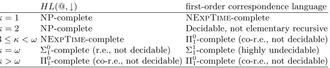
Table 1: Complexity of the satisfiability problem onκ-models
HL(@,↓) first-order correspondence language
κ= 1 NP-complete NExpTime-complete
κ= 2 NP-complete Decidable, not elementary recursive
3≤κ < ωNExpTime-complete Π0
1-complete (co-r.e., not decidable)
κ=ω Σ0
1-complete (r.e., not decidable) Σ11-complete (highly undecidable)
κ > ω Π0
1-complete (co-r.e., not decidable) Π01-complete (co-r.e., not decidable)
a restricted number of points. More precisely, for any cardinalκ, letKκ be the class of uni-modal models in which for every nodedthere are strictly less than
κnodesesuch that (d, e)∈R. In particular,K2is the class of models in which
every points has at most oneR-successor, andKωis the class of models in which every node has only finitely manyR-successors. We will refer to elements ofKκ asκ-models for short. In what follows we will consider the satisfiability problem of HL(@,↓) and of the first-order correspondence language on κ-models, for particularκ. Our results are summarized in Table 1. All results generalize to to case with multiple modalities, except for the decidability of the first-order correspondence language onK2.
The terminology and results used in this section can be found in [8] and [17], or in other texts on computational complexity. In particular, we follow the usual terminology from recursion theory: the language of second-order arithmetic is the second-order language with constants 0, 1, function symbols + and×, and equality. Formulas of second-order arithmetic are interpreted over the natural numbers. A Σ1
1 formula of second order arithmetic is a formula of the form
∃R1. . . Rn.φwhere φcontains no second-order quantifiers. A set A of natural numbers is said to be in Σ1
1if it is defined by a Σ11formula that has one free
first-order variable and no free second-first-order variables. A setAof natural numbers is Σ1
1-hard if for everyBin Σ11there is a computable functionf :N→Nsuch that
for alln∈N,n∈B ifff(n)∈A. A set of natural numbers is Σ11-complete if it is both in Σ1
1and Σ11-hard. It is well known that Σ11-hard sets are not recursively
enumerable. When one speaks of an arbitrary decision problem as being in Σ1 1
or Σ11-hard, it is implicitly understood that the instances of the decision problem
are coded into natural numbers (under some computable encoding).
Following [8], we call a decidable problem elementary recursive if the time complexity can be bounded by a constant number of iterations of the exponential function.
Finally, given a formula φ and a unary predicateP, we will use the nota-tionφP to refer to the relativisation of φ by P, i.e., the result of replacing all subformulas inφof the form∃x.ψ or ∀x.ψ by∃x.(P x∧ψ) resp.∀x.(P x→ψ).
Theorem 5.1 The satisfiability problem ofHL(@,↓)on the class of modelsKκ is
2. NExpTime-complete, for 3≤κ < ω.
3. Recursively enumerable but not decidable, for κ=ω
4. Co-recursively enumerable but not decidable, for κ > ω
Proof.
1. The lower bound follows from the NP-hardness of propositional satisfi-ability. The upper bound is proved by establishing the polynomial size model property.
For κ = 1,2, every κ-satisfiable HL(@,↓)-formula is satisfiable in a κ -model with at most O(|φ|2) nodes. For, suppose M, w |= φ for some
κ-model M = (W, R, V). Let W0 ⊆ W consist of all worlds that are
reachable fromwor from a world named by one of the nominals occurring in φin at most md(φ) steps, wheremd(φ) is the modal depth of φ. Let
M0be the submodel ofMwith domainW0. Clearly,M0 is aκ-model and M0 satisfies the cardinality requirements. Furthermore, a straightforward
induction argument shows thatM0, w|=φ.
This leads to a non-deterministic polynomial time algorithm for testing satisfiability of an HL(@,↓)-formula φ on κ-models, for κ = 1,2. The algorithm first non-deterministically chooses a candidate model (M, w) of
size O(|φ|2), and then it tests whether M, w |= φ and M ∈ Kκ. The
latter tests can be performed in polynomial time using a top down model checking algorithm (cf. Theorem 6.1 below).
2. [Upper bound]For 3≤κ < ω, every formula satisfiable on aκ-model is satisfiable on aκ-model with at mostO(|φ| ·κmd(φ)) nodes. For, suppose
M, w |=φfor some κ-model M= (W, R, V). Let W0 ⊆W consist of all
worlds that are reachable from w or from a world named by one of the nominals occurring inφin at mostmd(φ) steps. LetM0 be the submodel
ofMwith domainW0. Note that the cardinality ofM0isO(|φ| ·κ|φ|), and M0is still aκ-model. Furthermore, a straightforward induction argument
shows thatM0, w|=φ.
This leads to a non-deterministic ExpTime algorithm for testing satisfi-ability of an HL(@,↓)-formulaφ on κ-models. The algorithm first non-deterministically chooses a candidate model (M, w) of size O(|φ| ·κ|φ|),
and then tests whether M, w |=φ. The latter test can be performed in
timeO(|M||φ|) [13], which isO((|φ| ·κ|φ|)|φ|) =O(|φ||φ|·κ(|φ|2)
).
Fix a nominali, and for any monadic first-order formulaφwithout equal-ity, defineφ+ inductively, such that (x=y)+= @xy, (P x)+= @xp, (·)+
commutes with the Boolean connectives and (∃x.ψ)+ = @i3|φ|↓x.ψ. In words, φ+ states that φ holds in the submodel consisting of all points
reachable from the point namedi in exactly|φ| many steps. In general, there can be up to (κ−1)|φ|many points reachable from the point named
iin exactly|φ|many steps (in particular, this will be the case if the sub-model generated byiis a (κ−1)-ary tree). It follows thatφis satisfiable iffφ is satisfiable in a model with at most 2|φ| nodes iff φ+ is satisfiable in aκ-model, for κ≥3.
3. We will provide polynomial reductions between this problem and the finite satisfiability problem for first-order logic. The satisfiability problem for first-order logic on finite models is Σ0
1-complete, even in the case with only
a single, binary relation [8, Section 3.2].
Trivially, if an HL(@,↓)-formula is satisfiable in a finite model, it in a
ω-model. Conversely, if anHL(@,↓)-formula is satisfiable in anω-model then is satisfiable in a finite model, since the modal depth of the formula provides a bound on the depth of the model. Hence, the satisfiability problem ofHL(@,↓) onω-models reduces (by the Standard Translation) to the satisfiability problem for first-order logic on finite models.
Conversely, the finite satisfiability problem for first-order logic can be reduced to satisfiability of HL(@,↓) on ω-models. Fix a nominal i, and for any first-order formulaφ, defineφ+inductively, such that (x=y)+= @xy, (Rxy)+ = @x3y, (·)+ commutes with the Boolean connectives and
(∃x.ψ)+= @i3↓x.ψ+. In words, φ+ states thatφholds in the submodel
consisting of the successors of the point named i. It follows that φ is satisfiable in a finite model iff theHL(@,↓)-formulaφ+ is satisfiable on
an finitely branchingω-model.
4. By the L¨owenheim-Skolem theorem, a first-order formula is satisfiable if and only if it is satisfiable on a finite or countably infinite model. Since
HL(@,↓) is a fragment of first-order logic, the L¨owenheim-Skolem theorem also applies toHL(@,↓)-formulas. It follows that the satisfiability problem for HL(@,↓) on countably branching models coincides with the general satisfiability problem ofHL(@,↓), which is Π0
1 complete by Theorem 3.1.
qed
Theorem 5.2 The satisfiability problem of first-order sentences of the corre-spondence language onKκ is
1. NExpTime complete, for κ= 1
2. decidable but not elementary recursive, forκ= 2
4. Σ1
1-hard, and hence neither recursively enumerable nor co-recursively
enu-merable, for κ=ω
5. Co-recursively enumerable but not decidable, for κ > ω
Proof.
1. This case coincides with the satisfiability problem for monadic first-order logic (on 1-models, every formula of the form Rst is equivalent to ⊥), which is known to beNExpTimecomplete [8].
2. Consider the satisfiability problem for first-order logic with one unary function symbol, an arbitrary number of unary relation symbols and equal-ity (“the Rabin class”). This problem is decidable, but not elementary recursive [8]. We will provide reductions between this problem and the satisfiability problem for first-order logic on 2-models.
• Letφbe any first-order formula containing one unary function symbol
f and any number of unary relation symbols and equality. LetRbe a binary relation symbol, and letφRbe obtained fromφby repeatedly applying the rewrite rules
– replace atomic formulas of the formP f(t) by∃x.(Rtx∧P x) – replace atomic formulas of the form f(s) = t or t = f(s) by
∃x.(Rsx∧x=t)
until the function symbol f does not occur in the formula anymore (in case of nested function symbols, the above rules might need to be applied several times). It is not hard to see thatφis satisfiable iff
φR∧ ∀x∃y.Rxy is satisfiable on a 2-model.
• Let φ be any first-order formula with one binary relation symbol
R and any number of unary relation symbols. Let f be a unary function symbol and letP be a new unary relation, and letφf be the result of replacing all subformulas ofφof the formRstbyP s∧(t=
f s). Intuitively, the unary predicateP represents the existence of a successor, and the unary functionf encodes the successor of a node, if it exists. One can easily see that φis satisfiable on a 2-model iff
φf is satisfiable (simply letRdenote the graph off, or vice versa).
It follows that the satisfiability problem of first-order logic on 2-models is decidable but not elementary recursive.
3. It is known that the satisfiability problem for first-order sentences with a single binary relation R is Π0
1-complete [8]. For any such first-order
formulaφdefineφ∗ as follows:
(x=y)∗ = x=y
(Rxy)∗ = ∃x0y0.(¬Rx0x0∧ ¬Ry0y0∧Rx0y0∧Rx0x∧Ry0y) (¬φ)∗ = ¬φ∗
We claim that φ is satisfiable in a model Miff φ∗ is satisfiable on a
3-model M0. Intuitively, the reflexive nodes of M0 will correspond to the
nodes of M, and the irreflexive nodes of M0 will be used to encode the
binary relation ofM: we think of reflexive pointsd, e as standing in the
binary relation iff there are irreflexive points d0, e0 such that (d0, d)∈ R, (d0, e0)∈R and (e0, e)∈R. More precisely, the argument can be spelled out as follows.
[⇒] Suppose M |= φ, with M = (D, R). Let D0 be a set of objects obtained fromDby adding by adding new objects (d, e)1 and (d, e)2
for all d, e ∈ D. Let R0 ={(d, d),((d, e)
1, d),((d, e)2, d)| d∈ D} ∪
{((d, e)1,(d, e)2)|(d, e)∈R}. The model (D0, R0) is a 3-model, and
by induction on can easily show thatM0 |=φ∗.
[⇐] Suppose M|=φ∗ for some 3-modelM= (D, I). Let D0 ={d∈D|
(d, d) ∈ R}. Let R0 = {(d, e) ∈ (D0)2 | (d0, d0) 6∈ R and (e0, e0) 6∈
Rand (d0, d)∈ R and (e0, e)∈ R and (d0, e0)∈ R, for somed0, e0 ∈
D}. Let M0 = (D0, R0). A straightforward induction shows that M0|=φ.
For 3 < κ < ω, it follows that a first-order formulas φ with one binary relation R is satisfiable iff φ∗∧ ∀x∃≤2y.Rxy is satisfiable on a κ-model.
Hence, satisfiability of first-order formulas on κ-models is Π0
1-hard.
Fi-nally, membership of Π0
1follows from the fact that the satisfiability
prob-lem for first-order formulas is in Π01, sinceφis satisfiable on aκ-model iff
φ∧ ∀x∃≤κy.Rxy is satisfiable.
4. We will provide reductions between that the satisfiability problem for first-order formulas onω-models and the problem of deciding whether an exis-tential second order sentence holds in the model (N, <). This proves the result, since the latter problem is Σ1
1-complete [9].
Let φ(N,>) be a first-order sentence expressing that R is a strict linear
order and ∀x∃y.Ryx. Then a finitely branching model satisfies φ(N,>)
precisely if the model is isomorphic to (N, >). For any existential second order sentenceφ=∃R1. . . Rn.ψ(R1, . . . , Rn, >), let φ∗ be the defined as follows, whereP1, . . . , Pn, N are new, distinct unary predicates.
(x=y)∗ = x=y (x > y)∗ = Rxy (Rkx1. . . xn)∗ = ∃y1. . . yn.
¡ V
m=1...n(Pkym∧Rymxm)∧ V
m=1...n−1(Rymym+1)¢
(¬φ)∗ = ¬φ∗ (φ∧ψ)∗ = φ∗∧ψ∗ (∃x.φ)∗ = ∃x(N x∧φ∗)
We claim that (N, >)|=φiffφ∗∧φN
(N,>)is satisfiable in a finitely branching
model, whereφN
N. This can be seem as follows. The submodel consisting of the points satisfying N is the “intended model”, while the elements satisfying one of the unary predicatesPk are only used to encode which tuples stand in theRk relation. More specifically, a tuple (d1, . . . , dn) of points satisfying
N is thought to stand in the Rk relation iff there are points e1, . . . , en satisfyingPksuch thatemRdmfor allm≤nandemRem+1for allm < n.
We will omit the details of the proof here.
Now for the other direction. First, observe that whenever a first-order formula has a finitely branching model M, then it has a countable such
model (indeed, it suffices to take any countable elementary submodel of
M). Now, for any first-order formulaφ(R, P1, . . . , Pn), letφ0 be the
exis-tential second order sentence∃R, P1, . . . , Pn.(φ∧ ∀x∃y∀z.(Rxz→z < y)). Observe how, on the natural numbers, the second conjunct enforces that each point has only finite manyR-successors). It follows that φis satis-fiable in a countableω-model iffφ0 is true in a submodel of (N, <). The latter in turn holds iff∃Q.(φ0)Q is true in (N, <), where (φ0)Qis the result of relativising all quantifiers inφ0 byQ.
5. By the L¨owenheim-Skolem theorem, a first-order formula is satisfiable if and only if it is satisfiable on a finite or countably infinite model. Hence, the satisfiability problem on countably branching models coincides with the general satisfiability problem, which is known to be Π0
1-complete [8].
qed
6
Model checking
So far, we only studied the satisfiability and the validity problems. It is natural to ask how our syntactic and semantic restrictions affect the complexity of the model checking problem.
Given a hybrid modelM, an assignmentg, a statew, and a hybrid formula
α, themodel checking problem is to check whetherM, g, w²α. We will restrict ourselves to hybrid sentences. This is not a limitation, since we can always replace a free variablexby a fresh nominalix such that the valuation V ofix is the state associated toxby the assignmentg.
In [13], the authors give a polynomial time model checker forHL(@,3−, E). Moreover, they prove that the model checking problem forHL(@,↓) isPSpace -complete, as is the case for the full first-order correspondence language. This result holds even for formulas without @, nominals, and propositions.
Theorem 6.1 The model checking problem for HL(@,↓) on κ-models can be solved in polynomial time forκ≤2, and is PSpace-complete for κ≥3.
As for the second part, the proof of PSpace-hardness of model checking for
HL(@,↓) given in [13] uses a model with out-degree 2. It follows that the model checking problem forHL(@,↓) onκ-models, withκ≥3, isPSpace-complete.
qed
On the contrary, model checking forHL(@, E,↓) and for first-order logic is
PSpace-complete even on 1-models [13].
In the following, we investigate how to restrict the syntax of hybrid languages in order to lower down the complexity of model checking. A first result is that, if formulas do not show the↓2↓pattern, then the model checking problem drops fromPSpace-complete to NP-complete.
Theorem 6.2 The model checking problem forF HL\ ↓2↓is NP-complete.
Proof. To proveNP-hardness, we embed the satisfiability problem for propo-sitional formulas (SAT) into the model checking problem for HL\ ↓2↓. Let
φ(p1, . . . , pn) be any propositional formula, and let M = (W, R, V), where
W ={0,1},R=W×W. For eachpkoccurring inφ, pick a corresponding state variablexk. Furthermore, lety be a state variable distinct from allx1, . . . , xn.
Letφ0 be obtained fromφby replacing each occurrence ofp
k by3(xk∧y), for
k = 1. . . n. Intuitively, the two states of M represent truth and falsity, and among these two states the variabley denotes the truth state. It is easily seen that the propositional formula φ is satisfiable iff 3↓y3↓x13↓x2. . .3↓xn.φ0 is true inM (at any of the nodes 0,1). The latter formula contains no2operators, and hence belongs toF HL\ ↓2↓.
To prove membership of NP, we give a nondeterministic algorithm that solves the model checking problem in polynomial time. Letαbe anF HL\ ↓2↓
sentence,M = (W, R, V) be a model andv∈W. Replace each subformula ofα
of the form↓x.ϕby∃x.(x ∧ ϕ), and apply the equivalences given in the proof of Theorem 4.1 in order to move the existential quantifiers out of the scope of as many connectives as possible. The resulting sentenceα0 is equivalent toα and has the following properties:
1. α0 is built up from literals (i.e., formulas of the form (¬)p, (¬)ior (¬)x) using conjunction, disjunction, existential operators (3,3−, E), universal operators (2,2−, A) and existential quantifiers.
2. All existential quantifiers in α0 either immediately follow a universal op-erator (e.g., as in2∃x1. . . xnβ) or occur at the start of the formula.
3. For all subformulas of α0 of the form X∃x
1. . . xnβ, with X a universal operator,β contains no free variables besidesx1, . . . , xn.
List all subformulas of α0 of the form Xβ, with X a universal operator and
β=∃x1. . .∃xm.γ(x1. . . xm), in order of increasing length, and do the following
Create a new proposition symbolpβ and replaceβ bypβ inα0. For each state w ∈ W, check whether M, w ² β, and if so, insert the statewinV(pβ).
Finally, apply the usual model checking algorithm to check if in polynomial time ifv satisfies the resultingHL(@,3−, E) formula. If so, return true, else return false.
The nondeterminism is hidden in the test M, w ² β in step 3. To check
M, w²∃x1. . .∃xm.γ(x1. . . xm), the algorithm guesses an assignment gfor the
variables x1, . . . , xn and checks whether M, g, w ² γ(x1. . . xm). Since γ does
not contain any existential quantifiers (the subformulas were processed in order of increasing length), it belongs to HL(@,3−, E). Hence, the check whether
M, g, w|=γcan be performed in polynomial time. All in all, our model checking algorithm runs in nondeterministic polynomial time. qed
Notice that theNP-hardness holds even for formulas without proposition letters, nominals and @-operators. Also note that bothF HL\2↓ andF HL\ ↓2 are subsets of F HL\ ↓2↓. Hence, the model checking for both F HL\2↓ and
F HL\↓2isNP-complete. A typical example of a formula to which Theorem 6.2 does not apply is↓x.22↓y.@x3y, which expresses a local form of transitivity.
In Section 4, we saw thatF HL\2↓2has a decidable satisfiability problem. We leave it as an open question whether the model checking complexity of that fragment also belowPSpace(since the SAT problem can be embedded into the model checking problem forF HL\2↓2as done in the proof of Theorem 6.2, the problem is at least NP-hard). Conversely, the fragment F HL\ ↓2↓ for which we have just proved that the model checking problem isNP-complete, has an undecidable satisfiability problem: it suffices to note that the encoding of the tiling problem given in Section 3 does not make use of↓2↓-formulas.
We conclude this section with a hierarchy of fragments of the full hybrid language with ↓ binder that admits polynomial time model checking. As we remarked already in Section 2, if a hybrid formulaαhas widthw, thenSTx(α) has width at mostw+ 2. Hence, a bound on the width of the hybrid formulas implies a bound on the width of the standard translations. Moreover, model checking for first-order formulas using a bounded number of variables can be performed in polynomial time [21]. It is known that first-order formulas of a bounded width can be rewritten using a bounded number of variables (cf. [11] for an explicit proof). Thus, we obtain the following.
Theorem 6.3 The model checking problem for formulas of the full hybrid lan-guage of bounded width can be solved in polynomial time.
Proof. LetM be a hybrid model withn nodes andαbe a formula of length
kand widthw. Applying the Standard Translation toα, we obtainSTx(α), a first-order formula with width at mostw+ 2. The Standard Translation can be implemented in linear timeO(k). Each first-order formula of width w can be translated in quadratic timeO(k2) into a formula using at mostwvariables [11].
on a model ofnnodes costsO(k·nv) [21]. Hence, we can model checkαin time
O(k2+k·nw+2). This is polynomial since wis constant. qed
Notice that a formula of bounded width can use an arbitrary number of variables and can have an arbitrary nesting degree of↓. For instance, let α0=
x1, and, forn >0, letαn =E↓xn.(3xn+1 ∧αn−1). For n >0, the formulaαn says that there are pointsx1, . . . , xn+1such thatxireachesxi+1fori= 1, . . . , n.
It is easy to see that, forn >0, the width ofαn is 2. Moreover,αn usesn+ 1 variables and the nesting degree of↓ inαn isn.
7
Conclusion
In this paper, we described two ways to tame the hybrid logicHL(@,↓), and in fact the full hybrid languageHL(@, E,↓,3−). By taming a logic we mean restricting it in such a way that it becomes decidable. These two ways are:
1. Restricting the syntax by excluding formulas containing the pattern2↓2.
2. Restricting the class of models by assuming a bound on the branching degree of the models.
Furthermore, we showed that similar restrictions can be used to lower the complexity of model checking task for these logics.
Some results in this paper show that, under certain natural conditions,
H(@,↓) behaves better than the first-order correspondence language, compu-tationally speaking. Incidentally, the full hybrid languageHL(@, E,↓,3−) has the same expressive power as the full first-order correspondence language, as is shown by the following translation [5]:
HT(x=y) = @xy HT(P x) = @xp HT(Rxy) = @x3y HT(¬φ) = ¬HT(φ)
HT(φ∧ψ) = HT(φ)∧HT(ψ)
HT(∃x.φ) = E↓x.HT(φ)
The last clause of this translation shows that, in some sense, the first-order quantifier∃xconsist of two parts, namely thepicking a state of the model part, which is captured by the global modality, and thevariable binding part, which is captured by the ↓. The syntax of HL(@, E,↓,3−) allows us to distinguish these two parts. Hence, one could say that some of our results identify compu-tationally tractable fragments of first-order logic that can only be distinguished once these two parts of the quantifiers are split. In this sense, our paper can be seen as a fine study of the structure of first-order quantifiers.
for a sequence of universal resp. existential operators), one could consider the fragment F HL\σ. Then it follows from the undecidability proof by tiling in Section 3 that there is no such sequenceσ that contains 2↓2 as a proper subsequence and such thatF HL\σis decidable. In other words, our decidability result is optimal.
Finally, the outcomes of our investigation show once more that, from a com-putational point of view, the satisfiability problem and the model checking prob-lem for a logic are sensitive to different sources of complexity. Restricting the width (i.e., the out-degree) of the model makes the satisfiability problem de-cidable, but it does not lower the complexity of the model checking problem (unless the width is less than two). On the other hand, restricting the width of the formula makes the model checking problem more tractable, but it does not affect the undecidability of the satisfiability problem (unless the width is 0).
References
[1] H. Andr´eka, J. van Benthem, and I. N´emeti. Modal logics and bounded fragments of predicate logic. Journal of Philosophical Logic, 27(3):217–274, 1998.
[2] C. Areces, P. Blackburn, and M. Marx. A road-map on complexity for hybrid logics. In J. Flum and M. Rodr´ıguez Artalejo, editors,Proceedings of the 8th Annual Conference of the EACSL, Madrid, 1999.
[3] C. Areces, P. Blackburn, and M. Marx. The computational complexity of hybrid temporal logics. Logic Journal of the IGPL, 8(5):653–679, 2000.
[4] C. Areces, P. Blackburn, and M. Marx. Hybrid logics: Characterization, interpolation, and complexity. Journal of Symbolic Logic, 66(3):977–1010, 2001.
[5] P. Blackburn. Representation, reasoning, and relational structures: A hy-brid logic manifesto. Logic Journal of the IGPL, 8(3):339–365, 2000.
[6] P. Blackburn, M. de Rijke, and Y. Venema. Modal Logic. Cambridge University Press, 2001.
[7] P. Blackburn and J. Seligman. Hybrid languages. Journal of Logic, Lan-guage and Information, 4:251–272, 1995.
[8] E. B¨orger, E. Gr¨adel, and Y. Gurevich. The Classical Decision Problem. Springer, Berlin, 1997.
[9] B. ten Cate. Model theory for Extended Modal Languages. PhD thesis, ILLC, University of Amsterdam, 2005.
[10] B. ten Cate. Interpolation for extended modal languages. Journal of Symbolic Logic, To appear. A preliminary version is available from
[11] B. ten Cate and M. Franceschet. Guarded fragments with constants. Tech-nical Report PP-2004-32, ILLC, University of Amsterdam, 2004.
[12] M. Fisher and R. Ladner. Propositional dynamic logic of regular programs. Journal of Computer and System Sciences, 18(2):194–211, 1979.
[13] M. Franceschet and M. de Rijke. Model checking for hybrid logics. In Proceedings of the Workshop Methods for Modalities, 2003.
[14] V. Goranko. Hierarchies of modal and temporal logics with reference point-ers. Journal of Logic, Language, and Information, 5(1):1–24, 1996.
[15] E. Gr¨adel. On the restraining power of guards. Journal of Symbolic Logic, 64:1719–1742, 1999.
[16] E. Gr¨adel and M. Otto. On logics with two variables.Theoretical computer science, 224(1-2):73–113, 1999.
[17] D. Harel. Recurring dominoes: making the highly undecidable highly un-derstandable. Annals of Discrete Mathematics, 24:51–72, 1985.
[18] E. Hoogland. Definability and Interpolation. PhD thesis, University of Amsterdam, 2001.
[19] M. Marx. Narcissists, stepmothers and spies. InProceedings of the Inter-national Workshop on Description Logics, 2002.
[20] M. Mortimer. On languages with two variables. Zeitschrift f¨ur mathema-tische Logik und Grundlagen der Mathematik, 21:135–140, 1975.