Programming with Classical Proofs
MSc Thesis(Afstudeerscriptie) written by
Hans Bugge Grathwohl
(born January 10th 1989 in Frederiksberg, Denmark)
under the supervision of prof. dr. Herman Geuvers and dr. Inge Bethke, and submitted to the Board of Examiners in partial fulfillment of
the requirements for the degree of
MSc in Logic
at theUniversiteit van Amsterdam.
Date of the public defense: Members of the Thesis Committee:
August 27th 2013 dr. Maria Aloni
prof. dr. Herman Geuvers dr. Inge Bethke
i
Abstract
This thesis is about extracting programs from classical proofs. In the first part, we show conservativity of Peano arithmetic over Heyting arithmetic for Π02-sentences, an old result of Kreisel, using Friedman’s
A-translation technique. Then we present some extensions by Parigot and Krebbers of the lambda-calculus with control mechanisms, that allow for some amount of classical reasoning via the Curry–Howard correspondence.
In the second part of the thesis, we present a new system by Aschieri and Berardi,HA+EM1, a Curry–Howard system for an arithmetic with
a limited amount of classical reasoning that is based on ideas from their Interactive Realizability semantics for classical arithmetic. We show Aschieri’s recent proof of strong normalization ofHA+EM1that uses a
new technique based on non-deterministic choice.
iii
Acknowledgements
I would like to thank my supervisor Herman Geuvers for introducing me to the area of classical program extraction, and for a lot of good, fruitful meetings in Nijmegen. Furthermore, I would like to thank Inge Bethke for being willing to take up the job as my local supervisor.
I am grateful to my brother Bjørn, the computer scientist, who has carefully read my drafts and provided valuable comments and corrections.
Contents
1 Introduction 1
1.1 Related work . . . 2
1.2 Outline . . . 3
1.3 Notation . . . 4
2 Preliminaries 5 2.1 Natural deduction . . . 5
2.2 First-order logic . . . 6
2.3 The untyped lambda calculus . . . 9
2.4 Simply typed lambda calculus . . . 11
2.5 G¨odel’s System T. . . 13
2.6 Annotated first-order proofs . . . 16
3 Friedman’s A-translation 19 3.1 The arithmeticsPAand HA . . . 19
3.2 Double-negation translation . . . 20
3.3 A-translation . . . 22
3.4 The proof . . . 24
4 Control operators 27 4.1 The systemλµ . . . 28
4.2 The systemλµT . . . 31
5 Arithmetic with exceptions: HA+EM1 35 5.1 Post rules . . . 35
5.2 HA . . . 37
5.3 HA+EM1 . . . 41
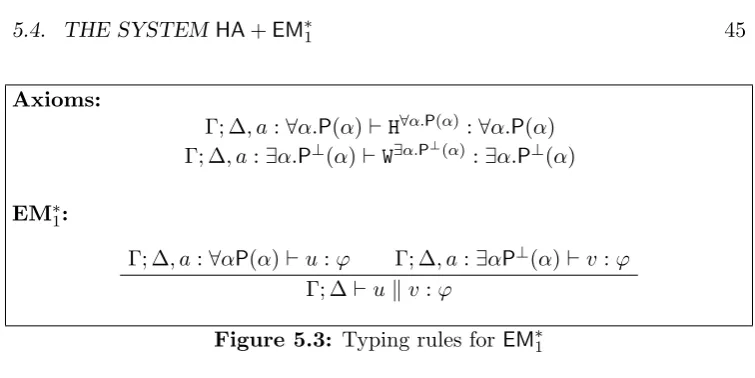
5.4 The systemHA+EM∗1 . . . 45
5.5 Strong normalization forHA+EM∗1 and HA+EM1 . . . 47
5.6 Existential witness property . . . 54
6 Programming with terms in HA+EM1 55 6.1 Searching . . . 55
6.2 Multiplication example . . . 61
7 Program extraction from HA+EM1 67
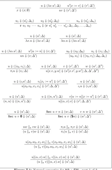
7.1 Natural semantics for HA+EM1 . . . 67
7.2 Searching . . . 70 7.3 Multiplication . . . 71
8 Conclusion 73
8.1 Further research . . . 73
Chapter 1
Introduction
A fundamental result about the theory of computer programming is Rice’s theorem, which states that there is no effective way of deciding whether an algorithm computes a partial recursive function with a given non-trivial property. A consequence of this is, that it is in general undecidable whether a given program meets its specification. One approach to solve this problem stems from a combination of two observations: Firstly, that there is a tight connection between computer programs and proofs, this is what is commonly known as theCurry–Howard correspondence, sometimes referred to as proofs-as-programs and formulas-as-types. Secondly, the observation that it is decidable whether a formal proof is correct. Thus, the idea is to make a mathematical proof of a specification (which, of course, might be hard), and from this extract a correct computer program. This is what is known as program extraction. It is well established that this method works well when we consider intuitionistic proof systems. Paulin-Mohring, e.g., in [32] presented a method to extract correct programs from proofs in the Calculus of Construction, a higher order λ -calculus with dependent types [12]. In [29], Parigot discusses the practicalities of the idea of programming with proofs, i.e., using formal mathematics as a programming language.
This method needs the proofs to be constructive, in the sense that from a proof of an existential statement, one can get a witness of this statement. All proofs in intuitionistic logic are constructive, and indeed, for people working in program extraction, attention was in the beginning restricted to intuitionistic logics. Classical logics are not constructive in the same sense, and thus it does not a priori seem to be possible to apply the same techniques here. However, an old result about arithmetic states that any Π02-sentence is provable in Peano arithmetic if and only if it is provable in Heyting arithmetic. Thus, there is a method to transform any classical proof of a specification in arithmetic, i.e., a proof of ∀α∃β.P(α, β) whereP(α, β) is a basic formula, into an intuitionistic proof of the same specification. This is evidence that all classical proofs of Π02 -sentences have some computational content. Π0
2-sentences are indeed arguably
the most important sentences in computer science, since a proof of one of these corresponds to a proof of totality of a recursive function. This leads to the area ofclassical program extraction.
There have been several approaches to extracting the computational content of these classical proofs. It was discovered by Griffin in 1989 [20] that inference by contradiction corresponds to Felleisen’s control operatorC [13], and hence the Curry–Howard correspondence was extended to include classical reasoning. This sparked a lot of research in this area. Several extensions of theλ-calculus with control operators have been proposed. To name a couple: Felleisen’s λC with typing rules by Griffin; Rehof and Sørensen’s λ∆ [36] that extends
ordinaryλ-terms with a binder ∆ which is typed byreductio ad absurdum; and Parigot’s λµ[30], which we will return to in Chapter 4, along with Krebbers’s λµT which extends λµ with natural numbers as a primitive datatype.
These systems correspond to classicalpropositional logic, which means that their type systems are rather simple, and that, when they are equipped with datatypes, they are more closely related to real world computer programming languages than first-order systems are. But since we are interested in proofs of statements of the form ∀α∃β.ϕ(α, β), we need to consider systems that correspond to first-order logic. For intuitionistic logic the standard system is IQC, and when this is extended with the Peano axioms for arithmetic, we get Heyting arithmetic, HA. In HAwe do not need to add datatypes, since the natural numbers are primitive in it. In this thesis we are mainly concerned with an extension ofHAwith a limited amount of classical reasoning in the form ofEM1, the law of excluded middle restricted to Σ01-formulas. The system
HA+EM1 that we present in Chapter 5 is a very recent system by Aschieri and
Berardi, and therefore it is not yet well studied. We work out some non-trivial proofs in this system, and discuss how we can extract programs from these.
1.1
Related work
Berger, Buchholz, and Schwichtenberg [11] describe a method for extracting programs from classical proofs, by way of extracting a term in G¨odel’s System T which contains all the computationally relevant parts of the proof. This is in the style of the G¨odel–Gentzen double negation translation, and indeed the target language does not contain control mechanisms.
In [28], Makarov utilizes Felleisen’sC-operator to extract a program from a classical proof of a non-trivial arithmetical proposition by adding extra inference rules and defining a structural operational semantics for the classical deduction system.
1.2. OUTLINE 3
Krebbers extended Parigot’sλµ to contain a primitive datatype for the natural numbers, in the style of G¨odel’s System T, so as to come closer to “real” programming languages, since these all have primitive datatypes. We will present this system in Chapter 4. Furthermore, he has developed λ::catch, which is an extension of Herbelin’s IQCMP-calculus withcatchandthrow[21], this time with lists as a primitive datatype.
Aschieri and Berardi has developedinteractive realizability [2, 4, 5, 7], which is a computational semantics for classical proofs that is based on the principle of learning. Instead of following the method of Avigad [8], who characterizes his classical realizability in terms of a special double-negation translation followed by Friedman’s A-translation, followed by Kreisel’s modified realizability [26], Aschieri avoids the use of a double-negation translation, and instead combines modified realizability and Friedman’s translation. The learning aspect is based on the idea that whenever we use an instance of excluded middle
∀α.ϕ(α)∨ ∃α.¬ϕ(α) in a proof, the realizer starts byassuming that∀α.ϕ(α) is the case, and then whenever we use an instance ϕ(n) in the proof, the realizer checks to see if this is actually the case. The realizer then updates its state with this new information (it learns). If ϕ(n) is the case, then it continues under the assumption that ∀α.ϕ(α) holds, and if not, it has found a witness for ∃α.¬ϕ(α), thus this must hold, and the realizer continues in the part of the proof that work under this assumption.
It is on the basis of interactive realizability that Aschieri and Berardi have developed the classical Curry–Howard system HA+EM1 [3, 6] that we will
investigate in this thesis.
1.2
Outline
In Chapter 2 we present some basic proof theory and lambda calculus, and we introduce some type systems, namely the simply typed lambda calculusλ→,
G¨odel’s System T, and MQC, a calculus for minimal first-order logic.
In Chapter 3 we present a proof of Kreisel’s theorem thatPA is a conserva-tive extension ofHAfor Π02-sentences, via the G¨odel–Gentzen double-negation translation and Friedman’s A-translation, which lays ground to most of the methods employed in the area of classical program extraction.
In Chapter 4 we discuss how to introduce control mechanisms in the λ -calculus, and specifically we present the systems λµ by Parigot, andλµT by Krebbers. These are examples of simple programming languages with control mechanisms that correspond via Curry–Howard to classical logic.
In Chapter 5 we present a systemHA, and expand this to Aschieri’s system HA+EM1. We prove strong normalization ofHA+EM1 by a new method of
Aschieri [3] that uses non-deterministic choice.
In Chapter 6 we investigate how to useHA+EM1for program extraction via
of a searching problem, and the second example is a multiplication program which uses control to increase efficiency.
In Chapter 7 we introduce a new operational semantics forHA+EM1, and
test this on some examples from Chapter 6.
1.3
Notation
We use greek letters,α, β, γ, . . . to refer to numeric variable, lettersx, y, z, . . . to refer to proof variables, and lettersa, b, c, . . . to refer to variables that acts as “addresses” for control mechanisms. For proof terms, we will mainly use the lettersu, v, w, . . ., and for numeric terms we will mostly usen, m, . . ..
When writingλ-abstractions, we will often omit the annotated types, even if we are working in Church-style. This saves space, and the types can be deduced from the context.
For formulasϕ, we will often writeϕ(α), which means that we can substitute α withn simply by writingϕ(n). It does not necessarily imply that α is the only free variable inϕ.
Natural deduction proof trees are defined with a turnstile and an environ-ment, Γ, and`, but since this makes the, already bulky, trees look even more voluminous, we will often discharge variables with superscripts instead:
τ `τ
`τ →τ versus
Chapter 2
Preliminaries
2.1
Natural deduction
We first define what a natural deduction system is in general.
Definition 2.1.1 (Natural deduction systems). Let L be a language. We define a natural deduction system N.
1. An environment in natural deduction is a finite set of formulas of L, usually written Γ.
2. A natural deductionjudgment is a pair consisting of an environment and a formula, written Γ`ϕ. We do not write set-brackets when we specify the environment, thus we write ϕ, ψ`θ instead of {ϕ, ψ} `θ and`ϕ when the environment is empty.
3. An n-ary rule of inference consists of n+ 1 judgments (npremises and one conclusion), and is written on the form
Γ1`ϕ1 Γ2 `ϕ2 · · · Γn`ϕn
Γ`ϕ
A nullary inference rule is called anaxiom. Different natural deduction systems are distinguished by having different inference rules.
4. A proof (synonym: derivation) of a judgment Γ ` ϕ is a finite tree, where:
• Γ`ϕis the root label,
• any label is obtained by its children’s labels by an application of one of the natural deduction rules. If a label is obtained by an application of a nullary rule (an axiom), then it is a leaf.
In general, we will write Γ`ϕto mean that there is a derivation of the judgmentΓ`ϕ. As we will sometimes use multiple natural deduction systems, it can be practical to annotate which system we are using, like so: Γ`N ϕ. Mostly, this will be clear from the context.
2.2
First-order logic
In order to formalize first-order logic, we start by defining a natural deduction proof system for the so-called minimal first-order logic (mFOL). Minimal logic, introduced in 1936 by Ingebrigt Johansson [23], is a simplified version of intuitionistic logic whereex falso quodlibet does not hold. In fact, minimal logic does not contain any rules about absurdity, and therefore⊥ does not need to be in the language. Since negation is usually defined as¬A:=A→ ⊥, we do not necessarily have negation in mFOL.
Firstly, we need to specify what language we work with.
Definition 2.2.1 (The language of first-order logic). Given a signature S
consisting of functional symbols and relational symbols together with their arity, we define the first-order languageLS:
• LetV be a set of distinct variable namesα, β, γ, . . .
• We define theterms of LS as the least setT such that
– V ⊆ T;
– If t1, . . . , tn ∈ T, then f(t1, . . . , tn)∈ T where f is ann-ary func-tional symbol fromS.
A term isclosed if it contains no variables. The closed terms are supposed to represent the objects in the domain of discourse.
• We define theformulas ofLS as the least setF such that
– P(t1, . . . , tn)∈ F where P is an n-ary relation symbol fromS, and
t1, . . . , tn∈ T. These are called atomic formulas. – ϕ∧ψ, ϕ∨ψ, ϕ→ψ∈ F,
– ∀α.ϕ,∃α.ϕ∈ F, where α∈ V. We say that the scope of ∀α (∃α) is ϕ, and we say that any occurrence of α inϕis bound.
In the rest of this document, we will use the less cumbersome Backus-Naur notation when we specify syntax, e.g. when we define terms, formulas, types, etc. The above definition of formulas will then look like:
2.2. FIRST-ORDER LOGIC 7
Example 2.2.2. Consider the signatureS ={0,S,+,=}, where 0is a nullary,
S a unary, and + a binary function symbol, and = a binary relation symbol. Examples of terms of the language LS are
SSα, 0+S0, α+β,
and an example of a formula is
∀αSα=α+S0.
Definition 2.2.3 (Free variables). The set of free variables of a term t, FV(t), is defined inductively:
• FV(α) ={α}, where α is a variable;
• FV(f(t1, . . . , tn)) = FV(t1)∪ · · · ∪FV(tn).
Likewise, we inductively define the set of free variables of a formula A, FV(A):
• FV(P(t1, . . . , tn)) = FV(t1)∪ · · · ∪FV(tn);
• FV(ϕ∧ψ) = FV(ϕ)∪FV(ψ);
• FV(ϕ∨ψ) = FV(ϕ)∪FV(ψ);
• FV(ϕ→ψ) = FV(ϕ)∪FV(ψ);
• FV(∀α ϕ) = FV(ϕ)\ {α};
• FV(∃α ϕ) = FV(ϕ)\ {α}.
If Γ is a set of formulas, then FV(Γ) =S
A∈ΓFV(A).
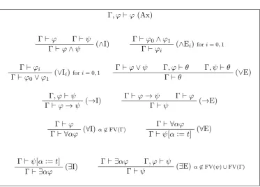
Definition 2.2.4 (mFOL). Given a signatureS, we defineminimal first-order logic (mFOL) overS as the natural deduction system with the inference rule schemata given in Figure 2.1, where all the formulas are from LS.
Intuitionistic and classical logic
To get an intuitionistic first-order logic one needs the ruleex falso quodlibet:
⊥
ϕ
whereϕis any formula and⊥is a symbol forabsurdity. Instead of adding this as a primitive rule, we will later see a method to make this rule admissible, by adding intuitionistic reasoning to the atomic language.
Γ, ϕ`ϕ(Ax)
Γ`ϕ Γ`ψ (∧I) Γ`ϕ∧ψ
Γ`ϕ0∧ϕ1
(∧Ei) fori= 0,1
Γ`ϕi
Γ`ϕi
(∨Ii)fori= 0,1
Γ`ϕ0∨ϕ1
Γ`ϕ∨ψ Γ, ϕ`θ Γ, ψ`θ (∨E) Γ`θ
Γ, ϕ`ψ
(→I) Γ`ϕ→ψ
Γ`ϕ→ψ Γ`ϕ
(→E) Γ`ψ
Γ`ϕ
(∀I) α6∈FV(Γ)
Γ` ∀αϕ
Γ` ∀αϕ
(∀E) Γ`ψ[α:=t]
Γ`ψ[α:=t] (∃I) Γ` ∃αϕ
Γ` ∃αϕ Γ, ϕ`ψ
(∃E)α6∈FV(ψ)∪FV(Γ)
[image:16.595.133.507.113.381.2]Γ`ψ
Figure 2.1: Natural deduction rules for mFOL
• Peirce’s law: We add
Γ`((ϕ→ψ)→ϕ)→ϕ
as an axiomatic rule.
• Reductio ad absurdum: We allow reasoning of the form
[¬ϕ] .. .
⊥
ϕ
which is equivalent to adding ¬¬ϕ→ϕas an axiom.
• Law of excluded middle: We add the axiom
Γ`ϕ∨ ¬ϕ.
2.3. THE UNTYPED LAMBDA CALCULUS 9
Reduction ad absurdum and Peirce’s law have an interesting counter-part in computer programming: Continuation Passing Style programming.
We define the systems iFOL, mcFOL and cFOL, which are simple extensions of mFOL.
Definition 2.2.5 (iFOL). By adding nullary relation symbol⊥ to the signa-ture, and adding the inference rule ex falso quodlibet
Γ` ⊥ (⊥E)
Γ`ϕ
to mFOL, we get intuitionistic first-order logic, iFOL. We definenegation of a formula¬ϕ:=ϕ→ ⊥.
Definition 2.2.6 (mcFOL). By adding thelaw of the excluded middle Γ`ϕ∨ ¬ϕ(EM)
as an axiom schema to mFOL, we get minimal classical first-order logic.
Definition 2.2.7 (cFOL). By adding the law of the excluded middle to iFOL, we getclassical first-order logic.
The systems can be ordered by deductive strength thus:
mFOL ⊂ iFOL
∩ ∩
mcFOL ⊂ cFOL
It is well-known that iFOL is sound and complete with respect to Heyting semantics, and that cFOL is sound and complete with respect to Tarskian semantics.
2.3
The untyped lambda calculus
We give a brief introduction to the untyped lambda calculus, mainly following [9].
Definition 2.3.1 (Untyped λ-terms). We will work with an infinite set of λ-variablesx, y, z, . . .. The untypedλ-terms are defined as follows:
Definition 2.3.2 (Free variables). We define the set of free variables of a λ-term t, FV(t), by induction as follows.
• FV(x) ={x}, when x is aλ-variable;
• FV(ts) = FV(t)∪FV(s);
• FV(λx.t) = FV(t)\ {x}.
A termtis said to beclosed if FV(t) =∅, and otherwise it isopen. If a variable xoccurs in a term t, but x6∈FV(t), thenx is bound; in this case it must be under the scope ofλx.
Definition 2.3.3 (Substitution). The substitution of t for x in s, written s[x:=t], is defined as follows:
x[x:=t] = t;
y[x:=t] = y, ifx6=y;
(st)[x:=t] = (s[x:=t])(t[x:=t]); (λx.s)[x:=t] = λx.s;
(λy.s)[x:=t] = λy.s[x:=t], ifx6=y.
It is, in other words, the result of substituting any free occurrence ofx ins witht.
Definition 2.3.4(α-equivalence). Two terms t, sare said to beα-equivalent, t=αs, if they only differ on bound variables, i.e.:
• Ify is neither free nor bound int, then
λx.t=α λy.t[x:=y].
• Ift=α s, then
λx.t=αλx.s, for all variables x,
tr=αsr, and
rt=αrs. for allλ-termsr.
In practice, we will not distinguish between α-equivalent terms. So we will suppress the α-subscript, and, e.g., say λx.x=λy.y.
2.4. SIMPLY TYPED LAMBDA CALCULUS 11
Because of this convention, any substitution will always be capture avoiding, which means that we will avoid problematic substitutions like
(λx.yx)[y:=x] =λx.xx,
since x is both occurring as a bound variable (inλx.yx) and as a free variable (in the substituendum x), hence it does not satisfy the variable convention.
We will follow this variable convention in all the systems that we define in this document.
Remark 2.3.6. Sometimes it can be necessary to do a vacuousλ-abstraction, i.e., an abstraction over a non-occurring variable. Instead of writing λx.t for x6∈FV(t) we will use the notation λ .t.
Definition 2.3.7 (Compatible relations). We say that a relationRonλ-terms is compatible if, for all termst, s, r
• If tRs, thenλx.t R λx.s, for all variables x;
• If tRs, thentrRsr;
• If tRs, thenrtRrs.
The compatible closure of a relation R is the least compatible relationR0 such that R⊆R0.
Definition 2.3.8 (β-reduction). The relation →β is defined as the least compatible relation that satisfies
(λx.t)s→β t[x:=s].
A term of the shape (λx.t)s is called a β-redex (reducible expression). If a term does not contain any β-redexes, then it is said to be inβ-normal form.
2.4
Simply typed lambda calculus
We define asimply typed lambda calculus, λ→. This is the simplest example of
a type theory, and all systems that we will define later will be extensions of λ→.
There are two common ways of presenting simply typed lambda calculus: In Curry style and inChurch style. In the Curry style, we use the untypedλ-terms, and hence the same term can be assigned multiple different types, while in Church style simply typed lambda calculus we annotate every abstractions with a type so as to ensure that every term has a unique type. We will present it in Church style.
Definition 2.4.1 (Simple types). We have a non-empty set of atomic types,
• A ⊆ T;
• Ifσ, τ ∈ T, then σ→τ ∈ T.
Equivalently, we can express the definition of T with BNF-notation thus: The types of λ→ are
σ, τ ::=a |σ→τ,
wherearanges over the atomic types.
Remark 2.4.2. When writing types, we employ association to the right, i.e., instead of writingσ1 →(σ2→σ3), we will writeσ1 →σ2 →σ3.
We will use the following abbreviation
σ0 →τ :=τ
σn+1 →τ :=σ →σn→τ.
Definition 2.4.3(Type environments). Anenvironment in λ→ is a finite set
of pairs of λ-variables and types, such that each variable occurs maximally once. It is typically denoted Γ,∆, and written on the form
Γ =x1 :ϕ1,· · ·, xn:ϕn.
Definition 2.4.4 (λ→-terms). The difference between typed and untyped
λ-terms is that all variables are annotated with a type: The terms in λ→ are
defined as follows:
t, s:=xτ |λxτ.t|ts,
whereτ is a type.
In practice we can often deduce the type of a variable from the context, in these cases we will typically omit the type annotation, but formally they are still there.
Definition 2.4.5 (Type judgments). Atype judgment is a triple consisting of an environment, a term, and a type, written Γ`t:ϕ.
Definition 2.4.6(Type derivation). Atype derivation of a judgment Γ`t:ϕ is a finite tree where:
• Γ`t:ϕ is the root label;
• Any label is obtained by its children’s labels by an application of one of the typing rules from Figure 2.2.
2.5. G ¨ODEL’S SYSTEM T 13
Γ, x:τ `xτ Γ, x:σ`t:τ Γ`λxσ.t:σ →τ
[image:21.595.180.366.622.689.2]Γ`t:σ →τ Γ`s:σ Γ`ts:τ
Figure 2.2: Typing rules for λ→
Theorem 2.4.7 (The Curry–Howard correspondence). If Γ ` t : σ in λ→,
where Γ = x1 : σ1, . . . , xn : σn, then Γ0 ` σ in minimal propositional logic, where Γ0=σ1, . . . , σn.
For a proof, see [37].
2.5
G¨
odel’s System T
G¨odel’s System T(λT) is an extension ofλ→ that adds the natural numbers
as a primitive datatype together with a recursion operator. In the following definition we also add a Boolean datatype for convenience—this is merely syntactic sugar, since we could just as well have used zero and one to correspond to true and false.
Later in this document, we will see the idea behind the transition fromλ→
to λT be applied on other systems. One should see λT as a model of a simple,
yet powerful, computer programming language.
Definition 2.5.1. The types ofλT are
σ, τ ::=N|Bool |σ→τ
Definition 2.5.2. The terms ofλT are defined inductively over an infinite set of typed λ-variables xτ, yσ, . . .
t, u::=c|xτ |tu |λxτ.t
c::=0|S |True |False|Recτ |ifτ
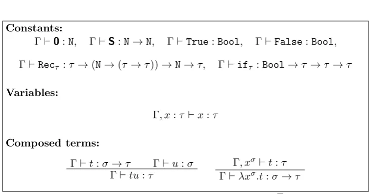
Definition 2.5.3. The typing judgments Γ ` t : σ in λT are given by the typing rules in Figure 2.3.
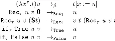
Definition 2.5.4. Reduction,→T, onλT-terms is defined as the compatible
closure of the following reduction rules:
(λxτ.t)u →β t[x:=u] Recτ u v 0 →Rec1 u
Recτ u v (St) →Rec2 v t(Recτ u v t)
ifτ True u v →True u ifτ False u v →False v
As usual, T denotes the transitive and reflexive closure of →T, while =T
Constants:
Γ`0:N, Γ`S:N→N, Γ`True:Bool, Γ`False:Bool,
Γ`Recτ :τ →(N→(τ →τ))→N→τ, Γ`ifτ :Bool→τ →τ →τ
Variables:
Γ, x:τ `x:τ
Composed terms:
Γ`t:σ →τ Γ`u:σ Γ`tu:τ
[image:22.595.130.507.105.303.2]Γ, xσ `t:τ Γ`λxσ.t:σ→τ
Figure 2.3: Typing rules for terms inλT
Definition 2.5.5. A termt is said to be innormal form if tt0 if and only ift≡t0, i.e., t has no possible reductions.
The system λT satisfies the following important meta-theorems:
Theorem 2.5.6. λT satisfies subject reduction: IfΓ`t:σ and tt0, then Γ`t0 :σ.
Proof. It is easy to check that all the reduction rules preserve typing.
Theorem 2.5.7. λT is confluent: Ift1t2 and t1 t3, then there is a term
t4 such thatt2 t4 and t3 t4.
t1
t2 t3
t4
Theorem 2.5.8. λT is strongly normalizing: There are no infinite reduction chains
t1 →t2 →t3 → · · ·
which means that every term has a normal form, and no matter which reductions we choose, we will eventually reach a normal form.
2.5. G ¨ODEL’S SYSTEM T 15
Example 2.5.9. We can define equality between numbers in λT. A reasonable
implementation of equality needs to satisfy the following:
`equal:N→N→Bool
equal0 0 = True equal0(Sm) = False
equal (Sn) 0 = False equal(Sn) (Sm) = equal n m
To begin with, we define a term that checks for zero:
isZero:=RecBool True(λNλ Bool.False)
This fulfills:
`isZero:N→Bool
isZero0 True isZero(Sn) False.
Now, the first part ofequalcan be defined thus (for some, as of yet, undefined equal aux):
equal:=RecN→Bool isZero equal aux,
for then
equal0 0isZero0True,
equal0 (Sm)isZero(Sm)False.
We defineequal auxas follows:
equal aux:=λNλfN→Bool.RecBool False(λmNλ Bool.f m),
for then
equal(Sn) 0equal aux n(equal n) 0
RecBool False(λmNλBool.equaln m) 0
False,
and
equal (Sn) (Sm)equal aux n(equal n) (Sm)
RecBool False(λmNλBool.equaln m) (Sm)
equal n m.
Theorem 2.5.10(Primitive recursive functions inλT). All primitive recursive
functions are representable inλT.
Proof. Every primitive recursive function F, except 0 and S, is defined by exactly one of from the following three schemes:
F(x1, . . . , xi, . . . , xn) = xi (projF)
F(x1, . . . , xn) = G(H1(x1, . . . , xn), . . . , Hm(x1, . . . , xn)) (compF)
F(0, x1, . . . , xn) = G(x1, . . . , xn)
∧F(S(y), x1, . . . , xn) = H(F(y, x1, . . . , xn), y, x1, . . . , xn) (recF)
whereG, H, H1, . . . , Hm are previously defined primitive recursive functions. It should be clear how to represent these in λT. If, for example, G, H are
represented byG,Hand F is defined by (recF), thenF is represented by:
F:=RecN G(λnNλf.Hf n).
Remark 2.5.11. The expressivity of λT is considerably larger than just the primitive recursive functions. When defining a primitive recursive function using a recursion axiom, we are only allowed to recurse over the natural numbers. In λT, Recτ can recurse over any type τ. The following is an example of a function that is definable in λT but is not primitive recursive: LetA:N2→N be a function such that
A(0, n) = n+ 1 A(m+ 1,0) = A(m,1)
A(m+ 1, n+ 1) = A(m, A(m+ 1, n)).
In [33] this is shown not to be primitive recursive; it is a variant of the Ackermann function. But since we are allowed to recurse over functions of typeN→N, we can easily define this in λT:
ack:=RecN→N S(λkNλfN→N.RecN (f(S0))(λlNλnN.f n)).
2.6
Annotated first-order proofs
Proof calculus for mFOL
We will now introduce aproof calculus for mFOL, which we will call MQC— minimal quantifier calculus. By proof calculus, we basically mean a type system where the type derivations correspond exactly to the proofs in mFOL.
2.6. ANNOTATED FIRST-ORDER PROOFS 17
Definition 2.6.2 (Untyped terms of MQC). The untyped terms of MQC are t, u, v := x|tu |tn|λx u |λα u
| ht, ui | π0u |π1u |ι0u|ι1u
| t[x.u, y.v]|(n, t)|t[(α, x).u]
wherex, y range over an infinite set ofλ-variables, αover variables of LS, and
n over terms ofLS.
Definition 2.6.3 (Typing judgments in MQC). An environment, Γ, in MQC is a finite set of pairs of distinct λ-variables with formulas. It is typically written on the form Γ =x1 :ϕ1, . . . , xn:ϕn.
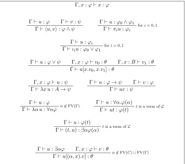
A typing judgment is a triple of the form Γ ` u : ϕ, and we use it to mean that there exists a derivation using the typing rules from Figure 2.4 with Γ`u:ϕat the root.
Definition 2.6.4(Reduction rules for MQC). We define the reduction relation
→MQC as the compatible closure of the following reduction rules:
(λx.u)t →β1 u[x:=t] (λα.u)t →β2 u[α:=t] π0hu0, u1i →π0 u0
π1hu0, u1i →π1 u1
ι0(u)[x1.t1, x2.t2] →ι0 t0[x1 :=u]
ι1(u)[x1.t1, x2.t2] →ι1 t1[x2 :=u]
(n, u)[(α, x).v] →∃ v[α:=n][x:=u], for each termn
Γ, x:ϕ`x:ϕ
Γ`u:ϕ Γ`v:ψ Γ` hu, vi:ϕ∧ψ
Γ`u:ϕ0∧ϕ1
fori= 0,1
Γ`πiu:ϕi
Γ`u:ϕi
fori= 0,1
Γ`ιiu:ϕ0∨ϕ1
Γ`u:ϕ∨ψ Γ, x:ϕ`v0 :θ Γ, x:B `v1:θ
Γ`u[x.v0, x.v1] :θ
Γ, x:ϕ`u:ψ Γ`λx u:A→ψ
Γ`u:ϕ→ψ Γ`v :ϕ Γ`uv:ψ
Γ`u:ϕ
α6∈FV(Γ)
Γ`λα u:∀αϕ
Γ`u:∀α.ϕ(α)
tis a term ofL
Γ`ut:ϕ(t)
Γ`u:ϕ(t)
tis a term ofL
Γ`(t, u) :∃αϕ(α)
Γ`u:∃αϕ Γ, x:ϕ`v:θ
α6∈FV(C)∪FV(Γ)
[image:26.595.133.508.248.579.2]Γ`u[(α, x).v] :θ
Chapter 3
Friedman’s
A
-translation
In this chapter we will present a proof of the following old theorem by Kreisel [25]:
Theorem 3.0.6. Peano Arithmetic is a conservative extension of Heyting Arithmetic over the Π02-sentences.
The proof will make use of two techniques that are central to area of classical program extraction, namely the G¨odel–Gentzen double negation translation and Friedman’s A-translation.
The theorem has the following corollary, which gives the main motivation to why we want to examine the computational content of classical proofs:
Corollary 3.0.7. A recursive function is provably total in Peano Arithmetic if and only if it is provably total in Heyting Arithmetic.
This tells us, that any classical proof of totality of a recursive function can be converted to an intuitionistic proof, and therefore the classical proof must be constructive, and have computational content in some sense.
3.1
The arithmetics
PA
and
HA
We formalize arithmetic as natural deduction systems. Firstly, we have to fix the signature of the language. Notice that we assume to have the concept of primitive recursive relations defined in our meta-language.
Definition 3.1.1 (Signature of arithmetic). Let
S ={0,S,=} ∪ {P |P is a primitive recursive relation}
where 0 is a nullary function symbol, S is a unary function symbol, = is a binary relation symbol, and P is ann-ary relation symbol, if P is ann-ary primitive recursive relation.
Then the language L=LS consists of all formulas of arithmetic. We will
use this language for iFOL and cFOL.
Notation 3.1.2. We will write Γ`I ϕif Γ`ϕin iFOL, and Γ`C ϕ if Γ`ϕin cFOL.
Definition 3.1.3(The Peano axioms). Let Ω be the (countable) set of formulas consisting of the universal closures of the following formulas.
Axioms for equality: (refl): α=α
(trans): α=β∧β=γ →α=γ
(congP): αi=α0i →(P(α1, . . . , αi, . . . , αn) =P(α1, . . . , αi0, . . . , αn)) for everyn-aryP and 1≤i≤n
(congS) α=β →Sα=Sβ Axioms for successor:
(succ1): ¬(Sα=0)
(succ2): Sα=Sβ →α=β
Induction axiom schema:
(ind): ϕ(0)∧ ∀α.(ϕ(α)→ϕ(Sα))→ ∀α.ϕ(α) for every formulaϕ(α)
Defining axioms: (succP): P(α,Sα)
(constP): P(α1, . . . , αn,Sm0) (projP): P(α1, . . . , αi, . . . , αn, αi)
(compP): R1(α1, . . . , αn, β1)∧ · · · ∧Rm(α1, . . . , αn, βm)
∧Q(β1, . . . , βm, γ)→P(α1, . . . , αn, γ) (recP): (Q(α1, . . . , αn, β)→P(0, α1, . . . , αn, β))
∧(P(γ, α1, . . . , αn, δ)∧R(δ, β, α1, . . . , αn, ε)
→P(Sγ, α1, . . . , αn, ε)) These are the Peano axioms.
Definition 3.1.4(Peano arithmetic and Heyting arithmetic). We say that a formulaϕ is derivable in Peano arithmetic, and write `PAϕ, if there is a finite
subset Γ⊂ωΩ of the Peano axioms such that Γ`C ϕ. Similarly, we say that ϕis derivable in Heyting arithmetic,`HA, if Γ`I ϕfor some Γ⊂ωΩ.
3.2
Double-negation translation
3.2. DOUBLE-NEGATION TRANSLATION 21
Definition 3.2.1 (Double-negation translation). Letϕbe a formula. Define the double-negation translation ϕ− ofϕas follows:
⊥−:=⊥
P−:=¬¬P, whereP 6=⊥is atomic
(ϕ∨ψ)−:=¬¬(ϕ−∨ψ−)
(ϕ∧ψ)−:=ϕ−∧ψ−
(ϕ→ψ)−:=ϕ−→ψ−
(∀α.ϕ)−:=∀α.ϕ− (∃α.ϕ)−:=¬¬∃α.ϕ−
Soϕ−is the result of double-negating all atomic, disjunctive and existential subformulas of ϕ.
Lemma 3.2.2 (Properties of double-negation translation). Letϕbe a formula, Γ a set of formulas, and Γ−={ψ− | ψ∈Γ}.
1. `C ϕ↔ϕ−,
2. ¬¬ϕ−`I ϕ−,
3. IfΓ`C ϕ, then Γ−`I ϕ− (this justifies calling it a translation).
Proof. 1. We need to show that ϕ `C ϕ− and ϕ− `C ϕ for any formula ϕ. This is done by induction on the complexity ofϕ, and we only have to consider the atomic, disjunctive, and existential cases. We show the atomic case, the rest are similar. For P `C ¬¬P we have the derivation
¬Px P
⊥ x
¬¬P
and for the case ¬¬P `C P we have
P∨ ¬P Px
¬¬P ¬Px
⊥
P x P
2. This is also an easy induction. We show just the atomic case, where we need¬¬¬¬ϕ`I ¬¬ϕ:
¬¬¬¬P
¬¬Py ¬Px
⊥ y
¬¬¬P
⊥ x
3. We show this by induction on the depth of the derivation Γ`C ϕ. Most of the rules are trivial, those are the rules that iFOL and cFOL have in common. See for example implication elimination:
Γ, ϕ`C ψ Γ`C ϕ→ψ
becomes Γ
−, ϕ−`
I ψ− Γ−`I ϕ−→ψ−
So we have only the excluded middle rule left. We will only have to show that `I ¬¬(ϕ∨ ¬ϕ) for any formula ϕ, it will then follow that Γ`I ¬¬(ϕ−∨ ¬ϕ−). We show this with the following derivation:
¬(ϕ∨ ¬ϕ)x
¬(ϕ∨ ¬ϕ)x
ϕy ϕ∨ ¬ϕ
⊥ y
¬ϕ ϕ∨ ¬ϕ
⊥ x
¬¬(ϕ∨ ¬ϕ)
Observation 3.2.3. In general not ϕ`I ϕ−.
This can be shown with a counter-example. One such is ¬∀α.P(α) 6`I ¬∀α.¬¬P(α), which can be shown using Kripke semantics.
3.3
A
-translation
TheA-translation was introduced by H. Friedman in [14] to give a simple proof of Kreisel’s theorem. TheA in the name stems from the name Friedman used for the arbitrary formula that is inserted via the translation.
Definition 3.3.1 (A-translation). Let ϕ and A be formulas such that no bound variable of ϕ is free in A. We define the A-translation ϕA of ϕ as follows:
⊥A:=A
PA:=P ∨A, where P 6=⊥is atomic
(ϕ∧ψ)A:=ϕA∧ψA
(ϕ∨ψ)A:=ϕA∨ψA
(ϕ→ψ)A:=ϕA→ψA
(∀α.ϕ)A:=∀α.ϕA
3.3. A-TRANSLATION 23
SoϕAis the result of substituting all atomic subformulas P with P ∨A, and replacing any ⊥with A. Note that (¬P)A=P ∨A→A.
Lemma 3.3.2 (Properties of the A-translation). Let ϕ be a formula, Γ a set of formulas and A a formula such that ϕA and ΓA are defined, where ΓA={ψA | ψ∈Γ}.
1. `C ϕA↔ϕ∨A
2. A`I ϕA
3. IfΓ`I ϕ, then ΓA`I ϕA
4. In general notϕ`I ϕA
Proof. 1. We have to show that ϕA `C ϕ∨A and ϕ∨A `C ϕA. This is easily done by induction on the complexity of ϕ. We illustrate by showing one case, that of (ϕ∧ψ)∨A`C ϕA∧ψA:
(ϕ∧ψ)∨A
ϕ∧ψx ϕ ϕ∨A
IH ϕA
ϕ∧ψx ψ ψ∨A
IH ψA
ϕA∧ψA
Ax ϕ∨A
IH ϕA
Ax ψ∨A
IH ψA
ϕA∧ψA
x
ϕA∧ψA
2. This is a straight-forward induction on the complexity of ϕ.
3. This is done by induction on the depth of the derivation of Γ`I ϕ. For the ex falso quodlibet rule, the induction hypothesis is that ΓA`IA, but from 2 we haveA`I ϕA, this together gives us ΓA`IϕA. As for the rest of the rules, they are quite simple. Here is the implication introduction case:
Γ, ϕ`ψ
Γ`ϕ→ψ becomes
IH ΓA, ϕA`ψA ΓA`ϕA→ψA
The rest of the rules without quantifiers are similarly obvious. For the quantifier rules, we have to take care of variable bindings. Here existential introduction:
Γ`ϕ[α:=t]
Γ` ∃α.ϕ becomes
IH ΓA`ϕA[α:=t]
∃I ΓA` ∃α.ϕA
Observation 3.3.3. In general not ϕ`I ϕA. A counter-example for this is ¬¬A6`I(¬¬A)A.
3.4
The proof
We know from Observation 3.2.3 and Observation 3.3.3 that it does not always hold thatϕ`I ϕ− orϕ`I ϕA. But in some cases it does hold, and these are the cases where theA-translation proof method is applicable. In our case, this isHA. We first observe some easy cases:
Observation 3.4.1. If ϕ is on one of the forms
• P,
• P∧Q,
• P1∧ · · · ∧Pm →Q, or
• (P1 →P2)∧(Q1∧Q2→Q3),
where P, P1, . . . , Pm, Q, Q1, Q2, Q3 are atomic formulas, then ϕ `I ϕ− and
ϕ`I ϕA.
This leads us to the following interesting lemma:
Lemma 3.4.2. Let ϕ be a Peano axiom. Then`HA ϕ− and `HA ϕA.
Proof. Every axiom, except the induction axiom, is on one of the shapes from Observation 3.4.1. So we only need to check the induction axiom: Letϕbe an instance of the induction axiom:
ϕ=ψ(0)∧ ∀α(ψ(α)→ψ(S(α)))→ ∀α.ψ(α),
for some formulaψ(α). Now:
ϕ−=ψ−(0)∧ ∀α(ψ−(α)→ψ−(S(α)))→ ∀α.ψ−(α),
ϕA=ψA(0)∧ ∀α(ψA(α)→ψA(S(α)))→ ∀α.ψA(α),
which are themselves axioms of HA.
Corollary 3.4.3. Let ϕ and A be formulas. 1. If `PAϕ, then `HAϕ−;
2. If `HAϕ and ϕA is defined, then `HA ϕA.
Proof. 1. Let Γ be the axioms used in the derivation`PAϕ.
3.4. THE PROOF 25
2. Let Γ be the axioms used in the derivation`HA ϕ.
Γ`I ϕ =⇒ ΓA`I ϕA =⇒ `HA ϕA.
Definition 3.4.4 (Π02-, Σ01-formulas). A Σ01-formula is of the form
∃α1· · · ∃αn.ϕ(α1, . . . , αn), whereϕis quantifier-free. If ψis a Σ01-formula, then
∀α1· · · ∀αn.ϕ(α1, . . . , αn), is called a Π02-formula.
We will use the following fact to simplify the Σ01-formulas:
Lemma 3.4.5. For any quantifier-free formula ϕ(α1, . . . , αn), there is a prim-itive recursive relation P(α1, . . . , αn) such that
`HA ϕ(α1, . . . , αn)↔P(α1, . . . , αn).
Thus, whenever we talk about a Σ01-formula, we only need to consider the ones of the form∃α.P(α).
Lemma 3.4.6. If ϕis a Σ01-formula, then `I ϕA↔ϕ∨A. Proof. Firstly, one can check that
∃α.(ϕ∨ψ)↔ ∃α.ϕ∨ψ,
whenever α6∈FV(ψ). Let now ∃α.P(α) be a Σ01-formula. Then (∃α.P(α))A=∃α.(P(α)∨A),
and so
`I(∃α.P(α))A↔ ∃αP(α)∨A.
Proof of Theorem 3.0.6
We need to show that `PAϕ if and only if `HA ϕfor any Π02-sentence ϕ. It is sufficient to show that `PAϕ if and only if`HA ϕ for any Σ01-formula, for
whenever we have a Σ01-formula ϕ(α1, . . . , αn) for which `HA ϕ(α1, . . . , αn) holds, we can apply n universal quantifier introduction rules to close it, in order to get a proof of the Π0
Let ∃α.P(α) be a given Σ0
1-formula, and setA:=∃α.P(α). Assume that
`PA A. We first do a double-negation translation, and get `HA ¬¬A. By A-translation, we get`HA (¬¬A)A. But
(¬¬A)A= (AA→A)→A,
and since `HAAA↔A∨A↔A, and so `HAAA→A, we get
`HA (¬¬A)A↔A.
Chapter 4
Control operators
Theλ-calculus has for a long time been seen as a natural basis for programming languages, and has thus been used as a meta-language to describe features in programming languages at least since Landin used it to study the features of Algol 60 [27]. Since theλ-calculus is purely functional it cannot be used
to describe the jumps and labels of Algol 60, and therefore Landin had
to extend the calculus with the non-functional operator J, an example of a control operator—an operator that behaves in a non-local way in order to change the control flow of the program execution. Control operators have since been introduced to functional programming languages. The Scheme dialects, e.g., have control operators equal in power to J, namely catch andthrow [38] and call-with-current-continuation (call/cc) [35]. According to Talcott, the advantage of using control operators is that they “provide a way of pruning unnecessary computation and allow certain computations to be expressed by more compact and conceptually manageable programs.” [40].
It was later discovered by Griffin [20] that adding control operators to typed λ-calculi corresponds, via the Curry–Howard correspondence, to adding classical reasoning to the logic. He did this by observing that Felleisen’s extension of theλ-calculus with control operators [13] could be typed in such a way that the types of the control operators corresponded toex falso quodlibet and double negation elimination.
In this chapter we will first introduce the systemλµ by Parigot [30] which is an extension to simply typed λ-calculus which by means of adding the µ-operator makes it possible to define call/cc andcatch-throw, and with which it is possible to define terms with types that are not otherwise allowed in intuitionistic systems, e.g. Peirce’s law. Secondly, in order to get closer to a “real” programming language, we will introduce theλµT-calculus by Geuvers,
Krebbers and McKinna [16] which is an extension of the λµ-calculus adding the natural numbers as a primitive datatype with a primitive recursor in the style of G¨odel’s system T.
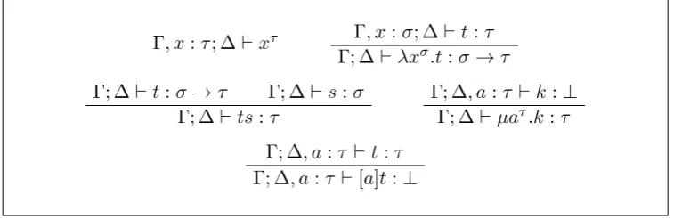
Γ, x:τ; ∆`xτ Γ, x:σ; ∆`t:τ Γ; ∆`λxσ.t:σ →τ
Γ; ∆`t:σ→τ Γ; ∆`s:σ Γ; ∆`ts:τ
Γ; ∆, a:τ `k:⊥
Γ; ∆`µaτ.k:τ
[image:36.595.131.510.127.250.2]Γ; ∆, a:τ `t:τ Γ; ∆, a:τ `[a]t:⊥
Figure 4.1: Typing rules for λµ
4.1
The system
λµ
In 1992 M. Parigot [30] introduced the λµ-calculus as a way of extending the Curry–Howard correspondence to classical proofs, by way of adding the control operator µto the simply typed lambda calculus. Together with the control operator we also introduce a special kind of variables, theµ-variablesor addresses. Therefore, the environments inλµ will be bipartite; an environment will consist of a set Γ of λ-variables together with types as usual, and a set ∆ ofµ-variables together with types.
Definition 4.1.1 (Terms of λµ). The terms of λµ are defined inductively over an infinite set ofλ-variables (x, y, z, . . .) and an infinite set ofµ-variables (a, b, c, . . .) as follows
t, s::=x |λxτ.t|ts |µaτ.k
k::= [a]t
Here,τ ranges over simple types as defined in Definition 2.4.1.
Definition 4.1.2 (Free variables). We let FV(t) denote the set of free λ -variables int, while FCV(t) denotes the set of freeµ-variables.
Definition 4.1.3 (Typing judgments inλµ). The types ofλµ are the same as those inλ→ (Definition 2.4.1), with an extra atomic type⊥(read bottom).
A typing judgment Γ; ∆`t:ρ is derivable in λµ if there is a derivation tree that uses the rules of Figure 4.1 with Γ; ∆`t:ρ as the conclusion.
Notice that the first three rules in Figure 4.1 are the same as the rules of λ→ (Figure 2.2). The two new rules are known as, respectively,activate and
passivate.
Example 4.1.4. Inλµ we can inhabit the type of the non-intuitionisticPeirce’s law ((p→q)→p)→p. We get the term
4.1. THE SYSTEM λµ 29
x: (p→q)→p
z:p [a]z:⊥
µbq.[a]z:q λzpµbq.[a]z:p→q x(λzpµbq.[a]z) :p
[a]x(λzpµbq.[a]z) :⊥
µap.[a]x(λzpµbq.[a]z) :p
λx(p→q)→pµap.[a]x(λzpµbq.[a]z) : ((p→q)→p)→p
Theorem 4.1.5. The strength of λµ is exactly minimal classical propositional logic. I.e.,
Γ`ϕin minimal classical logic
⇐⇒
there is some term t in λµ such that Γ;∅ `t:ϕ.
A proof of this can be found in [24].
Reduction in λµ
In order to define the reduction rules we need to introduce a new notion of substitution, namely structural substitution.
Definition 4.1.6 (Call-by-name contexts). Acall-by-name evaluation context is defined as
E ::=|Et,
wheretranges over terms.
Definition 4.1.7(Structural substitution). Lettbe aλµ-term, and leta, bbe µ-variables and E a call-by-name evaluation context. We define the structural substitution t[a:=bE] of band E foraby induction as follows:
x[a:=bE] :=x
(λx.t)[a:=bE] :=λx.t[a:=bE]
(ts)[a:=bE] :=t[a:=bE]s[a:=bE]
(µa.k)[a:=bE] :=µa.k
(µc.k)[a:=bE] :=µc.k[a:=bE] ifc6=a
Definition 4.1.8(Reduction). We define the reduction relation→ on λµas the compatible closure of the following rules:
(λx.t)s →β t[x:=s]
(µa.k)t →µR µa.k[a:=a(t)] µa.[a]t →µη t ifa6∈FCV(t) [a]µb.k →µι k[b:=a]
Definition 4.1.9 (Catch and throw). We define the terms catcha t and throwa tas follows:
catcha t:=µa.[a]t
throwa t:=µb.[a]t whereb6∈FCV([a]t)
Lemma 4.1.10. The terms catch and throw behaves as follows, where E is a call-by-name context:
1. E[throwa t]throwa t,
2. catcha (throwa t)catcha t
3. catcha tt if a6∈FCV(t)
4. throwb (throwa t)throwa t
Proof. For the first reduction, do an induction on the structure ofE. The rest follows directly from the definitions and the reduction rules.
The λµ-calculus satisfies the main meta-theoretical theorems:
Theorem 4.1.11. λµ is confluent.
Proof. A proof can be found in [24].
Theorem 4.1.12. λµ satisfies subject reduction.
Proof. A proof can be found in [24].
Theorem 4.1.13. λµ is strongly normalizing.
4.2. THE SYSTEM λµT 31
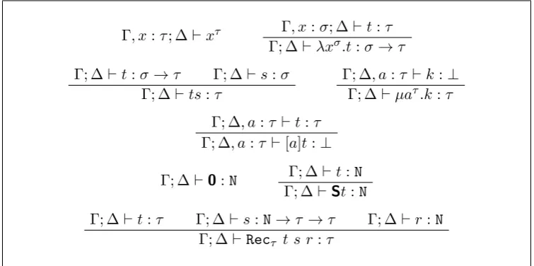
Γ, x:τ; ∆`xτ Γ, x:σ; ∆`t:τ Γ; ∆`λxσ.t:σ→τ
Γ; ∆`t:σ →τ Γ; ∆`s:σ Γ; ∆`ts:τ
Γ; ∆, a:τ `k:⊥
Γ; ∆`µaτ.k:τ
Γ; ∆, a:τ `t:τ Γ; ∆, a:τ `[a]t:⊥
Γ; ∆`0:N Γ; ∆`t:N Γ; ∆`St:N
[image:39.595.86.464.126.314.2]Γ; ∆`t:τ Γ; ∆`s:N→τ →τ Γ; ∆`r:N Γ; ∆`Recτ t s r:τ
Figure 4.2: Typing rules forλµT
4.2
The system
λµ
TTheλµT-calculus arises from the λµ-calculus in the same way that the λT -calculus arises from the λ→-calculus, namely by “hard-coding” the natural
numbers into the system by adding an atomic type N, primitive terms 0:N and S:N→N, and a recursor Rec.
Definition 4.2.1 (Terms of λµT). The terms of λµT are defined inductively
over an infinite set of λ-variables (x, y, z, . . .) and an infinite set ofµ-variables (a, b, c, . . .) as follows:
t, s, r:=x |λxτ.t |ts|µaτ.k |0|St|Recτ t s r
k:= [a]t
Here, τ ranges overλT-types, as defined in Definition 2.5.1.
Definition 4.2.2 (Free variables). As inλµ, we let FV(t) and FCV(t) denote the sets of free λ-variables andµ-variables, respectively.
We define substitutiont[x:=s] in the obvious way, such that it is capture avoiding for both λ- andµ-variables.
Definition 4.2.3 (Typing judgments inλµT). A typing judgment Γ; ∆`t:ρ isderivable in λµT if there is a derivation tree that uses the rules of Figure 4.2 with Γ; ∆`t:ρas the conclusion, and similarly, a typing judgment Γ; ∆`k:⊥
is derivable in λµT in case it is the conclusion of such a derivation tree.
Proof. By easy induction on the depth of the derivation.
When we work withnumerals, we will abbreviate them as n:=Sn0. In order to define reduction in λµT we will first need the concepts of contexts and structural substitution.
Definition 4.2.5(Contexts). We define theλµT-contexts as follows: E ::=|Et |SE |Rect s E,
Such a context issingular if the depth of the is exactly one, i.e.:
Es ::=t|S|Rec t s.
Definition 4.2.6 (Context substitution, composition). Given a context E and a termt, we define E[s] as follows:
[s] :=s (Et)[s] :=E[s]t
(SE)[s] :=SE[s]
(Rect s E)[s] :=Rect s E[s]
Given two contexts E and F, we define their composition EF thus:
F :=F (Et)F := (EF)t
(SE)F :=S(EF)
(Rec t s E)F :=Rect s(EF)
Definition 4.2.7(Structural substitution). We define the structural substi-tution t[a := bE] of a µ-variable b and a context E for a µ-variable a as
follows:
x[a:=bE] :=x
(λx.t)[a:=bE] :=λx.t[a:=bE]
(ts)[a:=bE] :=t[a:=bE]s[a:=bE]
0[a:=bE] :=0
(St)[a:=bE] :=S(t[a:=bE])
(Rect s r)[a:=bE] :=Rec(t[a:=bE]) (s[a:=bE]) (r[a:=bE])
(µc.k)[a:=bE] :=µc.k[a:=bE]
([a]t)[a:=bE] := [b]E[t[a:=bE]]
([c]t)[a:=bE] := [c]t[a:=bE] ifc6=a
4.2. THE SYSTEM λµT 33
Definition 4.2.8 (Reduction rules ofλµT). We define the reduction relation
→ as the compatible closure of the following rules:
(λx.t)s →β t[x:=s]
S(µa.k) →µS µa.k[a:=a (S)] (µa.k)t →µR µa.k[a:=a (t)]
µa.[a]t →µη t ifa6∈FCV(t) [a]µb.k →µi k[b:=a] Rect s 0 →0 t
Rect s (Sn) →S s n(Rect s n)
Rect s (µa.k) →µN µa.k[a:=a (Rect s )]
TheλµT-calculus fulfills the following important meta-theorems, proofs for all of which can be found in [16].
Theorem 4.2.9 (Subject reduction). The λµT-calculus satisfies subject re-duction, i.e., if Γ; ∆`t:τ andt→t0, then Γ; ∆`t0 :τ.
Theorem 4.2.10 (Confluence). The reduction relation → is confluent, i.e., if t1 t2 andt1 t3, then there is a term t4 such thatt2 t4 andt3 t4.
t1
t2 t3
t4
Theorem 4.2.11 (Strong normalization). λµT is strongly normalizing: If Γ; ∆`t:σ, then there is no infinite reduction chain
Chapter 5
Arithmetic with exceptions:
HA
+
EM
1
In this chapter we present Aschieri and Berardi’s system HA+EM1 [6], and
show its strong normalization, using a new proof method by Aschieri [3]. The system is an extension of Heyting arithmetic with a restricted version of the law of the excluded middle, EM1, which allows us to use in our proofs all
disjunctions of the form ∀α.P(α)∨ ∃α.¬P(α), whereP is an atomic formula. There are multiple reasons for choosing the restricted version EM1. In
contrast to the full EM, the truth of EM1 can be computed in the limit, in the
sense of Gold [19]. Every time an instance P(n) of the hypothesis ∀α.P(n) is used, it can effectively be checked whether this instance is true or not. If it is not, then we are immediately provided with a witness for the truth of
∃α.¬P(α).
Furthermore, many important classical theorems of mathematics can be proved with only EM1 [1, 10].
5.1
Post rules
Since we will describe a mathematical theory we need an atomic language and non-logical axioms. The computations that we are interested in are not the ones that happen at the atomic level, so therefore we will not bother with actually describing it. Instead, we will use Post rules as in [34] to cover up the computations happening at the atomic level, in order to simplify the low-level reasoning.
Definition 5.1.1. APost rule is an inference rule of the form
P1 P2 · · · Pn
Q
where P1,P2, . . . ,Pn,Q are atomic formulas, such that for every substitution
σ = [α1 := n1, α2 := n2, . . . , αk := nk], P1σ ≡ · · · ≡ Pnσ ≡ True implies Qσ≡True.
Since we work in arithmetic, we will assume there to be Post rules for every purely universal arithmetical fact that holds in the standard model ofPA, i.e. facts of the form
∀~x(P1(~x)∧ · · · ∧Pn(~x)→Q(~x)),
wherePi, Qare atomic formulas. This includes all the Peano axioms except for the induction axiom scheme. We have, for example, the axioms of equality:
(refl)
eq(t, t) eq(t1, t2) eq(t2, t3) (trans) eq(t1, t3)
eq(t1, t2) P[α:=t1]
(congP)
P[α:=t2]
And the Peano axioms for the successor:
eq(St1,St2)
(succ1)
eq(t1, t2)
eq(0,St)
(succ2)
⊥
where⊥ is the false relation, for which we have the ex falso Post rule
⊥
P
This rule is what makes our system intuitionistic, by making the ex falso rule admissible to the system.
Also, we have Post rules for all defining axioms of each primitive recursive relation, e.g.
add(t,0, t) add(add(tt1, t2, t3)
1,St2,St3)
mult(t,0,0) mult(t1, tmult(2, t3)t add(t1, t3, t4)
1,St2, t4)
A trick that we will make use of below is to weaken a Post rule. Given a rule
P1 P2 · · · Pn
Q
it can be useful to add an irrelevant premise, such that it becomes
P1 P2 · · · Pn S
Q
5.2. HA 37
5.2
HA
We can now definasdfe the first-order system of Heyting arithmetic,HA, which will be used as the basis on which we can add classical reasoning.
To start with, we formally fix the language.
Definition 5.2.1 (Variables). We have two different types of variables:
• Numerical variables,α, β, γ, representing natural numbers.
• Proof term variables, x, y, z, which correspond to the usual lambda calculus variables.
Definition 5.2.2 (Formulas of HA). We define the languageL of HA. 1. The terms in L:
t, r::=0 |St|α
whereα ranges over numerical variables. Anumeral is a closed term, i.e., a term of the formS· · ·S0.
2. There is an atomic formula P(t1, . . . , tn) for each primitive recursive relation P ⊆ Nn. If P(~t) is a closed atomic formula, i.e., all t
i are numerals, then we can write either P(~t)≡True or P(~t)≡Falseif~t∈P or~t6∈P, respectively.
3. The formulas, ϕ, ψ, θ, are built from atomic formulas by the connectives
∨,∧,→,∀,∃ as usual, with quantifiers ranging over numeric variables α, β, γ, . . ..
The negation of an atomic formula P⊥(~t) is defined as the atomic formula representing the complementing primitive recursive relation Nn\P, while the negation of a non-atomic formula ¬ϕ is defined in the usual way as ϕ→ ⊥, where⊥is the atom representing the empty relation. Notice that negation of atoms is an involution: (P⊥)⊥≡P.
Definition 5.2.3 (Free variables). Given a formulaϕ, the set FV(ϕ) is defined as the set of numerical variables occurring in ϕ that are not bound by any quantifiers.
Definition 5.2.4 (Capture avoiding substitution in formulas ofHA). Lett, r be terms of L andα a numerical variable. We firstly define r[α:=t], r with t substituted for α, recursively onr as follows:
• 0[α:=t] :=0,
• (Sr)[α:=t] :=Sr[α:=t],
• β[α:=t] :=β.
Let now ϕ be any formula. We define ϕwith t substituted forα,ϕ[α:=t], recursively onϕas follows:
• P(t1, . . . , tn)[α:=t] :=P(t1[α:=t], . . . , tn[α:=t]),
• (ϕ∨ψ)[α:=t] :=ϕ[α:=t]∨ψ[α:=t],
• (ϕ∧ψ)[α:=t] :=ϕ[α:=t]∧ψ[α:=t],
• (ϕ→ψ)[α:=t] :=ϕ[α:=t]→ψ[α:=t],
• (∀α.ϕ)[α:=t] :=∀α.ϕ,
• (∀β.ϕ)[α:=t] :=∀β.ϕ[α:=t],
• (∃α.ϕ)[α:=t] :=∃α.ϕ,
• (∃β.ϕ)[α:=t] :=∃β.ϕ[α:=t].
Definition 5.2.5 (Proof terms ofHA). The untyped proof terms in HAare the following:
u, v, w := x |uv |un |λx u|λα u
| hu, vi | π0u|π1u |ι0u |ι1u
| u[x.v, y.w]|(n, u) |u[(α, x).v]
| Recu v n|ru1 · · · um
where x, y range over proof term variables andn over L-terms. The term r will be used to represent usages of Post rules.
Definition 5.2.6(Capture avoiding substitution in terms of HA). We define two notions of capture free substitution in terms ofHA: Let u, vbe terms of HA,t a term ofL,α a numerical variable andx a λ-variable. We define the notionsu[x:=v] and u[α:=t] in the standard way.
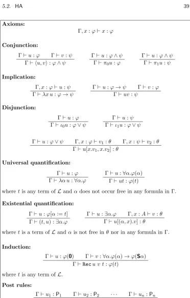
Definition 5.2.7(Typing judgments in HA). An environment, Γ, in HAis a finite set of pairs of distinctλ-variables and types. It is typically written on the form Γ =x1 :ϕ1, . . . , xn:ϕn.
A typing judgment is a triple of the form Γ ` u : ϕ, and we use it to mean that there exists a derivation using the typing rules from Figure 5.1 with Γ`u:ϕat the root.
The following lemma tells us that we can encode any quantifier-free formula into an atom, if we wish.
5.2. HA 39
Axioms:
Γ, x:ϕ`x:ϕ
Conjunction:
Γ`u:ϕ Γ`v:ψ Γ` hu, vi:ϕ∧ψ
Γ`u:ϕ∧ψ Γ`π0u:ϕ
Γ`u:ϕ∧ψ Γ`π1u:ψ
Implication:
Γ, x:ϕ`u:ψ Γ`λx u:ϕ→ψ
Γ`u:ϕ→ψ Γ`v :ϕ Γ`uv:ψ
Disjunction:
Γ`u:ϕ Γ`ι0u:ϕ∨ψ
Γ`u:ψ Γ`ι1u:ϕ∨ψ
Γ`u:ϕ∨ψ Γ, x:ϕ`v1 :θ Γ, x:ψ`v2 :θ
Γ`u[x.v1, x.v2] :θ
Universal quantification: Γ`u:ϕ Γ`λα u:∀α.ϕ
Γ`u:∀α.ϕ(α) Γ`ut:ϕ(t)
wheretis any term of Land α does not occur free in any formula in Γ.
Existential quantification: Γ`u:ϕ[α:=t] Γ`(t, u) :∃α.ϕ
Γ`u:∃α.ϕ Γ, x:A`v:θ Γ`u[(α, x).v] :θ
wheretis a term of L and α is not free inθ nor in any formula in Γ.
Induction:
Γ`u:ϕ(0) Γ`v:∀α.ϕ(α)→ϕ(Sα) Γ`Recu v t:ϕ(t)
wheretis any term of L.
Post rules:
Γ`u1 :P1 Γ`u2:P2 · · · Γ`un:Pn Γ`ru1 u2 · · · un:Q
[image:47.595.87.460.87.669.2]whereP1, . . . ,Pn,Qare atomic formulas and the rule is a Post rule in arithmetic. If there are no premises to the rule, we will write Trueinstead of r.
Proof. The proof is by induction on the complexity ofϕ. By definition, the atomic case is trivial. For ϕ∧ψ, there are primitive recursive relationsP1,P2
corresponding toϕ and ψ respectively. Define P as the primitive recursive relation that is true whenever bothP1 and P2 are true. Similarly with ∨. For
ϕ→ ψ, define P as the relation that is true when P2 is true, or when P1 is
false.
Reduction for HA
Definition 5.2.9 (Reduction rules forHA). We define the reduction relation
→HA as the compatible closure of the following reduction rules: (λx.u)t →β1 u[x:=t]
(λα.u)t →β2 u[α:=t] π0hu0, u1i →π0 u0
π1hu0, u1i →π1 u1
ι0(u)[x1.t1, x2.t2] →ι0 t0[x0 :=u]
ι1(u)[x1.t1, x2.t2] →ι1 t1[x1 :=u]
(n, u)[(α, x).v] →∃ v[α:=n][x:=u], for each numeraln
Recu v 0 →Rec1 u
Recu v (Sn) →Rec2 v n(Recu v n)
The following lemma tells us that the logic is indeed intuitionistic.
Lemma 5.2.10(Ex falso quodlibet). There exist a termefqϕ for any formula ϕsuch that
`efqϕ :⊥ →ϕ.
Proof. We show this by induction on the complexity of the formulaϕ.
• ϕ=P (atomic): Since we have the Post rule
⊥
P
for any atomic formulaP we have the following derivation:
x:⊥ `x:⊥
x:⊥ `rx:P
`λx.rx:⊥ →P
soefqP :=λx.rx.
• ϕ=ψ1∧ψ2: Letefqψ1∧ψ2 :=λxhefqψ1x,efqψ2xi, for
x:⊥ `efqψ1x:ψ1 x:⊥ `efqψ2x:ψ2
x:⊥ ` hefqψ1x,efqψ2xi:ψ1∧ψ2
5.3. HA+EM1 41
• ϕ=ψ1 →ψ2: Letefqψ1→ψ2 :=λxλyefqψ2x, for
x:⊥, y:ψ1 `efqψ2x:ψ2
x:⊥ `λyefqψ2x:ψ1 →ψ2
`λxλyefqψ2x:⊥ →ψ1 →ψ2
• ϕ=∀α ψ: Similarly, let efq∀αψ :=λxλαefqψx.
• ϕ=ψ1∨ψ2: Letefqϕ =λx ι0(efqψ1x):
x:⊥ `efqψ1x:ψ1
x:⊥ `ι0(efqψ1x) :ψ1∨ψ2
`λx ι0(efqψ1x) :⊥ →ψ1∨ψ2
• ϕ=∃α ψ: Let efq∃α ψ =λx(0,efqψ[α:=0]x):
x:⊥ `efqψ[α:=0]x:ψ[α:=0]
x:⊥ `(0,efqψ[α:=0]x) :∃α ψ
`λx(0,efqψ[α:=0]x) :⊥ → ∃α ψ
5.3
HA
+
EM
1The system HA+EM1, introduced by Aschieri, Berardi and Birolo in [6],
arises from HAby adding a limited amount of classical reasoning, namely the EM1-rule, the law of excluded middle restricted to Π01-formulas. Often, one
sees the law of excluded middle defined as a rule of the form
ϕ∨ ¬ϕ
But since this classical axiom does not contain any computational content by itself, we will instead combine it with the disjunction elimination rule to obtain an elimination rule of the form
[ϕ] .. . ψ
[¬ϕ] .. . ψ ψ
Since we will only consider the restricted EM1-rule, we can instead of ϕand
The informal computational intuition behind this proof rule is roughly the following: We start by assuming the truth of ∀α.P(α), and then each time we need the truth of an instance P(n) of the assumption, we check whether it is true or not; if it is true, then we continue, if it is not, we have found a witness for ∃α.P⊥(α) which we can then fill in in the right-hand-side of the proof. The crucial observation is then that we will only ever need a finite number of instances of∀α.P(α) to prove ϕ.
Definition 5.3.1(Variables inHA+EM1). We will operate with three different
types of variables:
• Numerical variables,α, β, γ, to represent natural numbers.
• Proof term variables,x, y, z, that act like usual lambda calculus variables.
• Hypothesis variables,a, b, c, which act as addresses to refer to uses of EM1 hypotheses.
Definition 5.3.2 (Formulas of HA+EM1). The atomic language and the
formulas ofHA+EM1 are the same as for HA, see Definition 5.2.2.
The proof terms of HA+EM1 are similar to those of HA, except we add
terms to take care ofEM1 hypotheses.
Definition 5.3.3(Proof terms of HA+EM1). The untyped proof terms are
the following:
u, v, w::=x |uv |um |λx u|λα u | hu, vi |π0u |π1u |ι0u |ι1u
|u[x.v, y.w]|(m, u) |u[(α, x).v]|ukav |H∀aα.P(α)
|Wa∃α.P⊥(α) |Recu v m |ru1. . . un
where x, y range over proof term variables,aover hypothesis variables and m overL-terms. In terms of the formukavwe assume thataonly occurs free in
uin subterms of the form H∀aα.P(α), and inv in subterms of the form W∃α.P
⊥(α)
a .
Ifroccurs as a subterm without any accompanyingu’s, we will instead write True.
Definition 5.3.4(Capture avoiding substitution, witness substitution). We define the substitutions u[α := t] and u[x := v] like in HA. We also define witness substitution: Let u be a term and n a numeral. Define u[a := n]
as the term obtained from replacing each subterm W∃α.P
⊥(α)
5.3. HA+EM1 43
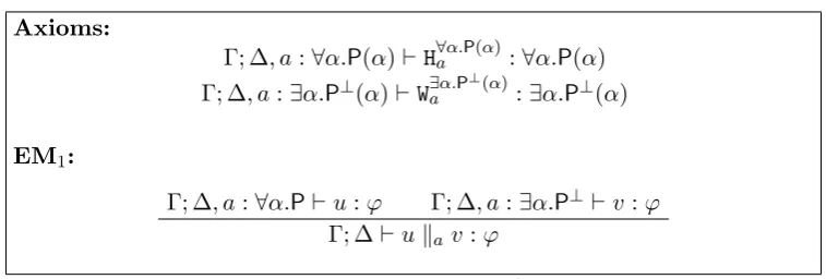
Axioms:
Γ; ∆, a:∀α.P(α)`Ha∀α.P(α):∀α.P(α) Γ; ∆, a:∃α.P⊥(α)`W∃α.P
⊥(α)
a :∃α.P⊥(α)
EM1:
[image:51.595.85.464.121.249.2]Γ; ∆, a:∀α.P`u:ϕ Γ; ∆, a:∃α.P⊥`v:ϕ Γ; ∆`ukav:ϕ
Figure 5.2: Typing rules for EM1
Definition 5.3.5(Typing judgments ofHA+EM1). EnvironmentsinHA+EM1
are bipartite: They consist of a set Γ similar to the environments from HA consisting of λ-variables and types, and then a set ∆ with pairs of hypothesis variables and formulas. We write Γ; ∆ where Γ = x1 :ϕ1, . . . , xn :ϕn and ∆ =a1 :ψ1, . . . , am:ψm.
We write the typing judgment Γ; ∆`u:ϕwhere Γ; ∆ is an environment, u a HA+EM1-term and ϕa formula, to mean that there is a derivation using
the typing rules from Figure 5.1 (where the content of ∆ is irrelevant) and from Figure 5.2.
Definition 5.3.6 (Free variables). We define FV(u) to be the set of free λ-variables inu, FNV(u) to be the set of free numeric variables and FCV(u) to be the set of free hypothesis-variables inu, where a hypothesis variableais said to be free if there is a subterm of the form H∀aα.P(α)or W
∃α.P⊥(α)
a not in the scope of ka.
The free numeric variables ofH∀aα.P(α) andW∃α.P
⊥(α)
Reduction for HA+EM1
Definition 5.3.7(Reduction rules for HA+EM1). We define the reduction
relation→HA+EM1 as the compatible closure of the following reduction rules: (λx.u)t →β1 u[x:=t]
(λα.u)t →β2 u[α:=t] π0hu0, u1i →π0 u0
π1hu0, u1i →π1 u1
(ι0u)[x0.v0, x1.v1] →ι0 v0[x0 :=u]
(ι1u)[x0.v0, x1.v1] →ι1 v1[x1 :=u]
(n, u)[(α, x).v] →∃ v[α :=n][x:=u], for each numeraln
Rec u v0 →Rec1 u
Recu v (Sn) →Rec2 v n(Recu v n) (ukav)w →perm1 uwkavw
πi(ukav) →perm2 πiukaπiv
(ukav)[x.w1, y.w2] →perm3 u[x.w1, y.w2]kav[x.w1, y.w2]
(ukav)[(α, x).w] →perm4 u[(α, x).w]kav[(α, x).w]
H∀aα.P(α)n →EM11 r, ifP(n) =True
ukav →EM12 u, ifadoes not occur free inu
ukav →EM13 v, ifadoes not occur free inv
ukav →EM14 v[a:=n], ifH
∀α.P(α)
a noccurs in u and P(n) =False
Definition 5.3.8(Normal forms). Define NFto be the set of all proof terms in normal form, andSNto be the set of strongly normalizing proof terms. We say that a term is in Post normal form if it is recursively built up with rand H∀aα.P(α) n, wheren is a numeral, as follows:
p::=rp· · ·p |H∀aα.P(α) n.
A term in Post normal form represents a derivation that only consists of Post rules and instances of a universal hypothesis. We usePNF to refer to the set of terms in Post normal form.
Example 5.3.9. We will see how we can perform proofs by contradiction in this system. Classically, we are used to be able to reason like this:
Γ,∀αP⊥` ⊥
Γ` ∃αP
In the current system, we can do this with the following derivation:
Γ, a:∀αP⊥`efq
∃αP:⊥ → ∃αP Γ, a:∀αP⊥`u:⊥
Γ, a:∀αP⊥`efq∃αPu:∃αP Γ, a:∃αP`W∃aαP:∃αP