Estimation in a linear multivariate measurement error model with a change point in the data

Estimation in a linear multivariate measurement

error model with a change point in the data

Alexander Kukush

, Ivan Markovsky

, Sabine Van Huffel

Abstract

A linear multivariate measurement error model AX=B is considered. The errors inhA B i

are row-wise finite dependent, and within each row, the errors may be correlated. Some of the columns may be observed without errors, and in addition the error covariance matrix may differ from row to row. The columns of the error matrix are united into two uncor-related blocks, and in each block, the total covariance structure is supposed to be known up to a corresponding scalar factor. Moreover the row data are clustered into two groups, according to the behavior of the rows of true A matrix. The change point is unknown and estimated in the paper. After that, based on the method of corrected objective function, strongly consistent estimators of the scalar factors and X are constructed, as the numbers of rows in the clusters tend to infinity. Since Toeplitz/Hankel structure is allowed, the results are applicable to system identification, with a change point in the input data.

Key words: Linear errors-in-variables model; Corrected objective function; Clustering; Dynamic errors-in-variables model; Consistent estimator.

1 Introduction

We deal with a multivariate multiple errors-in-variables (EIV) model. Our assump-tions are rather general and comprise both the element-wise weighted total least squares problem, see Kukush and van Huffel (2004), and the structured total least squares problem, see Kukush et al. (2005b). A key condition in these papers is that

1 _{K.U.Leuven, ESAT-SCD, Kasteelpark Arenberg 10, B-3001 Leuven-Heverlee, Belgium,}

[email protected]

2 _{School of Electronics and Computer Science, University of Southampton, SO17 1BJ,}

UK,[email protected]

3 _{Kiev National Taras Shevchenko University, Vladimirskaya st. 64, 01033, Kiev, Ukraine,}

[email protected]

the noise covariance structure is known up to a scaling factor. One can argue that such a knowledge is again respective in practice.

The EIV models with two or more unknown noise parameters, however, are non-identifiable by second order methods. This problem of non-identifiability is well known in the context of the Frisch scheme, see Frisch (1934) and De Moor (1988). A similar negative result for dynamical systems is first proven in Anderson (1985).

Various additional assumptions can be imposed in order to make the EIV estima-tion problem with unknown noise covariance structure identifiable. An overview of methods for EIV system identification is given in Söderström et al. (2002).

In this paper, we assume that the errors matrix is partitioned into two uncorre-lated blocks, and in each block, the total covariance structure is known up to a corresponding scalar factor. The condition about the two unknown scalar factors is common, e.g., such situation arises in dynamic case where the input and output matrices A and B are stochastically independent and their covariance structures are known up to two scalars,λAandλB, say. Similar problems arise in static cases, see

Cirrincione et al. (2001). Zheng (1998) proposed bias-estimated least-squares esti-mated algorithms for such dynamic problems. See overview of different approaches in Agüero and Goodwin (2006). Zheng (1998) assumed the true input process to be stationary with rational spectral density, while the input and output errors to be white noises. In the present paper we allow the true input and measurement errors to have similar covariance structure, which causes non-identifiability of the system.

We show that the new assumption enables to derive the consistent parameter and noise variance estimates. Namely, we assume that the true row data are clustered into two groups. This corresponds to a change point in case of a dynamical EIV model. The first attempt to use clustering in a linear measurement error model with unknown noise variances was made by Wald (1940), where the scalar case is treated. The idea used in the paper was to cluster the data into two groups and draw a straight line through the means of the two groups. The clustering criterion is that the means are asymptotically separated from each other. Only the first em-pirical moment is used in the construction of the estimator for the slope and the intercept.

We further develop and extend the approach of Wald (1940). Our clustering as-sumption is based on the second moment of the rows of true matrix. In the scalar case, it is possible that the means in the groups are close to each other but our clus-tering condition still holds. We allow groups with the same mean but with different dispersions. In a scalar model considered by Wald (1940), our resulting estimator is different from Wald’s estimator since we utilize the second empirical moment also.

The proposed estimation procedure consists of three steps: 1) cluster the data into two groups, 2) estimate the noise variancesλA andλB, and 3) estimate the

the first step is rather simple and based on the second empirical moment. The op-timization problem in the second step is, in general, nonconvex and nonsmooth. In our simulation examples, we apply general optimization methods for its solution, e.g., the simplex method, see Nelder and Mead (1965). The third step involves an eigenvalue decomposition of a symmetric matrix, so it is computationally inexpen-sive.

The assumptions that the data can be clustered means that the true input its changes character, while the noise properties remain the same. This assumption can be viewed equivalently as having a set of data records from experiments with differ-ent true inputs. Such an assumption is certainly restrictive. The proposed method is not applicable to the problems where the inputs are stationary, which is a typical assumption in most of the earlier works on EIV system identification. The situa-tion is similar to Wald’s estimator in the present case. Madansky (1959) noted that when clusters are given a priori, Wald’s method is an instrumental variables method for estimating the slope, but this is not the case when the clusters are chosen from the data. Indeed, Pakes (1982) shows that Wald’s estimator is inconsistent when there is no change point in the data and clusters are chosen by the data in the way recommended by Wald.

We mention here two papers which are closely related to the present work. In the technical report Kukush et al. (2005a), a similar approach is used for two inputs two outputs systems, which means that the change point in the input data is known. In Markovsky et al. (2006) another estimator is proposed in the presence of two clusters. That estimator is easier to compute but its asymptotic properties are un-clear.

We use the following notations. kAk is the Frobenius norm of the matrix A. Ip

denotes a unit matrix of size p. For a symmetric matrix C,µ1(C)≤. . .≤µp(C)are

the p smallest eigenvalues of C.

2 General model without clustering

2.1 General assumptions

Consider the model

AX =B, (1)

where A∈Rm×n, X∈Rn×p, and B∈Rm×p. Equivalently, the model is written as

DXext=0,

where

D :=hA B

i

and Xext:=





X −Ip



. (2)

The model (1) means the following. For true values, we have

¯

AX =_B¯_{, (3)}

where X is nonrandom matrix. We observe

A=_A¯_+A˜ _{and B=B}¯_+B˜_{. (4)}

Here ˜A and ˜B are random matrices, which are stochastically independent of ¯A. Alternatively, we can write

D=_D¯_+D˜_{, DX}¯ _ext=0.

Here ¯D :=h_{A ¯}¯ _Bi and ˜D :=h_{A ˜}˜ _Bi. We want to estimate X with fixed n and p and increasing m.

Let ˜di j, 1≤i≤m, 1≤ j≤n+p, be the entries of ˜D, and ˜D>= h

˜

d1 . . . d˜m i

, similar

notation will be used for the rows of other matrices. Concerning the errors ˜di j, we

assume the following.

(i) E ˜di=0, for all i.

(ii) There existsδ >0, such that

sup

i≥1

Ekd˜ik4+δ <∞.

(iii) The sequence of random vectors{d˜i, i≥1}is finite dependent.

This means that there exists a q≥0 such that for each k≥1, the two se-quences

{d˜1, . . . ,d˜k} and {d˜k+q+1,d˜k+q+2, . . .}

Note 1. It is possible to weaken the condition (iii) by assuming that{d˜i, i≥1}

are weakly dependent with appropriate condition on the mixing coefficients. Then one can use Rosenthal moment inequality for weakly dependent random variables, see Doukhan (1994).

(iv) There exists n1, 1≤n1≤n+p−1, such that E ˜di jd˜ik =0, for each i≥1,

1≤ j≤n1, n1+1≤k≤n+p.

This means that the error matrix ˜D can be partitioned as ˜D=h_D˜_{1 D}˜₂i, ˜

D1∈Rm×n1, into two blocks with

E ˜D>₁D˜2=0.

(v) E ˜D>_kD˜k=λk0Wk, k=1,2, where Wkare known positive semidefinite matrices

andλ_k0are unknown positive scalars.

One may recall that a symmetric C is said to be positive semidefinite if its quadratic form is nonnegative.

In this paper the true matrix ¯A=ha¯1 · · · a¯m i>

is assumed to be random. (vi) Random vectors{a¯i,i=1,2, . . .}are identically distributed and form a finite

dependent sequence, with finite second moments.

Summarizing we can say that D is observed with known W1and W2. Our goal is to

estimate X consistently, as m→∞.

2.2 Derivation of the score function

Suppose first that λ₁0 andλ₂0 are known. The question now is how to estimate X by the corrected objective function method, see Kukush and Zwanzing (2001) for the concerned method. It is closely related to the method of Corrected Score, see Carroll et al. (1995), Chapter 4.

The least squares objective function is

Qls(D; Z¯ ):=kDZk¯ 2, Z∈R(n+p)×p,

which can also be represented as

Qls(D; Z¯ ) =tr(Z>Ψls(D¯)Z),

where

Ψls(D¯):=D¯>D¯.

By the method of corrected objective function, we need to construct Qc(D; Z), such

that

which is possible under knownλ_k0and W_k, k=1,2, defined as in conditions (iv) – (v). Let

Ψc(D) =D>D− 

 λ0

1W1 0

0 λ₂0W2



.

Then

Qc(D; Z) =tr(Z>Ψc(D)Z).

We minimize this objective function, subject to

Z>Z=Ip.

For the solution ˆZ=:

h_ˆ Z1

ˆ

Z2

i

, ˆZ2∈Rp×p,the estimator of X would be

ˆ

X :=−_Zˆ_1(Zˆ₂₎−1_,

provided ˆZ2is nonsingular. Let µi:=µi ¡Ψ

c(D) ¢

, i=1,2, . . . ,n+p, be the ordered eigenvalues ofΨc(D)and{ϕi, i=1,2, . . . ,n+p}be the corresponding

orthonor-mal eigenbasis. Ifµp+1>µp,then ˆZ= [ϕ1 . . . ϕp],and ˆX does not depend on the

choice of the eigenbasis.

Lemma 1. Under the assumptions (i) to (iv), (vi)and assuming (v) as well asλ_k0to be known, then

° ° ° °

1

mΨc(D)− 1

mΨls(D¯)

° ° ° °

→0, as m→∞, a.s.

Proof. The proof is an easy application of a matrix version of the Rosental moment inequality, see Kukush et al. (2005b), Lemma 2(b), and can be obtained as per the lines of the proof of Lemma 3.1 of technical report Kukush et al. (2005a).

2.3 Constructing the cost function under unknownλ_k0

Forλ1,λ2≥0,define

Ψc(D;λ1,λ2) =Ψc(λ1,λ2):=D>D−





λ1W1 0

0 λ2W2



,

and

Ψls(D;¯ λ1,λ2) =Ψls(λ1,λ2):=D¯>D¯−





(λ1−λ₁0)W1 0

0 (λ2−λ₂0)W2



By Lemma 1,

° ° ° °

1

mΨc(λ1,λ2)− 1

mΨls(λ1,λ2)

° ° ° °

→0, as m→∞, a.s.

We study the properties of the approximating matrix _m1Ψls(λ1,λ2).

(vii). E ¯a1a¯>1 is positive definite.

Lemma 2. Under (3) and condition (vi) – (vii), we have a.s., as m→∞:

1 mD¯

> _¯

D→Ψ_∞:=h In

X>

i

E ¯a1a¯>1

h

In X i

,

andµp+1(Ψ∞)>0.

(Hereµp+1is the(p+1)th smallest eigenvalue.)

Proof. The proof is straightforward and it is not given here.

Thus for large m, we derive the approximate equality

1

mΨc(λ1,λ2)≈ 1

mΨls(λ1,λ2), and for this approximate matrix, we have

µi ¡Ψ

ls(λ10,λ20)

¢

=0, for all 1≤i≤ p,

andµp+1¡Ψls(λ10,λ20)

¢

is positive and separated from 0. Moreover

Lp(λ10,λ20) =span(z1, . . . ,zp),

where Lp(λ10,λ20)is the kernel ofΨls(λ10,λ20)and

h

z1 . . . zp i

:=h−XIp i

.

In order to estimateλ₁0,λ0

2, we could use the cost function

Q(λ1,λ2):=

p

∑

i=1

µ2

i µ

1

mΨc(λ1,λ2)

¶

and minimize it forλ1,λ2≥0. Unfortunately this does not yield a consistent

estima-tor of (λ0

1,λ20) since for the approximating matrix-valued function Ψls(λ1,λ2)/m

there could be other valuesλ₁∗,λ₂∗, separated fromλ₁0andλ₂0,with

µi¡Ψls(λ1∗,λ2∗)

¢

=0, for all 1≤i≤ p.

Therefore the minimum point of Q(λ1,λ2) need not converge in probability to

(λ0

1,λ20), as m→∞.

3 Model with two clusters

Once again consider the model (1). We observe

A=_A¯_+A˜_{, B=B}¯_+B˜

with

¯

AX =B¯.

Here X∈Rn×pis nonrandom matrix to be estimated, A∈Rm×n, and B∈Rm×p. The number of rows m=m(t),where t=1,2,3, . . .stands for the number of experiment and m(t)→∞,as t→∞. The dimensions n and p are fixed.

Let {ui, i≥1} and {vi, i≥1} be two mutually independent sequences of Rn×1

random vectors;

ui d

=u, i≥1; vi d

=v, i≥1, which means that{ui}have same distribution, and{vi}

have (another) common distribution. We suppose that both sequences{ui}and{vi}

are finite dependent.

Now, we need that for each t≥1

¯

A>=_A¯>₍

t) =hu1 . . .um1(t) f1(t) . . . fq(t) v1 . . . vm2(t)

i .

Here m1=m1(t)is a change point, q≥0 is fixed and does not depend of t, and

m(t) =m1(t) +q+m2(t).

Moreover, we suppose that m1(t)≥q,m2(t)≥q,and random vectors fi(t)satisfy

kfi(t)k ≤const·

à _m

1(t)

∑

i=m1(t)−q+1 kuik+

q

∑

i=1

kvik !

, i=1, . . . ,q. (5)

Thus actually we have certain transition regime for the rows of ¯A(t)with numbers from m1(t)+1 till m1(t)+q, after that we have totally different distribution of rows.

We allow q=0 which means that the change in behaviour of the rows in ¯A happens immediately after the change point m1(t).

Concerning the clusters assume the following.

(cl1) m1(t)/m(t)→r,as t→∞,0<r1≤r≤r2<1,

and the bounds r1and r2are known.

(cl2) For certainδ >0,Ekuk2+δ <∞,Ekvk2+δ <∞,and

σ1(E uu>−E vv>)>0, (6)

Inequality (6) is crucial clustering assumption. It holds, e.g., if either Var(u) =

Var(v) and E u, E v are linearly independent (as considered in Wald (1940)), or E u=E v and Var(u)−Var(v)is nonsingular.

Let D=hA B

i

,D¯ =h_{A ¯}¯ _Bi, and ˜D=h_{A ˜}˜ _Bi_, where all the matrices depend of t. We assume that similarly to the structure of the matrix ¯A(t),

˜

D> =h_d˜_{1 . . . d}˜

m1(t) e˜1 . . . e˜q ˜h1 . . . ˜hm2(t)

i .

Here ˜di, i≥1, and ˜hi, i≥1, are two mutually independent sequences ofR(n+p)×1

random vectors, and random vectors ˜e1(t), . . . ,e˜q(t)satisfy inequality

ke˜i(t)k ≤const·

à _m

1(t)

∑

i=m1(t)−q+1 kd˜ik+

q

∑

i=1

k˜hik !

, i=1, . . . ,q. (7)

We assume that ˜D(t)is independent of ¯A(t)for each t ≥1. Moreover concerning the errors we demand the following.

(a) E ˜di=0, E ˜hi=0, E ˜ek(t) =0 for all i≥0 and k=1, . . . ,q, t≥1.

(b) There existsδ >0, such that

sup

i≥1

Ekd˜ik4+δ <∞, sup i≥1

Ek˜hik4+δ <∞.

(c) The sequences of random vectors{d˜i, i≥1} and{˜hi, i≥1} are finite

de-pendent.

(d) The errors matrix ˜D=_D˜_{(t)can be partitioned as}

˜

D=h_D˜_{1 D}˜₂i, _D˜_1∈Rm(t)×n1

into two blocks satisfying the condition:

E ˜D>₁D˜2=0.

(e) E ˜D>_i D˜i=λ_i0Wi, i=1,2, where Wi are known positive semidefinite matrices

depending of t, andλ_i0, are unknown positive scalars which do not depend of t. Introduce a partition of the matrix (2)

Xext=





X1

X2



, X1∈Rn1×p, X2∈Rn2×p.

(f) lim inf

t→∞ tr

¡

(g)

1 m1(t)

m1(t)

∑

i=1

E ˜did¯i>−

1 m2(t)

m2(t)

∑

i=1

E ˜hi¯h>i →0, as t→∞.

We demand also that the signal component of the data does not degenerate: (h) E uu>+E vv> is positive definite.

4 Estimation of the change point

Define an objective function

F(m1) =σ1

Ã

1 m1

m1

∑

i=1

aia>i −

1 m−m1

m

∑

i=m1+1 aia>i

!

, r1m≤m1≤r2m. (8)

Here A>=:

h

a1 a2 . . .am i

. Remember that r1and r2enter the condition(cl1).

Define the estimator ˆm1 for m1(t) as a Borel measurable discrete function of the

observation matrix A that satisfies

F(mˆ1) = max

r1m≤m1≤r2m

F(m1). (9)

The next statement is a result for the consistency of ratio ˆm1/m(t), as the

num-ber of experiment t is increasing. Rememnum-ber that the limit ratio r is introduced in condition(cl1).

Theorem 1. Under the conditions (cl1), (cl2), and (a) to (c), ˆm1/m(t) →r, as

t →∞, a.s.

The proofs of all the statements are given in Appendix.

5 Estimation of two scale factors

After the estimation of the change points, the rows of D matrix can be partitioned into two parts,

D=

·

D(1) D(2)

¸

, D(1)∈Rmˆ1×(n+p)_,

and respectively

˜ D=

· _˜

D(1) ˜ D(2)

¸

and similarly for the true values ¯D. From the condition (d), we have further partition

˜ D=





˜

D1(1) D˜2(1)

˜

D1(2) D˜2(2)



,D˜₁(1)∈Rmˆ1×n1.

Thus

˜ D1=

· _˜

D1(1)

˜ D1(2)

¸ ,_D˜₂₌

· _˜

D2(1)

˜ D2(2)

¸ .

From condition (e) we have for certain matrices W1(k):

E[D˜>₁(k)D˜1(k)|mˆ1] =λ10W1(k),k=1,2.

Thus the matrix W1in (e) satisfies

W1=





W1(1) V1

V₁> W1(2)



.

Similarly

E[D˜>₂(k)D˜2(k)|mˆ1] =λ20W2(k),k=1,2,

and

W2=





W2(1) V2

V₂> W2(2)



.

Let forλ := (λ1,λ2)>∈[0,∞)×[0,∞),

Ψ(k)

c (λ) =D>(k)D(k)− 



λ1W1(k) 0

0 λ2W2(k)



,

andµ1k(λ)≤µ2k(λ)≤. . .≤µpk(λ)be the p smallest eigenvalues ofΨ

(k)

c (λ)with

the corresponding orthonormal eigenvectors f1k(λ), . . . ,fpk(λ).In case of multiple

eigenvalues the fik(λ)are not uniquely defined. Then we define them in such a way

that they are Borel measurable function of D(k)andλ.

Let Lpk(λ)be the span of f1k(λ), . . . ,fpk(λ).Define an objective function

Qc(λ) =

2

∑

k=1

p

∑

i=1

µ2

ik(λ) +cksinΘ(λ)k2. (10)

Here c>0 is a fixed constant and Θ(λ) is a diagonal matrix of canonical angles between Lp1(λ),Lp2(λ),and sinΘ(λ)is defined as the diagonal matrix with

We fix a positive sequence {εt,t ≥1},such that εt →0,as t→∞, and define the

estimator ˆλ=λˆ(t)as a Borel measurable function of the observations that satisfies the inequality

Qc(λˆ)≤ inf

λ1,λ2≥0

Qc(λ) +εt. (11)

Theorem 2. Under the conditions(cl1),(cl2), and (a) to (g), ˆλ→λ0:= (λ₁0,λ₂0)>,

as t→∞, a.s.

6 Final estimator of X

Introduce the matrix

ˆ

H :=D>D−





ˆ

λ1W1 0

0 λˆ2W2



.

Let Lp(Hˆ)be the subspace spanned by the first p eigenvectors of ˆH corresponding

to the smallest eigenvalues. Define an estimator ˆX by the equality





ˆ X −Ip



= h

ˆz1 . . . ˆzp i

. (12)

where

Lp(Hˆ) =span(ˆz1, . . . ,ˆzp). (13)

More precisely ˆX is a Borel measurable function of D and ˆλ, which satisfies the lat-ter two equalities. It could be not unique since Lp(Hˆ)could be not uniquely defined

due to multiple eigenvalues. But we will show that Lp(Hˆ)is unique "eventually",

in the following sence.

Definition 6.1. We say that a random event F=F(t)holds eventually if there exists Ω0, there is t0(ω)with the property: for all t >t0(ω), the event F(t)holds.

This means that a random event F(t)occurs a.s., starting from a random number t0.

Theorem 3. Suppose that all the conditions of Theorem 2 hold. Assume

addition-ally (h). Then eventuaddition-ally (12)–(13) has a unique solution and ˆX →X , as t →∞, a.s.

In summary, the proposed estimation procedure has three stages.

(a) Cluster the data by solving the optimization problem (8)–(9).

(b) Compute the noise variance estimates ˆλ1 and ˆλ2by solving the optimization

problem (10)–(11).

7 Simulation example

The simulation example, shown in this section, aims to illustrate the consistency of the proposed estimators for the unknown parametersλ₁0,λ₂0, X , and to compare the proposed method with the weighted total least squares method, which assumes that the true noise variane ratioµ0is known. Consider the model (3), (4). The error terms in ˜A and ˜B are uncorrelated. The covariance structure of ˜A is known up to a scalar factorλ₁0and the covariance structure of ˜B is known up to a scalar factorλ₂0.

Let U_m0(l,u)be a matrix with m0columns, composed of independent and uniformly distributed random variables in the interval [l,u]. The true values ¯A and X are se-lected as follows:

¯ A=





Um0(0,1) U_m0(2,4)



, X= 



1

1



,

where the two blocks Um0(0,1)and U_m0(2,4)are independent and m0is varied from 50 to 750. Correspondingly ¯B :=AX . Note that we artificially create two clusters¯ (the first m0 and the last m0 rows of ¯D=£_¯

A ¯B¤). The measurement errors have zero mean and are independently normally distributed with variancesλ₁0=10 and

λ0

2 =15. While minimizing the objective function (10) overλ, we choose the

regu-larization constant c=1 and apply the simplex method, see, e.g., Nelder and Mead (1965), which is a standard method for minimizing a discontinuous objective func-tion.

With this simulation setup, we apply the proposed estimation method and average the results for 100 noise realizations.The average values of the noise variance es-timates ˆλ1 and ˆλ2 are shown in Figure 1 with solid lines. On the same plots with

dashed-dotted lines are shown the average values of the estimates obtained from the weighted total least squares estimator, that takes the true noise variance ratio µ0 as an input. The dashed lines are the true values λ₁0 andλ₂0. Convergence of the average estimates to the true values of the parameters, as the sample size grows, in-dicates consistency of the estimators. As expected, the weighted total least squares estimates are better than those obtained with the proposed method. The reason is the extra knowledge—true noise variance ratio—that the weighted total least estimator uses. As the sample size grows, however, the difference between the proposed and the weighted total least squares estimates becomes smaller.

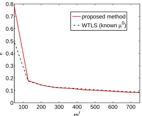
Surprisingly, the difference between the estimation accuracy of the parameter of interest X for the proposed and weighted total least squares estimators is much smaller than the one for the parameters λ₁0 and λ₂0. Figure 2 shows the average relative estimation error

e := 1 100

100

∑

i=1

kX−Xˆ(i)k kXk ,

experi-ment. For sample sizes m above 150, the two estimators achieve almost the same ac-curacy (although the acac-curacy in theλ₁0andλ₂0estimates is higher for the weighted total least squares estimator).

Finally, we show in Figure 3 the function f(m0)that is used for the estimation of the turnover point in the case when the sample size is m=1500. The sharp maximum of f(m0)at m0=750 shows that in the example the proposed method allows to detect correctly the turnover point. The example, however, has well separated classes, with difference in both mean and variance. Simulations suggest that equal means of the clusters makes the turnover point estimation harder even if the variances of the clusters still differ. In such cases, the function f(m0)has many local maxima.

100 200 300 400 500 600 700

8 8.5 9 9.5 10 10.5

true value proposed method

WTLS (known µ0)

PSfrag replacements

m0

ˆλ1

100 200 300 400 500 600 700

12 12.5 13 13.5 14 14.5 15 15.5 16

true value proposed method

WTLS (known µ0)

PSfrag replacements

m0 ˆ

λ1

ˆλ2

Fig. 1. Average values of the noise variance estimates ˆλ1 and ˆλ2as a function of half the

sample size m0. The dashed lines indicate the true values.

100 200 300 400 500 600 700

0 0.1 0.2 0.3 0.4 0.5 0.6 0.7 0.8

proposed method

WTLS (known µ0)

PSfrag replacements

m0

e

200 400 600 800 1000 1200 1400 250

300 350 400 450 500

true value of m₁

PSfrag replacements

m0

f

(

m

0 )

est. function f

Fig. 3. Estimation of the turnover point m1. 8 Conclusions

We considered a multivariate errors-in-variables model AX = B, with finite de-pendent rows. The total error covariance structure of data matrix D= hA B

i

was known up to two scalar factors. We supposed that the row data are clustered into two groups, with essentially different second empirical moments. Based on a matrix D>D, we constructed the consistent estimators of the scalar factors and X .

The clustering assumption is crucial for the consistency. In practical applications, given a matrix D we first have to check a statistical hypothesis about the presence of a change point. If the hypothesis is accepted then we have to divide the rows of D in two clusters, according to the optimization problem (8)–(9). After that we can compute the corresponding estimators.

The idea seems plausible for practical system identification. It can be easily gener-alized to N>2 uncorrelated blocks of the error matrix and N unknown scalars, but then we need N clusters as well, that correspond to N−1 change points in the data.

Acknowledgments

Prof. Alexander Kukush is a full professor at the Kiev National Taras Shevchenko Univer-sity, Kiev, Ukraine. He is supported by a senior postdoctoral fellowship from the Depart-ment of Applied Economics of the Katholieke Universiteit Leuven. Dr. Ivan Markovsky is a lecturer at the School of Electronics and Computer Science, University of Southampton, UK and Prof. Sabine Van Huffel is a full professor at the Electrical Engineering Deperat-ment of the Katholieke Universiteit Leuven, Belgium.

666, several PhD/postdoc & fellow grants; Flemish Government: FWO: PhD/postdoc grants, projects, G.0078.01 (structured matrices), G.0407.02 (support vector machines), G.0269.02 (magnetic resonance spectroscopic imaging), G.0270.02 (nonlinear Lp approximation), G.0360.05 (EEG signal processing), research communities (ICCoS, ANMMM); IWT: PhD Grants; Belgian Federal Science Policy Office IUAP P5/22 (‘Dynamical Systems and Con-trol: Computation, Identification and Modelling’); EU: PDT-COIL, BIOPATTERN, ETU-MOUR.

The authors are grateful to Prof. H. Schneeweiss for fruitful discussions.

A Proof of Theorem 1

Let m1=κm,κ∈[r1,r2].Define a functionΦt(κ),κ ∈[r1,r2],related to F(m1):

(a) Φt(_mk) =F(k)if r1≤_mk ≤r2;

(b) let k1and k2be the smallest and largest numbers satisfying the latter inequality,

then we setΦt(x) =Φt(k_m1), x∈[r1,k_m1],andΦt(x) =Φt(k_m2), x∈[k_m2,r2];

(c) for x∈(_mi,i+_m1), k1 ≤i≤k2,we define Φt(x) by linear interpolation ofΦt(_mi)

andΦt(i+_m1).

Now, ˆm1=κˆm,and

Φt(κˆ) = max r1≤κ≤r2

Φt(κ). (A.1)

Using (5) and (7), it is possible to show that these existΩ0, Pr(Ω0) =1,such that

for eachκ∈[r1,r2]andω ∈Ω0,

Φt(κ)→Φ∞(κ):=ϕ(κ)σ1(E uu>−E vv>), as t→∞,

where

ϕ(κ):=

     

    

1−r

1−κ, if r1≤κ≤r

r

κ, if r≤κ≤r2.

Moreover Ω0 can be constructed in such a way that for eachω ∈Ω0 andδ >0,

the functions{Φt(κ), t≥1}are equicontinuous on[r1,r−δ]∪[r+δ,r2].Thus for

ω ∈Ω,

Φt(κ)→Φ∞(κ), as t→∞, (A.2)

uniformly on[r1,r−δ]∪[r+δ,r2],andΦ∞∈C[r1,r2].Due to condition(cl2)the

limit functionΦ_∞(κ)has a unique maximum atκ0=r.Then (A.1) and (A.2) imply

that for eachω ∈Ω0,κˆ →κ0,as t→∞.Therefore

ˆ m1

B Proof of Theorem 2

B.1 Behavior of Qc(λ0)

We have

Qc(λ0) =

2

∑

k=1

p

∑

i=1

µ2

ik(λ0) +cksinΘ(λ0)k2. (B.1)

By Lemma 1 and Theorem 1, for k=1,2

° ° ° °

1 mk(t)

Ψ(k)

c (λ0)−

1 mk(t)

¯

D>(k)_D¯_(k)

° ° ° °

→0, as t→∞, a.s.

We haveµi ¡_¯

D>(k)D¯(k)/mk(t) ¢

=0, 1≤i≤p, and by Lemma 2,

lim

t→∞µp+1

µ

1 mk(t)

¯

D>(k)D¯(k)

¶

>0, a.s.

Then a.s.

lim

t→∞

2

∑

k=1

p

∑

i=1

µ2

ik(λ0) =0,

and by Wedin’s theorem, see Steward and Sun (1990), Theorem 4.1, p.260,

ksinΘk(λ0)k →0, as t→∞, a.s.; k=1,2.

HereΘk(λ0)is the diagonal matrix of canonical angles between Lp(Ψc(k)(λ0)/mk(t))

and Lp(D¯>(k)D¯(k)/mk(t)), and Lpdenotes the span of the p eigenvectors. Now,

Lp(D¯>(1)D¯(1)/m1(t)) =Lp(D¯>(2)D¯(2)/m2(t)) =span(z1, . . . ,zp),

where

h

z1 . . . zp i

=h−XIp i

. Therefore ksinΘ(λ0)k →0, as t →∞, a.s., and from (B.1) we obtain

Qc(λ0)→0, as t→∞, a.s.

By the definition of ˆλ, this implies that

B.2 λˆ is eventually bounded

Now we want to construct such a nonrandom L>0 that eventually

kλˆk ≤L. (B.3)

First from (B.2) we have for anyε0>0 that

2

∑

k=1

p

∑

i=1

µ2

ik(λˆ)≤ε0 eventually. (B.4)

We have by Lemma 1 and Theorem 1 that

¯ ¯ ¯ ¯

1 m1(t)

Ψ(1)

c (λˆ)−

1 m1(t)

Ψ(1)

ls (λˆ)

¯ ¯ ¯ ¯

→0, as t →∞, a.s. (B.5)

Here

Ψ(1)

ls (λ):=D¯

>₍

1)_D¯₍₁₎₋





(λ1−λ₁0)W1(1) 0

0 (λ2−λ20)W2(1)



, λ:= (λ1,λ2)∈[0,∞)×[0,∞).

We have for m1=m1(t):

tr ³

X_ext>(Ψ(_ls1)(λˆ)/m1)Xext

´

=−tr ³

(λˆ1−λ10)X1>

¡

W1(1)/m1

¢

X1+ (λˆ2−λ20)X2>

¡

W2(1)/m1

¢

X2

´ .

Suppose that ˆλ1−λ₁0>L0, where L0>0. Then

tr ³

X_ext>(Ψ(_ls1)(λˆ)/m1)Xext

´

≤ −L0tr¡X1>

¡

W1(1)/m1¢X1¢+const·λ20.

But from (f) and (g),

lim inf

t→∞ tr

¡

X₁>(W1(1)/m1)X1

¢ >0.

Therefore for L0large enough and all t ≥t0, we have

tr³X_ext>(Ψ_ls(1)(λˆ)/m1)Xext

´

≤ −1.

This implies that µ1

¡Ψ(1)

ls (λˆ)/m1

¢

<0 and separated from 0. Then from (B.5) we have thatµ1

¡Ψ(1)

c (λˆ)/m1

¢

is also negative and separated from 0 for t≥t1(ω), a.s.

But this contradicts (B.4). Thus for large enough nonrandom L0, ˆλ1−λ₁0 ≤L0,

eventually. Similar inequality can be shown for ˆλ2−λ₂0, based on condition (f) for

B.3 Consistency

We fixΩ0, Pr(Ω0) =1, such that for allω∈Ω0,kλˆ(ω)k ≤L, for all t≥t0(ω). Fix

ω ∈Ω0. We consider a bounded sequence

{λˆ(ω;t): t≥t0(ω)} (B.6)

and want to show that it converges toλ0, as t →∞. Let

{λˆ¡ω

;t(q)¢

, q≥1}

be any convergent subsequence. It means that t(q)→∞, and

lim

q→∞

ˆ

λ¡

ω;t(q)¢

=λ∞,

for certainλ∞∈R2. To prove the desired convergence (B.6), it suffices to show that

λ∞_=λ0_.

Let

M(k)(t) =diag(µ1k,µ2k, . . . ,µpk)

and Z(k)(t) be a matrix

h

f₁(k)(t) . . . fp(k)(t) i

, of which the columns are the first

eigenvectors ofΨ(ck)(λˆ)/mk(t); these columns form an orthogonal basis for Lpk(λˆ).

Due to (B.2), M(k)(t)→0, as t→∞, and we can assume that

° ° °Z

(1)_(t)−Z(2)_(t)°°

°→0, as t→∞. (B.7)

We have

1 mk

Ψ(k)

c (λˆ)Z(k)(t) =M(k)(t)Z(k)(t). (B.8)

We set here t =t(q). We may and do assume that Z(k)¡t(q)¢

→Z(∞k), as q→∞, k=1,2. (Otherwise we should consider a convergent subsequence). From (B.7) we obtain Z_∞(1)=Z_∞(2)=: Z_∞, and from (B.8) we have, since

sup

kλk≤L ° ° ° °

1 mk(t)

Ψ(k)

c (λ)−

1 mk(t)

Ψ(k)

ls (λ)

° ° ° °

→0, as t→∞,

that

1 mk(t(q))

Ψ(k)

ls (λ∞)Z∞→0, as q→∞, k=1,2.

Hence

µ

1 m1(t(q))

Ψ(1)

ls (λ∞)−

1 m2(t(q))

Ψ(2)

ls (λ∞)

¶

Using condition (g), we obtain

µ

1 m1(t(q))

¯

D>(1)_D¯₍₁₎₋ 1 m2(t(q))

¯

D>(2)_D¯₍₂₎

¶

Z_∞→0, as q→∞.

But then from condition(cl2)similarly to Lemma 2 we obtain that Z∞=

h

z∞₁ . . . z∞_p

i

with span(z∞₁, . . . ,z∞_p) =span(z1, . . . ,zp). Thus in (B.8) we have

1 mk(t(q))

Ψ(k)

ls (λ∞)Xext→0, as q→∞, k=1,2.

Thus





(λ₁∞−λ0

1)W1(1)/m1(t(q)) 0

0 (λ₂∞−λ0

2)W2(1)/m2(t(q))



Xext→0

and

(λ_j∞−λ0_j)tr¡X>_j Wj(1)Xj/mj(t(q)) ¢

→0, as t→∞, j=1,2.

But then conditions (f) and (g) imply that λ∞_j =λ0

j, j=1,2. Thus any

conver-gent subsequence of the bounded sequence (B.6) converges to λ0, therefore the sequence (B.6) itself converges toλ0. This convergence holds for allω∈Ω0, with

Pr(Ω0) =1, therefore ˆλ →λ0, as t→∞, a.s.

C Proof of Theorem 3

By Theorem 2

° ° ° °

1

m(t)(Hˆ −D¯

>_D¯)

° ° ° °

→0, as t→∞, a.s.

We have

µ1

µ

1 m(t)D¯

>_D¯

¶

=. . .=µp µ

1 m(t)D¯

>_D¯

¶

=0,

and by condition (h) and Lemma 2,µp+1

¡_¯

D>D¯/m¢is separated from 0, as t→∞. Moreover, the kernel equals

Lp µ

1 mD¯

>_D¯

¶

=span(z1, . . . ,zp).

Thus ˆX is also uniquely defined eventually. Since





X −Ip



= h

z1 . . . zp i

,

fromΘ→0 a.s., we obtain that ˆX→X , as t→∞, a.s.

References

[1] J.C. Aq˜uero, and G.C. Goodwin (2006). Idetifiability of errors in variables dynamic systems. 14th IFAC Sympsium on System Identification, Newcastle, Australia.

[2] B. Anderson (1985). Identification of scalar errors-in-variables models with dynamics. Automatica, 21, 625–755.

[3] R. Carroll, D. Ruppert, and L. Stefanski (1995). Measurement Error in Nonlinear Models. Chapman & Hall/CRC, London.

[4] G. Cirrincione, S. Van Huffel, A. Premoli, and M.-L. Rastello (2001). Iteratively reweighted total least squares algorithms for different variances in observations and data, In Advanced Mathematical & Computational Tools in Metrology V(eds.P.Ciarlini et al.), 77–84, World Scientific, London.

[5] P. Doukhan (1934). Mixing. Properties and Examples, Springer–Verlag, New–York. [6] R. Frisch (1934). Statistical confluence analysis by means of complete regression

systems. Technical Report 5. Univ. of Oslo, Economics Institute.

[7] A. Kukush and S. Van Huffel (2004). Consistency of elementwise-weighted total least squares estimator in a multivariate errors-in-variables model AX=B. Metrika, 59,75– 97.

[8] A. Kukush, S. Zwanzig (2001). About the adaptive minimum contrast estimator in a model with nonlinear functional relations. Ukrainian Mathematical Journal, 53, 1145– 1452.

[9] A. Kukush, I. Markovsky, and S. Van Huffel (2005a). Estimation in a linear multivariate measurement error model with clusterin in the regression, Technical Report 05-170, Dept. EE, K.U.Leuven.

[10] A. Kukush, I. Markovsky, and S. Van Huffel (2005b). Consistency of the structured total least squares estimator in a multivariate errors-in-variables model. J. of Stat. Planning and Inference, 133,315–358.

[12] I. Markovsky, A. Kukush, and S. Van Huffel (2006). On errors-in-variables estimation with unknown noise variance ratio, In the proceedings of the 14th IFAC Symposium on System Identification, pages 172–177, Newcastle, Australia, 2006.

[13] B. De Moor (1988). Mathematical concepts for modeling of static and dynamic systems. PhD thesis, Dept. EE, K.U.Leuven, Belgium.

[14] J. A. Nelder and R. Mead (1965). A simplex method for function minimization. Computer J., 7, 308–313.

[15] A. Pakes (1982). On the asymptotic bias of Wald-type estimators of a straight line when both variables are subject to error. International Economic Rewiev, 23, 491– 497.

[16] G. Stewart and J. Sun (1990). Matrix Perturbation Theory. Academic Press, Boston. [17] T. Söderström, U.Soverini, and K.Mahata (2002). Perspectives on errors-in-variables

estimation for dynamic systems, Signal Processing, 82, 1139–1154.