Comparison of Spectra Using a Bayesian Approach An Argument Using Oil Spills as an Example

Comparison of Spectra Using a Bayesian

Approach. An Argument Using Oil Spills as an

Example

Jianfeng Li and D. Brynn Hibbert*

School of Chemistry, University of New South Wales, Sydney, NSW 2052, Australia

Steven Fuller, Julie Cattle, and Christopher Pang Way

Environmental Forensic and Analytical Science, Department of Environment and Conservation, New South Wales Environment Protection Authority, Lidcombe, NSW 2141, Australia

The problem of assigning a probability of matching a number of spectra is addressed. The context is in en-vironmental spills when an EPA needs to show that the material from a polluting spill (e.g., oil) is likely to have originated at a particular site (factory, refinery) or from a vehicle (road tanker or ship). Samples are taken from the spill, and candidate sources and are analyzed by spec-troscopy (IR, fluorescence) or chromatography (GC or GC/MS). A matching algorithm is applied to pairs of spectra giving a single statistic (R). This can be a point-to-point match giving a correlation coefficient or a Euclid-ean distance or a derivative of these parameters. The distributions of R for same and different samples are established from existing data. For matching statistics with values in the range{0,1}corresponding to no match (0) to a perfect match (1) aβdistribution can be fitted to most data. The values ofRfrom the match of the spectrum of a spilled oil and of each of a number of suspects are calculated and Bayes’ theorem is applied to give a prob-ability of matches between spill sample and each candi-date and the probability of no match at all. The method is most effective when simple inspection of the matching parameters does not lead to an obvious conclusion; i.e., there is overlap of the distributions giving rise to dubiety of an assignment. The probability of finding a matching statistic if there were a match to the probability of finding it if there were no match, expressed as a ratio (called the likelihood ratio), is a sensitive and useful parameter to guide the analyst. It is proposed that this approach may be acceptable to a court of law and avoid challenges of apparently subjective opinion of an analyst. Examples of matching the fluorescence and infrared spectra of diesel oils are given.

When a polluted site is found some questions may be asked including the following; “What is the likely composition of the spill?”, “Which analytical techniques can be used to best effect?”,

“Is the spill dangerous or harmful to the environment?”, and if there are suspects as the source of the spill, “Who can be prosecuted?” A successful outcome depends on the reliability of the answers to these questions, which are based on appropriate sampling, selection of methodology, processing, and interpretation of the experimental data. In some cases, when there is an immediate knowledge of the nature of the spill and there is only one potential defendant, the subsequent analysis and conclusion of origin may be incontestable. Even when there are a number of suspect sources, if the suspect samples differ significantly from each other, many analytical techniques seem to work well to give the correct match. At present, an Environmental Protection Authority (EPA) may use two or three independent analytical techniques to establish and then confirm the match. However, when several suspects have a strong resemblance to each other or when no suspects resemble the spill, difficulties arise. In the first case, assigning culpability is difficult to make and, with good defense casting doubt on the true identity of the source, difficult to sustain in a court of law. A professional analyst may refuse to make any firm decision. In the second case, it is better to know, with a scientifically established probability, that a candidate did not contribute to the spill so that it may be removed from the investigation.

It is very common in oil spill cases that many similar suspects are investigated. For an oil spill accident, it is quickly obvious that the spill is oil of a particular type (e.g., crude or diesel), but it can be difficult to find the guilty source because the differences between different oils of the same type are subtle, and weathering also causes changes in the properties of spilled oil. Consider a spill that is found on a beach around which there are a few oil refineries, all producing diesels. After some analysis, the EPA knows the spill is diesel but may not be able to find a conclusive “signature” of the polluting refinery. Present standard methods attempt to make general classifications by following a flowchart of comparisons that lead to results expressed as a “match”, “probable match”, “no match”. This is done, for example, in the ASTM matching of oil samples by IR.1_{When analytical techniques}

* To whom correspondence should be addressed. E-mail: b.hibbert@ unsw.edu.au. Telephone: +61 2 9385 4713. Fax: +61 2 9385 6141.

(1) ASTM.D 3414-98; American Society for Testing and Materials: Philadelphia, 1998.

Anal. Chem.2005,77,639-644

are used that give unique signals at a particular wavelength, mass, or time then matching can be decided by whether a signal is observed within a prescribed window of the value to be matched. For example,(10% has been used as the criterion of a match between samples using GC/MS.2_{Usually, however, there is no} clear-cut signature and the analyst relies on experience to conclude whether, on the weight of evidence, a match is likely.

With repeated measurement of a number of samples, statistics can be used to test the similarity by setting up a null hypothesis (H0) that is based on an assumption such as “the spectrum of the spill sample and suspect sample come from the same source”. The question is then to choose a suitable statistic with a known distribution. In using a traditional frequentist approach, there is the danger of interpreting an acceptance ofH0as confirmation of a match. When rejectingH0at typically the 95% probability level, the analyst is making the decision that the samples will be declared different if the probability of the test statistic or a more extreme value given the null hypothesis falls below 0.05. A probability of finding the data givenH0of only 5% does not inspire confidence that a match has been supported. Data with a large standard deviation may not easily allow rejection ofH0, leading to a conclusion of “not proven different” rather than “proved the same”. It is also not easy to extend the statistics to multiple samples. Matches must be done pairwise. (Analysis of variance does not help here as if the grouping factor is “sample type”, a knowledge that some sample types do not match is not helpful.) Furthermore, conventional statistical wisdom would seem to support asserting that the suspect pattern that “most closely” matches the spill pattern (i.e., has the greatest probability given

H0) actually “identifies” the source of the spilled oil.

What is required, regardless of the analytical method em-ployed, is a measure of the analyst’s confidence in each hypo-thesized match and also in the absence of any match. It is imperative to be able to assign a statistically sound probability to each spill-suspect match based upon a priori knowledge of (a) the precision of the analytical method and (b) the distribution functions of matched oils and different oils for the matching statistic over all samples in the case.

Bayesian statistics is often seen as a complement (or competi-tor) to frequentist statistics, which is more usually seen in analytical chemistry. Briefly, Bayes’ theorem gives the probability of an hypothesis given the evidence, in contrast to a frequentist approach that calculates the probability of the evidence (usually a test statistic) given the acceptance of the hypothesis.3,4_{It has} found many uses in analytical chemistry and particularly in forensic science where the probability of an event, for example, the probability that a sample of DNA came from a suspect, can be useful.5-7

In this paper, we shall show that a Bayesian analysis which relies on mutually exclusive and exhaustive outcomes (i.e., all

probabilities sum to 1) gives such a desired probability for matching any two samples and the case in which no samples match at all. It builds on the approach in a conference paper of Killeen and Chien,8_{that appears not to have received any further} attention.

THEORY

Matching Statistics.For spectra or chromatograms that are stable in the frequency or time axis (i.e., peaks appear consistently at the same wavelength or time), a point-to-point match may be made between two spectra. A suitable interval is chosen to account for any small uncertainty in the position of points on the abscissa and to deliver a useful number of data, and within this interval, the signal may be integrated to give additional stability. For fluorescence spectra, matches such as the correlation coefficient and the sum of the Euclidean distances between points have been shown to be effective.9-11_{The choice of method is based on the} utility of the measure in distinguishing between the same and different samples. Here we use the square of the correlation coefficient to illustrate the method.

where Cov(A1,A2) is the covariance of the vectors of the spectra to be matched (measured as emission intensity, transmittance, or absorbance) andsis the standard deviation of a spectrum. We have shown that it may be advantageous to take differences between measurements at successive wavelengths before applying eq 1, i.e.,Ais replaced by∆A, where a component of the vector ∆Ai)Ai+1-Ai.9This procedure compensates for baseline drift in the spectra. The closer two spectra are, the nearerRis to 1. For two vectors that have no linear correlation, R ) 0. An advantage of a simple statistic such as the correlation coefficient is that it can be applied to vectors of absorbances, peak heights, peak areas, or counts and so may be used with any analytical technique that gives an output as a function of an ordering variable such as wavelength, time, or mass.

Distributions of Matching Statistics.At the heart of the method we propose is knowledge of the distributions of the matching statistic for samples that do indeed come from the same origin and those that do not. How each set of samples that define these distributions is chosen will determine the outcome of any matching calculation. Two issues must be addressed: to what extent the set is restricted based on prior knowledge of the oils and if weathering or other changes will be taken into account. If the spill is clearly identified as a diesel, then it would be a mistake to conduct the analysis using samples of diesels, kerosene, and crude oils. Restricting the set to diesels will allow finer distinctions to be made among diesels. The distributions will then be specific for diesels, of course. It is also likely that the analytical data will be collected on a single instrument, again restricting the use of (2) Worrall, R. D.Oil Spill Identification; Australian Government Analytical

Laboratories: Cottesloe, WA, 1996. (3) Malakoff, D.Science1999,286, 1461-1461.

(4) Casella, G.Chemom. Intell. Lab. Syst.1992,16, 107-125.

(5) Robertson, B.; Vignaux, G. A.Interpreting Evidence: Evaluating Forensic Science in the Courtroom; John Wiley & Sons Inc: Chichester, 1995. (6) Curran, J. M.; Hicks, T. N.; Buckleton, J. S.Forensic Interpretation of Glass

Evidence; CRC Press: London, 2000.

(7) Evett, I. W.; Weir, B. S.Interpreting DNA Evidence: Statistical Genetics for Forensic Scientists; Sinauer Associates, Inc.: Sunderland, MA, 1998.

(8) Killeen, T. J.; Chien, Y. T.Proc. Workshop Pattern Recognition Appl. Oil Identif. 1977; pp 66-72.

(9) Li, J.; Fuller, S.; Cattle, J.; Pang Way, C.; Hibbert, D. B.Anal. Chim. Acta 2004,514, 51-56.

(10) Baumann, K.; Clerc, J. T.Anal. Chim. Acta1997,348, 327-343. (11) Tanabe, K.; Saeki, S.Anal. Chem.1975,47, 118-122.

R)

(

1sA2

)

2

the information to spectra collected on that instrument. Second, if weathering is to be accounted for, then the set of similar spectra must include a range of weathered samples. This will broaden the distribution with attendant overlap with the dissimilar distribu-tion. It is desirable, and may be necessary, to find a similarity measure that accounts for weathering (i.e., gives a high match statistic even though the spectra are apparently different) al-though, for cases investigated by us, this has not been the case. Because we are dealing with mixtures of essentially similar chemicals, correlation between two spectra of a common type of oil will be expected to be reasonably high. Differences between samples of the same oil will reflect any changes in the oil itself (weathering), sampling including the thickness of an IR sample, and instrumental variance.

Estimating the distributions is aided by the large number of pairwise squared correlation coefficients that may be obtained from a set of spectra. For N different oils each sampled and measuredmitimes, there will beNs)∑i)1

i)N

(mi(mi-1)/2) values ofRfor the same oils, and (∑i)1

i)N

mi(∑i)1

i)N

mi-1)/2)-Nsvalues for different oils. It is unlikely that the distribution of the values ofRwill be normal, but we will show it is possible to fit them to

βdistributions, generate a probability density function (pdf) by kernel density estimation, or simply histogram the available data and use the normalized numerical frequency of a bin as the pdf. In practice, an EPA will have a great amount of historical data that can be used to give good estimates of the distributions.

Bayes’ Theorem Applied to Matching. Bayes’ theorem allows calculation of the probability of an hypothesisHibased on available evidenceE. This is written Pr(Hi|E). In our case, the hypothesis could be that two samples were from the same source, and the evidence could be a correlation coefficient calculated from spectra or a comparison between two chemical measurement results. According to Bayes, for N competing and mutually exclusive hypotheses

Pr(E|Hi), the probability of finding the evidenceEgiven the truth of the hypothesisHi, is known as the likelihood ofHiand is the probability that is often calculated in statistical tests in chemistry, when the “null hypothesis” is assumed and the probability of the value, or more extreme value, of the observed statistic, for example, a Student t value, is calculated from measurement results. Note that this is not the same as Pr(Hi|E). Pr(Hi) is the prior probability of the hypothesis before any evidence is considered. In the absence of any other prior knowledge of the system, each Pr(Hi) can be set as 1/N. This term then cancels in the equation. The form of eq 2 ensures that∑j)1

j)N_Pr(

Hj|E))1. The use of so-called “flat priors” is well known, although the validity of the assumption of equal probability may often be challenged.

The simplest case, that of matching two spectra, is discussed first. Suppose we have two samples that are to be compared and from a pair of spectra we have calculated a similarity indexRwith resulting valuer. The two hypotheses are H, that the two samples

come from a common source, and Hh that they do not. Equation 2 for the hypothesisHbecomes

To determine the likelihood probabilities, we need to know the distribution ofRfor samples that match and for those that do not. The distributions of values of Rfor matched samples and different samples may be known from many measurements, and they are likely not to be normally distributed. Hopefully the similar samples will have values ofrnear 1 and the dissimilar samples will havervalues distributed across lower values. Figure 1 is a schematic of plausible distributions. The pdf ofR of matching spectra will be termedS(R), and the pdf ofRof different spectra will be termed D(R) as shown in the figure. Two particular samples (let them be a and b) to be compared will yield a value of the similarity indexR)ra.b. If Pr(H))Pr(Hh))0.5, for the hypothesis that the samples match, Equation 3 becomes

The method is extended to multiple comparisons in a straight-forward way. For example, if a spill sample is compared with three candidate source samples, there are four hypotheses, three for matching with sources 1, 2, and 3, respectively (H1,H2,H3), and for a match with none (Hh). There are three squared correlation coefficients between the spill and each of the suspect sources,r1,

r2, r3, each having a corresponding pdf of being a match, S(r1), S(r2), S(r3), or not matching,D(r1),D(r2),D(r3). We set Pr(H1)) Pr(H2))Pr(H3))Pr(Hh))1/4, which cancels in eq 2. Therefore, taking an hypothesized match with the first suspect (H1) as an example

If the results are to be used for forensic purposes, a useful statistic that the courts can use in the case where there is a simple choice (match/no match) is the likelihood ratio

Pr(Hi|E))

Pr(E|H_i)Pr(H_i)

∑

j)N

Pr(E|H_j)Pr(H_j)

(2)

Figure 1. Sketch of distributions of a similarity statistic between two spectra for samples of common origin (dashed line labeledS(R)) and different origin (solid line labeledD(R)).

Pr(H|r)) Pr(r|H)Pr(H)

Pr(r|H)Pr(H)+Pr(r|Hh)Pr(Hh) (3)

Pr(H|ra.b))

S(ra.b)

S(ra.b)+D(ra.b)

(4)

Pr(H₁|r₁r₂r₃))S(r₁)D(r₂)D(r₃)/(S(r₁)D(r₂)D(r₃)+

D(r₁)S(r₂)D(r₃)+D(r₁)D(r₂)S(r₃)+D(r₁)D(r₂)D(r₃)) (5)

LR)Pr(r|H)

the ratio of the probabilities of the statistic given a match or no match. If the a priori probabilities are equal, this ratio is also the ratio of the posterior probabilities

because Pr(H))Pr(Hh) and so cancel in eq 3.

The likelihood ratio (eq 6) is how many times more likely the evidence is given the matching hypothesis than the alternative hypothesis of no match, while eq 7 gives how many times the hypothesis that there is a match is supported by the evidence, compared with the alternative hypothesis that there is no match. Under the assumption of equal a priori probabilities, the two ratios are the same, but if the posterior probability is required, the assumptions about the a priori probabilities must be clearly stated and justified. Courts have often been more comfortable with likelihood ratios, which do not need to determine prior probabilities.5,12-14_{If the Bayesian approach is accepted, eq 7 is} to be preferred because it offers information about the hypotheses given the evidence, rather than the evidence assuming the hypothesis.

EXPERIMENTAL SECTION

Oil Samples.For the first example using fluorescence spectra, two similar, but not identical, diesel samples were provided by the New South Wales Environment Protection Authority (NSW EPA). These are typical diesels used as automotive fuel.

The second series of samples is from an oil spill in Sydney found in a recreational park and golf course and analyzed by infrared spectroscopy. Table 1 gives the origins and naming scheme used in the text.

The database of matching and nonmatching infrared spectra was built up from samples held by the NSW EPA.

Analysis.Fluorescence spectra were obtained on a Perkin-Elmer model LS-50B luminescence spectrophotometer with a personal computer using FL-WinLab version 2.01 (The Perkin-Elmer Corp., Norwalk, CT). The oil solutions were prepared using spectroscopic pure cyclohexane as solvent. A known volume of pure sample was made up to the desired volume fraction with cyclohexane. The excitation wavelength was 245 nm. The slit widths of excitation and emission beams were 10 and 2.5 nm,

respectively, and the scan speed was 120 nm/s. The emission spectrum between 300 and 500 nm was collected at 1-nm intervals and was normalized to the maximum of the spectrum. More information can be found in ref 15.

Infrared spectra of the “golf course” spill were collected on a Fourier transform infrared spectrophotometer (Excalibur FTS 3000, Bio-Rad). The oil samples were analyzed under the same conditions using the same KBr cell, which was cleaned between samples, and the spectra were recorded from 4000 to 650 cm-1_{. A total of 32 scans at a resolution of 4 cm}-1_{were collected} and averaged for the background and for each sample. A 0.05-mm spacer in the cell ensured consistent thickness of the oil sample.

Calculations.In the example using fluorescence spectra, each oil was analyzed 15 and 17 times, respectively, giving 105+136 )_{241 and 496}-₂₄₁)_{255 pairs of similar spectra and pairs of} dissimilar spectra, respectively. Difference correlation statistics (eq 1 applied to differences of adjacent emission intensities for each spectrum,Rd) were calculated for each pair of spectra. For each matching method, the probability distributions of the statistics (same spectra and different spectra) were calculated by fitting to aβfunction. From these distributions (S(R) andD(R) for each matching statistic), the Bayesian probability distribution of a match was calculated.

A similar approach was taken with the golf course samples. The distributions of the similarity indices of comparisons of FT-IR spectra of 18 kinds of oil and their weathered derivatives in the wavenumber range of 900-700 cm-1_{gave (with replicates)} 5450 comparisons between different oils and 125 comparisons between same oils. Various matching statistics were calculated, but here only the difference correlation squared as defined above is shown and discussed.

RESULTS

Fluorescence Spectra.Figure 2 shows fluorescence spectra of the two diesel oils. Each spectrum was of an independent sample, and thus, the variability arises from the sample preparation and measurement uncertainty. For every pair of spectra from the same source (A with A and B with B), the squared difference correlation coefficient was calculated and similarly for every pair of dissimilar spectra (A with B). Figure 3 shows histograms of the squared difference correlation coefficients with overlaid best-(12) Robertson, B.; Vignaux, G. A.N. Z. Law J.1992,9, 315-317.

(13) Champod, C.; Girod, A.; Sjerps, M. The Meaning of Conclusions in the Identification. Context, In First European Meeting of Forensic Science; Lausanne, 1997.

(14) Champod, C. The Inference of Identity of Source: Theory and Practice. In First International Conference on Forensic Human Identification in the Next Millennium; The Forensic Science Service; London, 1999.

(15) ASTM.D 3650-93; American Society for Testing and Materials.: Phila-delphia, 1993.

Table 1. Details of Oil Spill Samples

sample descriptor origin

G1 oil contamination of golf course R1, R2 samples from river near golf course

R3 sample from boom across creek used

to contain oil spill from rail yard Y2 oil from culvert in rail yard Y1 waste oil well in rail yard

Pr(H|r)

Pr(Hh|r) (7)

fitβdistributions. It is seen that oil A gave poorer self-matching statistics than oil B, but both distributions covered greaterRvalues than the distribution of nonmatching R values. The figure illustrates how a matching statistic on its own is not a guide to whether the spectra are from the same oil. Different diesels have values ofRgreater than 0.93 in this case, because of their innate similarity. However when spectra of the same oil are taken, even greater values ofRare obtained. Exploring the hypotheses that a givenris evidence of a match with A or not A, or thatris evidence for a match with B or not B, gives probabilities from eq 3 for the relevant match (Figure 4). The greater extent of overlap of the distribution of spectra of different oils with that of A is reflected in the greater region of uncertainty. With oil B, however, the transition from a probability Pr(HB|r<0.975)≈0 for (i.e., Pr-(HhB|r<0.975)≈1) to Pr(HB|r>0.977)≈1 shows that there will rarely be any question about the correct assignment. The transition fromrnot supporting the match to supporting the match is even more obvious when the likelihood ratios are plotted (Figure 5).

The analysis allows exploration of the case in which there are three possible outcomes of a match; the unknown matches A, matches B, or matches neither. The spectrum of the unknown is compared with that of A and B and the statistic rA and rB calculated. From the distributions, the likelihoods Pr(rArB|HA), Pr-(rArB|HB), and Pr(rArB|Hh) are calculated, where Hh represents the hypothesis that there is no match at all. The probability that

the unknown sample matches A is thus

whereSAis from the distribution ofRfor matching A,SBfrom matching B andDfrom the distribution ofR values of spectra that do not match.

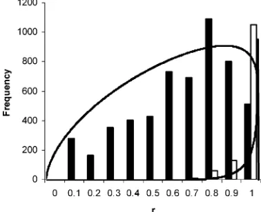
Infrared Spectra. Matching infrared spectra from diesel samples shows a much greater overlap between the squared difference correlation coefficients (r) of nonmatched samples and matched samples (Figure 6). The distribution ofrfor nonmatched samples spans nearly the entire allowed range (0-1). The lowr

tail of the distribution of matched samples arises from weathering effects when samples have been artificially weathered to different degrees, although still classed as the same sample. With the oil spill data from samples described in Table 1, the infrared spectrum of each sample was matched against that of all the others. The squared difference correlation coefficients are given in Table 2. Although there are a number of samples, we are only interested Figure 3. Histograms and overlaidβdistributions of the squared

difference correlation coefficients for the spectra shown in Figure 2. Solid bars, different samples (A with B); open bars, samples of oil A (A with A); gray bars, samples of oil B (B with B).

Figure 4. Probability of a match to A (solid line) or B (dashed line) calculated from distributions with squared difference correlation coefficient.

Figure 5. Likelihood ratios Pr(A)/Pr(Ah) (filled circles) and Pr(B)/Pr-(Bh) (open circles) calculated from the probabilities shown in Figure 4.

Figure 6. Histograms and overlaidβdistributions of the squared difference correlation coefficients of infrared spectra of diesel samples. Solid bars, different samples, Beta(1.74,1.13); open bars, matching samples, Beta(10.22,0.56). Note the frequencies of the matching samples have been multiplied by 10 for clarity.

Pr(HA|rArB))

Pr(r_ArB|H_A)Pr(H_A)

Pr(r_ArB|H_A)Pr(H_A)+Pr(r_BrA|H_B)Pr(H_B)+Pr(r_ArB|Hh)Pr(Hh)

) SA(rA)D(rB)

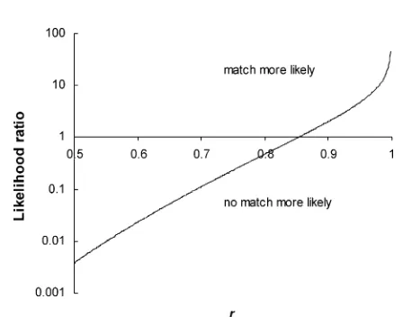
in a one-to-one match, and so the simple equation (eq 4) can be used. Figure 7 shows the likelihood ratio as a function ofr. It is only whenrapproaches 1 that it becomes distinctly more probable that there is a match. Table 3 gives the probabilities of a match associated with the values ofrin Table 2 (upper triangle), and the likelihood ratios (lower triangle). Note that the greatest ratios, matching R1 to R2 and R3 to Y2, happen to be numerically equal by the chance of equalr.

DISCUSSION

In the golf course example, there was some prima facie evidence that the spill came from the railyard. There had been an oil spill, albeit contained, but there was no clear trail to the golf course. It is seen from the Bayesian analysis that there is evidence for a match between samples R1 and R2, which were collected from the same site (a river flowing past the golf course) and between Y2, the rail yard culvert, and R3, the boom across

the river outside the rail yard. The golf course sample matches, with a probability of around 50% (LR)1), the river samples, but there is no match with any of the suspect rail yard samples. A greater part of the mismatch may be attributed to weathering, which has not been taken into account here, but as the results stand, it would not be possible to take the matter to court with any certainty of a conviction. Even without the benefit of this statistical analysis, the EPA did not pursue a prosecution, noting that the locality was notorious for its polluted creeks and so the identification of the golf course oil with the spill from the rail yard was not a foregone conclusion.

The proposed approach is an advance on explicit matching methods in that it directly uses historical data rather than relying on the experience of the analyst to infer a match. This is a strength and a weakness. The probabilities are only as good as the database of matched and nonmatched samples. With time, it is expected that sufficient samples will be analyzed, with many pairwise matching statistics, to allow the distributions to settle down to a consistent form. However, the choice of the samples to contribute to the database must be made carefully. When there are clear differences between kinds of sample, between diesel and crude oil for example, it would not be helpful to include these in the same database because there would be a number of “no match” samples that would weight the distribution unnecessarily. It may be useful to distinguish between weathered and fresh samples. This is being investigated. A good analytical method giving a good matching statistic is one in which the overlap between matched and nonmatched statistics gives a clear distinction in terms of the probability or likelihood ratio (see the match to B in Figures 4 and 5). The present EPA method classifies matches as “match”, “probable match”, “indeterminate match”, and “no match”. We propose that if this practice were to continue, these categories could be equated with likelihood ratios, for this type of data: LR >_{100, 100}>_LR>_{10; 10}>_LR>_{1; 1}>_{LR, respectively. The} use of likelihood ratios should also circumvent the problem of assigning prior probabilities that are needed for the calculation of posterior probabilities.

CONCLUSIONS

A method to calculate the probability of a match given a particular value of a matching statistic between a pair of spectra is derived from Bayes’ theorem. The distributions of the statistic for matching and nonmatching samples must be known a priori. These distributions can be investigated by the analysis of a num-ber of historical samples and calculation of the matching statistic for every pair of spectra. Examples are given of fluorescence and infrared spectra of diesel oils. The likelihood ratio of the probability of finding the statistic given a match to that for no-match may also be calculated and gives a clear indication of whether two samples did come from the same source. It is proposed that the rigor of the method should allow such analyses to be presented in court when prosecuting alleged environmental polluters.

ACKNOWLEDGMENT

This work was supported by a grant from the New South Wales EPA Trust.

Received for review July 28, 2004. Accepted October 26, 2004.

AC048894J Table 2. Squared Difference Correlation Coefficients of

Infrared Spectra of Diesel Oil Samplesa

G1 R1 R2 R3 Y2 Y1

G1 1 0.850 0.870 0.458 0.449 0.31

R1 0.850 1 0.998 0.788 0.780 0.628

R2 0.870 0.998 1 0.756 0.748 0.613

R3 0.458 0.788 0.756 1 0.997 0.762

Y2 0.449 0.780 0.748 0.997 1 0.761

Y1 0.31 0.628 0.613 0.762 0.761 1

a_{Samples are identified in Table 1.}

Table 3. Analysis ofr)Squared Difference Correlation Coefficients of Infrared Spectra of Diesel Oil Samples (Identified in Table 1)a

G1 R1 R2 R3 Y2 Y1

G1 0.491 0.559 0.002 0.001 0.000

R1 1 0.972 0.283 0.261 0.035

R2 1 34 0.201 0.183 0.028

R3 0.002 0.4 0.3 0.972 0.217

Y2 0.001 0.4 0.2 34 0.212

Y1 0.000 0.04 0.03 0.3 0.3

a_{Upper triangle: probability of match between pairs of samples of}

diesel oil. Lower triangle: likelihood ratios of the probability of finding the givenrgiven the hypothesis of a match to the probability of finding

rif there were no match.