A Novel Dimensionality Reduction Technique Based on Independent Component
Analysis for Modeling Microarray Gene Expression Data
Han Liu
Rafal Kustra
Ji Zhang
Department of Computer Science
Department of Biostatistics
Department of Computer Science
University of Toronto
University of Toronto
University of Toronto
Toronto, ON M5S 3G4
Toronto, ON M5S 1A8
Toronto,ON M5S 3G4
Abstract
DNA microarray experiments generating thousands of gene expression measurements, are being used to gather infor-mation from tissue and cell samples regarding gene expres-sion differences that will be useful in diagnosing disease. But one challenge of microarray studies is the fact that the number n of samples collected is relatively small compared to the number p of genes per sample which are usually in thousands. In statistical terms this very large number of predictors compared to a small number of samples or ob-servations makes the classification problem difficult. This is known as the ”curse of dimensionality problem”. An efficient way to solve this problem is by using dimension-ality reduction techniques. Principle Component Analy-sis(PCA) is a leading method for dimensionality reduction of gene expression data which is optimal in the sense of least square error. In this paper we propose a new dimensional-ity reduction technique for specific bioinformatics applica-tions based on Independent component Analysis(ICA). Be-ing able to exploit higher order statistics to identify a linear model result, this ICA based dimensionality reduction tech-nique outperforms PCA from both statistical and biologi-cal significance aspects. We present experiments on NCI 60 dataset to show this result.
Keywords-gene expression data, dimensionality reduc-tion, independent component analysis, latent regulatory factors
1. Introduction
In the specific area of computational biology, ie. tumor classification, analysis of high dimensional datasets is fre-quently encountered. For example, DNA microarray exper-iments generating thousands of gene expression measure-ments, are being used to gather information from tissue and cell samples regarding gene expression differences that will be useful in diagnosing disease[1][2].
This high dimension presents a great challenge for mod-eling and analysis of the data. Mathematically, when view-ing the modelview-ing problem in a regression framework. Some
specific applications can be modelled as follows: the re-sponse variable (e.g. the prostrate cancer cell line) is ex-pressed by predictor or explanatory variables (gene expres-sion measurements) by a multiple linear regresexpres-sion model
yi =β0+xi1β1+...+xipβp+εi, i= 1, ..., n. (1)
n is the number of observations (ie. cell lines), xi =
(1, xi1, ..., xip)> are collected as rows in a matrix X
con-taining the predictor variables, y = (y1, ..., yn)> is the
response variable, β = (β0, β1, ..., βp)> are the
regres-sion coefficients which are to be estimated, and ε =
(ε1, ..., εn)> is the error term. The differencesyi −β0−
xi1β1−...−xipβp express the deviation of the fit to the
observed values and are called residuals. Traditionally, the regression coefficients are estimated by minimizing the sum
of squared residualsPni=1(yi−β0−β1xi1−...−βqxi1)2=
(y−Xβ)>(y−Xβ). This criterion is called least squares
(LS) criterion[3], and the coefficient minimizing the crite-rion turns out to be
b
βLS= (X>X)−1X>y. (2)
Since the inverse of X>X is needed in Equation (2),
problems will occur if the rank of X is lower thanp+ 1.
This happens if the predictor variables are highly correlated or if there are linear relationships among the variables. This situation is called multicollinearity[4], and often a general-ized inverse is then taken for estimating the regression
co-efficients. The inverse of X>X also appears when
comput-ing the standard errors and the correlation matrix of the
re-gression coefficients estimatorβbLS. In a near-singular case
the standard errors can be inflated considerably and cause doubt on the interpretability of these coefficients. Also note
that the rank of X is always lower thanp+ 1if the number
of observations is less than or equal to the number of
vari-ables(n≤p). This is a frequent problem which occurs in
many applications e.g. one feature of microarray studies is
the fact that the numbernof samples collected is relatively
small compared to the numberpof genes per sample which
large number of predictors or variables (genes) compared to a small number of samples or observations (microarrays) makes most of classical ”class prediction” methods unem-ployable, unless a preliminary variable selection step is per-formed[7].
The idea is to construct a limited set of k components
z1, ..., zkwhich are linear combinations of the original
vari-ables. So there are existing vectorsbjsuch thatzj = Xbj
for1 ≤ j ≤ k. Let Z = (z1, ..., zk)be then×kmatrix
having the components in its columns. For ease of notation,
we ask these components to be centered, so 1>nZ. with1na
column vector with all n components equal to 1. Moreover, the well known method PCA(or Karhunen-Loeve expansion in pattern recognition[5]) also ask these components to be uncorrelated and to have unit variance:
Z>Z= 1
n−1Ik, (3)
whereIk stands for an identity matrix of rankk. These
components will then serve as now predictor variables in the regression model. Not that, due to (3) the multicollinear-ity problem has completely vanished when using a
regres-sion model withz1, ..., zkas predictor variables. Moreover,
whenkis small relative top, one has significantly reduced
the number of predictor variables, leading to a more parsi-monious regression model. PCA based dimensionality re-duction method is up to second order statistics(covariance, correlation), However, higher order statistics contain signif-icant complementary information. This is the case in partic-ular when the distribution of data differs significantly from gaussian, which turns out to happen quite often in microar-ray expression data. Indeed, some particular genes may happen to be significantly over-expressed(under-expressed) in some conditions, which yields ”heavy tail” distribu-tion[6]. Therefore, we propose an ICA based dimension-ality reduction method to try to exploit such higher order statistics for the analysis of expression data. Our approach models logarithms of expression profile of a specific as lin-ear combination of ”latent” regulatory factors which are sta-tistically independent. Our method could not only provide useful information in term of discrimination or clustering of conditions, this ICA based method also provides a use-ful mathematical framework for processing and modeling genome-wide expression data, in which both the mathemat-ical variables and operations could be assigned biologmathemat-ical meaning and could be explained easily.
The next section of this paper will introduce mathe-matical framework of ICA based dimensionality reduction method for gene expression profile. In section 3, a de-tailed analysis and theoretical comparison with PCA based method will be given out. Experiment and result analysis are given out in section 4, conclusions and possible exten-sions are summarized in section 5.
2. Mathematical Framework– ICA
2.1
General Framework
The relative expression levels of p genes of a model
or-ganism, which may constitute almost the entire genome of this organism, in a single sample, are probed
simultane-ously by a single microarray. A series ofN arrays, which
are almost identical physically, probe the genome-wide
ex-pression levels in N different samples. Let the p× N
matrix X denote the full expression profile,every xij =
log2(Rij/Gij)represents the log ratio of red(experiment)
and green(reference) intensities .prepresentsp-genes while
NrepresentsNarrays. Each elementxij for all1≤i≤p
and1 ≤ j ≤ N denotes the relative expression level of
theith gene in thejth sample as measured by thejth array.
The vector in theith row of the matrix X lists the relative
ex-pression of theith gene across the different samples which
correspond to the different arrays; while the vector in the
jth column of the matrix X lists the genome-wide relative
expression measured by thejth array.
By viewing the expression pattern of each gene across different arrays as a random variable,we model the tran-scription level of all gene expressions in a cell as a mixture of latent regulatory factors which are statistically indepen-dent. Mathematically, suppose that a specific gene is
gov-erned bykindependent latent factors. S = (s1, ..., sk)T,
Each of which can be viewed as a regulatory factor. ICA is then a generative model which can be viewed as a linear
transformation of the expression data from thep-genes ×
N-array space to the reducedk-”regulatory factor” ×N
-array space, wherek ≤min{p, N}. By defining a model
whereby the expression profile of each different genexican
be expressed as linear combinations of theklatent
regula-tory factors: xi = ai1s1 +ai2s2+...+aiksk. We can
express this model consistently in the generative form of ICA.
X =AS,
x1 x2 .. . xp =
a11 ... a1k
a21 ... a2k
..
. ... ...
ap1 ... apk
s1 s2 .. . sk (4)
Equation (4) corresponds to a generative model of interac-tions between latent regulatory factors. The linear
transfor-mation matrixAcan be viewed as a loading matrix of the
regulatory factors for each gene.
Since these latent regulatory factors are assumed to be
statistically independent, each of the vectors1, ..., sk can
be viewed as an independent random source. Then, ICA
can be applied to find a matrixW that provides the
trans-formationY = (y1, ..., yk)T =W Xof the observed matrix
X under which the transformed random variablesy1, ..., yk
inde-pendent as possible[8]. Under certain mathematical condi-tions(will be discussed later), the estimated random
vari-ables y1, ..., yk are close approximations of s1, ..., sk up
to permutation and scaling. Denote this in matrix nota-tion(Equation 5)
Yk×N =Wk×pXp×N (5)
From equation (5), we see that the data are mapped from a
p×Nspace to a reducedk×N space, whenk << p, the
dimension was reduced greatly. In the new space, the data
are represented the matrix Y, thekrows of this matrix can
be represented ask independent latent regulatory factors.
By setting the numberk, the dimension can be reduced from
ptok, how to select such ak is important, we will give
detail discussion about this issue.
2.2
Methodology
Under the general mathematical framework, given ap×N
matrix which is a microarray ofpgenes underNarrays, the
following procedures will be performed:
Step1-Data Preprocessing: The preprocessing of data
is a standard but necessary procedure for microarray ex-pression data modeling. The first step is to apply logarith-mic corrections to the data, the main reason for this is that some effects under study are likely to have a multiplica-tive behavior, which becomes linear after being log
trans-formed. Under our framework, we get every xij in the
matrix asxij = log2(Rij/Gij), whereRij andGij
rep-resent red(experiment) and green(reference) intensities re-spectively. Another important preprocessing step is treat-ing the misstreat-ing data, such as in NCI 60 cancer cell line dataset, the mean percentage of missing data points per ar-ray is 6.6%. There’re different approaches proposed for im-putation the missing data, the reader is refereed to the work of Troyanskaya[9], our method is described in the excre-ment part.
Step2-Gene Standardization: The gene expression data were standardized so that the observations(genes) have mean 0 and variance 1 across different arrays. Standard-izing the data in this fashion achieves a location and scale normalization of the different gene expressions. This kind of scale adjustment is desirable in some cases to prevent the expression levels for one particular gene from dominat-ing the average expression levels across different genes. In fact, this standardization process is just the so called ”cen-tering” and ”whitening” processes, which are two very use-ful preprocessing steps for applying ICA estimation. By whitening(or”sphereing”), the unmixing matrix W should be an orthogonal one, thus reduce the parameters to be es-timated greatly. Our method is based on eigenvalue
decom-position(EVD) as shown in [8].
Step3-ICA Based Dimensionality Reduction: We
de-note X the corrected logarithms of expression profile af-ter standardization, and start from a model of the form
X = AS, where theS are independent sources andAis
the mixing matrix. ICA algorithm will estimate out an
un-mixing matrix W such that Y = W X and makes Y as
approximateS as possible. The ICA algorithm we adopt
is called FastICA which was developed by Hyvarinen and
Oja[10]. For a linear transformationYk×N =Wk×pXp×N,
which search the correspondingW by minimizing the
mu-tual information as follows:
I(y1, ..., yk) = k
X
i=1
H(yi)−H(X) + log|det(W)| (6)
where H(y) represents the entropy for random
vari-able y with density f(y) and defined as H(y) =
−Rf(y) logf(y)dy. After this step, the data have already
been mapped into a new feature space and whenk << p,
the dimension is reduced.
Step4-Interpretation of ICA results:As a result, the
ICA method yields latent regulatory factors which are sta-tistically independent. There are mainly two aspects we are
of great interest: Given the modelXp×N = Ap×kSk×N,
where X is expression profile and S is the independent
sources. The mixing matrixAis of great interest to
anal-ysis. For a specific gene, one of the elementsaij(where
1 ≤i ≤pand1 ≤j ≤k) represents the effect of thejth
regulatory factor on theith gene under N different
condi-tions(arrays). If the generative model does hold, based on this information, we can predicate to which extent a spe-cific latent regulatory factor regulates the expression level of a gene under different conditions or whether this factor is (positive or negative)”active” under the conditions. The other aspect is when fixing a specific regulatory factor, the
distribution of the elements of matrixAcould be a good
in-dication for analyzing the behavior of specific genes in dif-ferent regulatory factors. Given a threshold, the distribution of gene expression profile in a given regulatory factor gener-ally features a small number of significantly over-expressed or under-expressed genes, which kind of ”dominate” this regulator factor.
3
Discussions and Related Work
In this section, we will focus on some specific discussions and compare this ICA method with the PCA based method:
ICA vs. PCA: Using PCA(or SVD decomposition) in
microarray analysis was first introduced in [11]. They
de-composed a matrixX ofpgenes×Nexperiments into the
productXT =U DVT of aN×Lorthogonal matrixU, a
diagonal matrixD, and ap×Lorthogonal matrixV, where
the columns ofV are called eigenarrays. Both eigengenes and eigenarrays are uncorrelated. In [11] they assume that each eigengene represents a transcriptional regulator and the corresponding eigenarray represents the expression pat-tern in samples where the regulator is overactive or
under-active. By written their equation asVTX = U D and get
out the fistkcolumns ofV, we could get(VT)
k×pXp×N =
Uk×LDL×N. Thus, reduce the dimension.
Not like PCA, ICA models thep×NmatrixXas a
gen-erative modelX = AS(Equation 4), whereS is ak×N
matrix. whose rows are statistically independent regulatory factors. The main difference between ICA and PCA is that
PCA only finds thekuncorrelated regulatory factors, while
ICA could findskindependent regulatory factors.
Uncorre-lated is only partially independent. These two mathematical conditions are equivalent only for Gaussian random vari-ables. But most microarray data are non-gaussian[1], Based on Central Limited Theorem, we can conclude that the dis-tributions of regulatory factors are also non-gaussin. We hy-pothesized that different latent regulatory factors are highly statistically independent, and therefore should be best sep-arated by ICA. Our experiment based on real-world dataset also illustrate this.
Comparison with Related Work: Some other re-searchers also applied ICA for microarray analysis. Lieber-meister[6] and Chiappetta[12] first proposed using linear ICA for microarray analysis to extract expression modes, where each mode represents a linear influence of a hidden cellular variable. Su-In Lee[13]gave out a systematic anal-ysis of the applicability of ICA as an analanal-ysis tool in
di-verse datasets. Given ap×N microarray expression
pro-file matrixX, not like our method, instead using the model
X = AS, they assume a generative model (XT)N×p =
AN×kSk×p, By this way, they view the expression X =
(x1, ..., xN)as a post-linear mixture of the underlying
in-dependent biological processes. Based on the assumption
that the independent source vectorS= (s1, ..., sk)arek
in-dependent biological processes which are expressed by the
wholep-gene wide expression profile, their method could
be used for dimensionality reduction. Thus essentially not the same with ours.
4. Experiment and Analysis
To evaluate the performance of our method, the ICA based method has been applied to real world dataset,we now dis-cuss results obtained with NCI 60 dataset.
4.1
Dataset: NCI 60
In this study, cDNA were used to examine the variation in gene expression among the 60 cell lines from the National Cancer Institute’s anticancer drug screen known as NCI 60 daataset[14].The 60 cell lines are derived from tumors with
different sites of origin: 7 breast,6 central nervous sys-tem(CNS), 7colon, 6 leukemia, 8 melanoma, 9 nonsmall-cell lung carcinoma(NSCLC), 6 ovarian, 2 prostate, 8 renal, and 1 unknown(ADR-RES). Gene expression was studied using microarrays with 9,703 spotted cDNA sequences. In each hybridization, fluorescent cDNA targets were prepared from a cell line mRNA sample(fluorescent dye Cy5) and a reference mRNA sample obtained by pooling equal mix-tures of mRNA from 12 of the cell lines(fluorescent dye Cy3). To investigate the reproducibility of the entire ex-perimental procedure(e.g., cell culture, mRNA isolation, la-beling, hybridization, scanning), a leukemia(K562) cell line and a breast cancer(MCF7) cell line were analyzed by three independent experiments. For our experiment, we make classification for eight classes(the two prostate cell line ob-servations were excluded out because of their small class size). After screening out genes with missing data points,
the data are collected into a3,894×57matrixX = (xij),
wherexij denotes the logarithmic of the Cy5/Cy3
fluores-cence ration for geneiin mRNA samplej. Also, the
stan-dardization of the data have been performed as described above.
4.2
Experimental Result and Analysis
The Distributions of Gene Expression Profile Random variable: To test the distributions of the gene expression
profile random variables, we randomly get some random
variables from the rows ofp×N matrixX to draw their
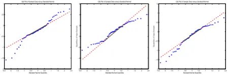
QQ plot as shown in figure 1: From figure one, the three
−2.5 −2 −1.5 −1 −0.5 0 0.5 1 1.5 2 2.5 −2
−1.5 −1 −0.5 0 0.5 1
Standard Normal Quantiles
Quantiles of Input Sample
QQ Plot of Sample Data versus Standard Normal
−2.5 −2 −1.5 −1 −0.5 0 0.5 1 1.5 2 2.5 −6
−4 −2 0 2 4 6
Standard Normal Quantiles
Quantiles of Input Sample
QQ Plot of Sample Data versus Standard Normal
−2.5 −2 −1.5 −1 −0.5 0 0.5 1 1.5 2 2.5 −2
−1.5 −1 −0.5 0 0.5 1 1.5
Standard Normal Quantiles
Quantiles of Input Sample
[image:4.595.319.545.447.521.2]QQ Plot of Sample Data versus Standard Normal
Figure 1: QQ plot of gene expression random variables
subfigures show that some distributions of gene are belong to the ”heavy tail” family, ”light tail” family and ”skewed left” family. From which we could see that the distributions of the gene expression profile random variables are typically non-gaussian, thus,based on central limited theorem, we can get the conclusion that the distributions of the independent also be non-gaussian.
Analysis of the Unmixing Matrix W: We applied ICA
to reduce the dimensionality of the matrixX from 3,894
to 5 ,8 and 12 independent regulator factor components
respectively.Given this p×N matrix X. When we
as-sume there are5independent sources,by the ICA generative
wi (1≤i≤5) one of the rows in the unmixing matrixW
as shown in figure 2.
0 500 1000 1500 2000 2500 3000 3500 4000 −0.02
[image:5.595.60.285.107.196.2]−0.015 −0.01 −0.005 0 0.005 0.01 0.015 0.02
Figure 2: distributions of one row of unmixing matrixW
Becauseyi = wTiX, every estimated regulatory factor
yi is a linear combination of the observed data X, where
wirepresents the contribution of every genes to the
regula-tory factors. From figure 2, we can see that only a coher-ent group of genes ”governing” an independcoher-ent regulatory source. Between the two lines which includes 95% genes have contributes to the independent source less than 0.05. while only 5% genes have relative larger domination.
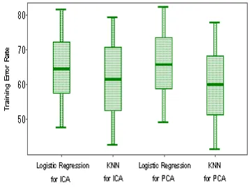
Comparison with PCA for multiclasses classifica-tion:For multiclass classification problem, we use two
clas-sifiers: logistic regression(represents parametric method) and k-nearest neighbor(represents nonparametric method). We use 2/3 of the original data as training cases and the other 1/3 as testing data, because there’re altogether 8 classes and only about 4 training cases for one classes, the classification error is very high, the box plot of these two classifiers based on dimensionality reduction on ICA and PCA are given in figure 3 respectively:
Figure 3: comparision with PCA and ICA for logistic re-gression and kNN classifier
From figure 3, we can see that the performance of ICA based method is better than PCA based method for logistic regression, but a little weaker for k-NN classifier. From the whole point, ICA is a promising method for dimensionality reduction.
5. Conclusion and Future Work
We have proposed an ICA based dimensionality reduction method in this paper, which could be viewed as an exten-sion for PCA based method. Our method could be used to find latent ”regulatory factors” which are statistically inde-pendent between each other, by utilizing our method on the real world dataset, we show that ICA based dimensionality reduction method is promising.
Because our current ICA model is a linear generative model which is based on the assumption that the interac-tions between different regulatory factors are linear, in fact, some of these processes could be unlinear. How to develop an interesting nonlinear ICA model maybe an interesting issue to give some further investigation, thus becomes our future work.
Acknowledgments
The authors would like to thank the referees for reviewing this paper, Han is supported by the graduate fellowship from Department of Computer Science of University of Toronto.
References
[1] Schena, M., Shalon,D. Davis, R.W. and Brown,P.O.
Quantitative monitoring of gene expression patterns with a complementary DNA microarray, Science,vol
270, pp 467-470. 1995
[2] Lockhart,D., Dong,H.,etc.Expression monitoring by
hy-drization to high density of oligonucleotide arrays.,
Nat.Biotechnol, 14, pp.1675-1680,1996
[3] Trevor Hastie, Robert Tibshirani, Jerome Friedman The
elements of statistical learning- Data ming, inference and prediction, Springer 2001.
[4] Althauser, R. P.Multicollinearity and non-additive
re-gression models.,In H. Blaock(ed) Causal models in the
social sciences pp. 453-472. 1971
[5] Mallat,S.G. A wavelet tour of signal
process-ingAcademic, San Diego,2nd 1999
[6] Liebermeister,W. linear modes of gene expression
de-termined by independent component analysis,
Bioinfor-matics 18. pp.51-60,2002
[7] V.S.Cherkassky, I.F.Mulier learning from data,chapter 5. John Wiley & sons,1998
[8] Hyvarinen A. a survey of indepenent component
[image:5.595.87.266.464.600.2][9] Troyanskaya, O., Cantor,M. missing value
estima-tion methods for DNA microarrays, Bioinformatics,17,
pp.520-525,2001
[10] Hyvarinen, A. and Oja,E. Indepdent component
analysi: algorithm and applicatins, Neural networks
13, pp.411-430 2000
[11] Alter O, Brown PO, Botstein D. singular value
decom-position for genome-wide expression data processing and modeling, Pro Natl Acad Sci USA 97,
pp10101-10106 2000
[12] Chippetta,P., Roubaud, M. and Torresani,B. blind
source seperation and the analysis of microarray data,
Proc of JOBIM’02 pp131-136, St Malo 2002
[13] Su-In Lee, Serafim Batzoglou Application of
indepen-dent compoenent analysis to microarrays, Genome
Bi-ology Vol4, R76, 2003
[14] Ross,D.T., Scherf,U.,etc Systematic variation in gene
expression patterns in human cancer cell lines, Nature