2018 International Conference on Modeling, Simulation and Analysis (ICMSA 2018) ISBN: 978-1-60595-544-5
Fluid Simulation and Optimization of a Vehicle's
Outflow Field Based on Fluent
Shu-hua LIAO, Jiong LI
*and Run-ming LU
Guangxi University of Science and Technology, Liuzhou, China 545000
*Corresponding author
Keywords: Outflow field, CFD, Numerical analysis, Visualization.
Abstract. The automobile outflow field directly affects the vehicle's economy, power, operating stability and noise level. CFD fluent software is used to analyze the automobile outflow field and optimize the model. Numerical simulation has become a powerful tool for automobile styling design and analysis and evaluation, and the visualization of its simulation data and results will be of great theoretical and practical significance to the analysis of automobile outflow field.
Introduction
With the rapid development of automobiles in China, the closer the relationship between automobile products and people's life, people put forward higher demands on the performance of automobile, especially the power and economy. In order to improve the speed and save fuel consumption, it is necessary to reduce the vehicle resistance, which is to study the influence of various external shapes on air flow and aerodynamic force. The results show that the aerodynamic resistance becomes the main component of the driving resistance when the vehicle speed reaches a certain numerical value, so how to improve and improve the aerodynamic characteristics of the vehicle is of great significance [1].
The prediction of aerodynamic performance of models if the traditional wind tunnel research method is used, it is necessary to prepare the real car or model, the cost is high, the period is long, the details of the three-dimensional flow field in various states are very difficult to observe in the experiment, which makes the experimental research very limited. Using CFD simulation, we can overcome all kinds of short plates in traditional way, save a lot of time and experiment funds, and can simulate and optimize in the prophase of development, so as to improve the vehicle
aerodynamic performance [2, 3].
Research Theory
All flow and heat transfer processes are subject to three basic equations, and their most concern is the mathematical expression of these conservation laws--partial differential equations, usually called control equations [4].
Continuity Equation
The expression of conservation of mass Law: the increment of fluid mass in a unit time is equal to the net mass of the micro-body at the same time interval, and the following continuity equations can be obtained:
(1)
Momentum Equation
the external force and the inertia force of the fluid micro-element, and the equations of motion deduced from the momentum conservation are:
(2)
Energy Equation
The energy equation reflects the basic properties of energy conservation during fluid flow. For the application of energy conservation law in the microelement in the fluid, the increase rate of the mechanical energy in the microelement is equal to the net heat flux entering the microelement and the work done by the volume force and the surface force on the microelement. The law is actually the first law of thermodynamics, and the energy conservation equation with temperature T as the variable is:
(3)
Turbulence Control Equation
Turbulence is a very common flow type in nature, and the k-ε equation model is the most widely used turbulence model. The turbulent viscosity in the model is expressed as the element flow energy (k) and the turbulent dissipation rate (ε) 2 variables, all of which include convection and diffusion. The form of two equations is as follows.
k equation:
(4) ε equation:
(5)
Value Distribution of Body Surface
In order to establish the expression of the wall function, the dimensionless parameters of velocity
and distance are introduced and , and the expressions are as follows:
(6)
(7)
In order to apply the wall equation effectively, the value cannot be too small, otherwise the
boundary layer includes only laminar boundary layer. At the same time, the value can not be
too large, otherwise the flow characteristics of the boundary may be inconsistent with the description of the wall equation. In engineering, the general requirements of 30< <300, for low
Reynolds number model, requires <2.
Geometric Model Establishment and Grid Division
hardware condition, the real car model is simplified reasonably: headlight, rearview mirror, door handle sag, car antenna and tires, etc., to replace the real concave and convex shape of the bottom of the car with the flat face. These changes in the overall characteristics of the convection field do not
have much impact, but can greatly improve the economic performance of the calculation [1, 5].
At present, the main grid-dividing techniques used in practice are structured grid technology and
unstructured grid technology [6]. In order to reduce the computational load and shorten the
calculation period, the computational field is minimized without affecting the analysis of the flow
field, so as to approximate the flow without interference [7]. Figure 1 is a 3d simulation diagram, the
front three times conductor, five times after car conductor, 6 times the car roof surface is high, one is four times the width, so the simulation of model calculation area as follows: 9 x 4 x 6 h w l (43066 mm * 12320 mm * 12320 mm). Figure 2 is the longitudinal symmetrical surface grid of the body. In ICEM, the car model is divided into unstructured grids, and a reasonable boundary layer is adopted for the car wall surface [8].
Figure 1. 3d simulation diagram of automobile. Figure 2. Body longitudinal symmetrical surface mesh.
Setting of Boundary Conditions
Because the Realizable k-ε turbulence model combines the advantages of Standard k-ε and RNG k-ε models, considering the rotation of airflow and curvature of the surface of the object, the application of the model is very extensive. For example, the rotational uniform shear flow, including free flow of jet and mixed flow, flow in the pipe, boundary layer flow, and separation flow, etc. The convergence speed is much faster than the RNG k-ε turbulence model, and the
calculation results are high. Therefore, the Realizable k-ε model solution is selected in this paper [9].
The boundary condition is the necessary condition that the numerical simulation equation has the definite solution, for the air in the automobile outflow field, because the test speed of the automobile is generally around 35m/s, its Mach number is <0.2, the air density in the airflow is almost unchanged, so the compressibility of the air in the automobile outflow field is not considered
[1]
. That is, the air in the outflow field of an automobile is an incompressible fluid in the numerical simulation of the three-dimensional flow of the automobile outflow field; it is generally believed that the flow field of the physical model is constant, constant temperature and viscous incompressible turbulence.
Main boundary conditions:
Inlet boundary: Airflow Velocity u=30m/s, the turbulent energy coefficient k and viscous dissipation rate ε for inlet boundary are calculated by empirical formula: k=0.032; ε=0.0023.
Export boundary: The pressure is 0 relative to atmospheric pressure, the remaining variable component gradient is 0.
Ground boundary: The vehicle travels on the ground to move the wall boundary, eliminates the surface boundary layer the influence, u=30m/s.
Fixed wall surface (Vehicle model outer surface) boundary: in order to meet the fixed wall without slip conditions, the wall boundary velocity of 0.
Simulation Results and Analysis
Through the post processing of fluent, the results of the outflow field calculation can be visualized. From figure 3 the pressure cloud of the automobile outflow field and figure 4 pressure amplification cloud diagram can be seen that, due to the flow speed and the front car body meet, leading to the front pressure, front part, hood, near the border with windscreen and rear windshield and suitcase cover basic for positive pressure near the border area, air flow in the front is hampered by a large, will be near the border are to form a strong vortex. Due to the flow rate is greater than the velocity of the bottom of the car roof, so there is an obvious negative pressure zone, in the body at the top of the car and car at the top of the pressure difference is formed at the bottom of the lift, thereby affect the adhesion performance.
[image:4.595.186.523.520.631.2]
Figure 3. The pressure cloud of the automobile outflow field Figure 4. Pressure amplification cloud diagram.
Figure 5 the velocity vector distribution diagram of the body symmetry plane, figure 6 is the tail velocity vector amplification diagram. Can be seen near the body, the air flow is obviously affected by the car, airflow in the front of the car is blocked by the car, this is an important reason for air resistance. The airflow in the front of the car is divided into two parts, most of it flowing up the hood, and partly to the bottom of the car. Some of the air near the ground must be forced to pass between the bottom of the body and the pavement, the flow line in the back of the car does not terminate, but the formation of eddy currents, resulting in resistance, so in the longitudinal direction of the tail, you can clearly see the area near the rear of the car generated a large vortex, where the flow is unusually complex, occurs at a sharp speed pulsation. The increase in airflow from the bottom of the vehicle increases the aerodynamic resistance and the cleanliness of the rear. Therefore, the automobile tail fluid must be optimized to reduce vortex generation, reduce resistance, and ensure the cleanliness of the tail.
Figure 5. Velocity vector distribution diagram Figure 6. Tail velocity vector amplification diagram.
Vehicle Optimization
Aiming at some problems of SUV, a reasonable optimization scheme is proposed to improve it. In the upper end of the car, the spoiler is added to guide the flow of airflow, improve the vortex state of the tail airflow, and achieve the desired target.
Table 1. Comparison of vehicle data before and after optimization.
Before optimization After optimization
Aerodynamic drag coefficient 0.485 0.343
Aerodynamic lift coefficient -0.045 -0.076
Aerodynamic force (N) 782.625 486.324
[image:5.595.183.409.390.638.2]
Figure 7. The optimized post pressure cloud picture. Figure 8. The optimized post pressure amplification cloud.
Figure 7 is the optimized symmetry surface pressure cloud picture and Figure 8 is the optimized post pressure amplification cloud can be seen, due to flow speed and the front meet, airflow encountered the front of a block, so the head of the windward part still present positive pressure zone, which is conducive to the engine forced intake. But through optimization, the maximum of the positive pressure area of the front face of the vehicle is reduced, and the maximum positive pressure value is reduced from the original 602 MPa to 586 MPa, and the negative pressure area of the back of the original roof is reduced.
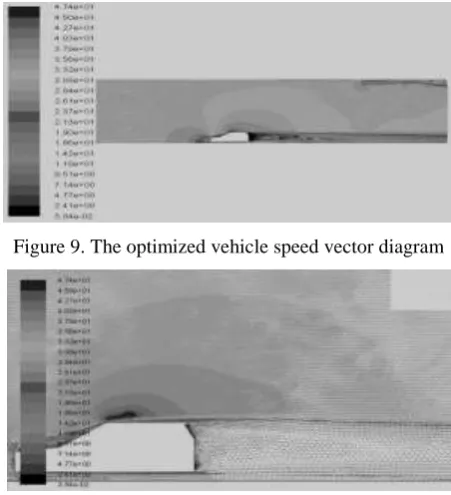
Figure 9. The optimized vehicle speed vector diagram
Figure 10. The optimized body velocity vector amplification diagram
Figure 9 is the optimized vehicle speed vector diagram and figure 10 is the optimized body velocity vector amplification diagram, in the case of the basic flow unchanged, from the figure can be seen in the top of the car, added the tail spoiler on the flow of the weak disturbance, the reversal of the basic disappeared, forming a weaker vortex and dispersed to the rear diffusion, the tail streamline obvious rules flow, Thus, the control of the wake airflow changes gently and reduces the energy dissipation in the wake area. The aerodynamic performance of the vehicle is improved.
Summary
[image:5.595.183.411.392.513.2] [image:5.595.185.416.523.635.2]and can get the pressure cloud picture and the velocity cloud chart of the automobile outflow field, and after understanding the distribution of the airflow, the original model has been optimized. The comparative study on the automobile outflow field of a certain model based on the optimized model shows that the flow field is more fluent, the range of the vehicle tail vortex is reduced, and the airflow change is gentle and the resistance is reduced. According to the simulation results and the actual situation of the automobile outflow field, it is very important to use the CFD method to guide the aerodynamic characteristics of automobiles.
Reference
[1] Limin Fu. Automotive Aerodynamics [M].Beijing: Machinery Industry Press, 1998.
[2] Kataoka T, China H. Numerical Simulation of Road Vehicle Aerodynamics and Effect of Aerodynamic Devices. SAE910597.
[3] Jing Zhao. The Research of Ground Effect in Automotive Wind Tunnel Based on Numerical Simulation [D]. Changchun: Jilin University, 2011.
[4] Zhengqi Gu, Lehua Jiang, Jun Wu, Gang Fang. The Numerical Analysis and Computer Simulation on Automobile Flowfield [J]. Journal of Aerodynamics, 2000.
[5] Hualin Li. The Aerodynamic Simulation and Optimization of the Design for External Flow Field of Automobile Based on FLUENT [D]. Lanzhou Jiaotong University, 2014.
[6] User Guide of Computational Fluid Dynamics Software [EB/OL].STAR-CD version, 2004.
[7] Liping Huang, Yongchang Dai, Chunbo Li, PDM Fast-Implementation Assistance System [J]. Computer Integrated Manufacturing System –CIMS, 2003.
[8] Wenling Gu, Junjie Cui, Characteristics of Car External Flow Field Based on Fluent [J]. Agricultural Equipment and Vehicle engineering, 2014, 52 (3): 55-57, 65.