Fractal video compression

University of Southern Queensland

Faculty of Engineering and Surveying

Fractal Video Compression

A dissertation submitted by

Khalid Kamali

in fulfilment of the requirements of

Courses ENG4111 and ENG4112 Research Project

towards the degree of

Bachelor of Engineering (Computer Systems)

Abstract

With the rapid increase in the use of computers and internet, the demand for higher transmission and better storage is increasing as well. One way to solve this problem is by using compression, in which a small amount of data can represent the much larger amount of original data.

This dissertation describes the different techniques for data (image-video) compression in general and, in particular, the new compression technique called Fractal Image Compression. Fractal image compression is based on self-similarity, where one part of an image is similar to the other part of the same image.

University of Southern Queensland

Faculty of Engineering and Surveying

ENG4111 & ENG4112 Research Project

Limitation of Use

The Council of the University of Southern Queensland, its Faculty of Engineering and Surveying, and the staff of the University of Southern Queensland, do not accept any responsibility for the truth, accuracy or completeness of material contained within or associated with this dissertation.

Persons using all or any part of this material do so at their own risk, and not at the risk of the Council of the University of Southern Queensland, its Faculty of Engineering and Surveying or the staff of the University of Southern Queensland.

This dissertation reports as educational exercise and has no purpose or validity beyond this exercise. The sole purpose of the course pair entitled “Research Project’ is to contribute to the overall education within the student’s chosen degree program. This document, the associated appendices should not be used for any other purpose: if they are so used, it is entirely at the risk of the user.

Prof G Baker

Dean

Certification of Dissertation

I certify that the ideas, designs and experimental work, results, analyses and conclusions set out in this dissertation are entirely my own effort, except where otherwise indicated and acknowledged.

I further certify that the work is original and has not been previously submitted for assessment in any other course of institutions, except where specifically stated.

Khalid Kamali

0031137033

Signature

Acknowledgments

This project would not have been possible without the assistance and support of many people. I would like to take this opportunity to thank my supervisor, Dr John Leis, my family and friends for their encouragement and guidance throughout the year.

Khalid Kamali

University of Southern Queensland

Table of Contents

Abstract... i

Certification of Dissertation... iii

Acknowledgments... iv

Chapter 1... 1

Introduction... 1

1.1 Project Objectives ... 2

1.2 Image Quality... 2

1.3 Test Images ... 3

1.4 Outline of the Dissertation ... 4

Chapter 2... 5

Image and Video Compression... 5

2.1 Image Compression Methods ... 5

2.1.1 Huffman Coding ... 5

2.1.2 Arithmetic Coding ... 7

2.1.3 Vector Quantization ... 8

2.1.4 DCT (Discrete Cosine Transform)... 9

2.1.5 BTC (Block Truncated Coding)... 10

2.1.6 JPEG/JPG (Joint Photographic Experts Group) ... 11

2.2 Video Compression... 13

2.2.1 Frame Differencing... 14

2.2.2 Motion-compensation Prediction... 14

2.3 Chapter Summary ... 15

Chapter 3... 16

Fractal Image Compression ... 16

3.1 History of Fractal Image Compression ... 16

3.2 How Does Fractal Image Compression Work? ... 16

3.3 The Contractive Mapping Fixed-Point Theorem... 18

3.4 Fractal in Image Compression ... 18

3.5 Fractal Compression and the Self-similarity... 19

3.6 Affine Transformation ... 20

3.7 Iterated Function System ... 21

3.8 Fractal Image Compression algorithm... 22

3.8.1 Encoding ... 22

3.8.2 Decoding... 23

3.9 Chapter Summary ... 25

Chapter 4... 26

Performance of Fractal Image Compression... 26

4.1 Compression Rate ... 26

4.2 Image Quality... 29

4.3 Fractal Vs JPEG/JPG and BTC... 32

4.4 Chapter Summary ... 36

Fractal Color Image Compression ... 37

5.2 Red, Green and Blue ... 37

5.3 YIQ and YUV ... 40

5.4 Chapter Summary ... 44

Chapter 6... 45

Different Partitioning Methods ... 45

6.2 Quadtree Partitioning ... 45

6.3 Horizontal-Vertical Partitioning ... 46

6.4 Triangular Partitioning... 47

6.5 Chapter Summary ... 48

Chapter 7... 49

Faster Encoding ... 49

Chapter 8... 51

Fractal Video Compression... 51

Chapter 9... 55

Conclusions and Further Work ... 55

9.1 Achievement of Objectives... 55

9.2 Further Work... 56

References... 57

List of Tables Table 2.1: The probability for each character... 6

Table 2.2: The probability and range for each character in the arithmetic coding. ... 7

Table 2.3: The encoding steps in arithmetic coding. ... 8

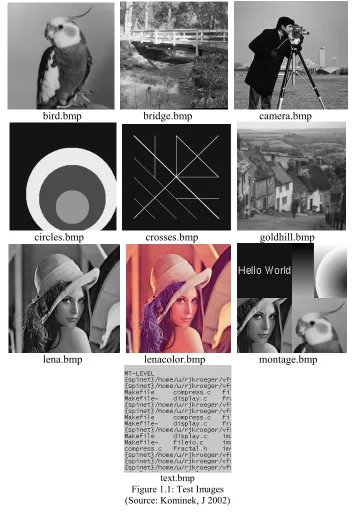
List of Figures Figure 1.1: Test Images... 3

Figure 2.1: Huffman code construction. ... 6

Figure 2.2: Block diagram of Vector Quantization image coder... 9

Figure 2.3: DCT-based coding system... 10

Figure 2.4: DCT basis... 10

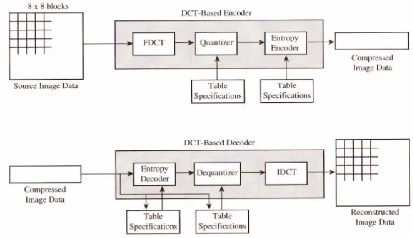
Figure 2.5: The basic JPEG/JPG Encoder and Decoder ... 12

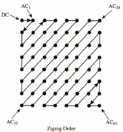
Figure 2.6: Zigzag Coefficient Ordering ... 13

Figure 3.1: A copy machine... 17

Figure 3.2: first three copies generated by the copy machine... 17

Figure 3.3: The output of the copy machine after n iterations... 17

Figure 3.4: Lena image showing ranges and domains... 19

Figure 3.5: Showing the original Lena image and the Decoded Images after 1, 2, 4 and 8 iterations... 24

Figure 3.6: The Convergence towards the fixed point for Lena image ... 25

Figure 4.1: Decoded Lena image with error image using 4x4, 8x8 and 16x16 range blocks ... 28

Figure 4.2: The convergence of Lena image using 4x4, 8x8 and 16x16 range blocks... 29

Figure 4.3: Quality of the decoded test images after 12 iterations ... 30

Figure 4.5: Lena original and decoded zoomed in... 32

Figure 4.6: PSNR values for the decoded text images using the three techniques with an approximated compression rates for the three techniques ... 33

Figure 4.7: PSNR values for decompressed Lena image using different levels of compression ratio for both fractal-based compression and JPEG/JPG... 34

Figure 4.8: Lena image decompressed using fractal-based compression and JPEG/JPG with different compression ratios... 35

Figure 5.1: color palette as a lookup table to produce a pixel ... 38

Figure 5.2: The Red, Green and Blue components of Lena color image... 39

Figure 5.3: The convergence of the Red, Green and Blue images using the RGB components ... 41

Figure 5.4: The convergence of the Red, Green and Blue images using the YIQ components ... 42

Figure 5.5: The convergence of the Red, Green and Blue images using the YUV components ... 42

Figure 5.6: (a) Original Lena color image. (b) Decompressed Lena color image using the RGB components. (c) Decompressed Lena color image using the YIQ components. (d) Decompressed Lena color image using the YUV components ... 43

Figure 6.1: Quadtree Partition... 46

Figure 6.2: Partitioning Lena image using H-V partition ... 47

Figure 6.3: Partitioning Lena image using Triangular partition ... 48

Figure 7.1: Lena image with domain blocks used in black... 50

Figure 8.1: Video clip frames ... 52

Figure 8.2: Range cubes and domain cube in a GOF ... 54

Appendices Appendix A... 61

Chapter 1

Introduction

Day by day, the demands for higher and faster technologies are rapidly increasing for everyone. Although the technologies available now are considered more advanced than 30-40 years ago, people are still looking for improvements and enhancements. In the last twenty years, computers have been developed and their price has reached a level of acceptance where almost anyone can buy one. Nowadays, before purchasing computers, customers are concerned about two things: (1) the speed of the CPU; and (2) the storage and memory capacity.

1.1 Project

Objectives

The main objectives of this project are:

1- To investigate and have a general idea of several compression techniques. 2- To investigate and have a good understanding of fractal image compression. 3- To use MATLAB to implement fractal image compression for both gray-scale

images and color images.

4- To discuss methods of improving the performance of fractal image compression. 5- To compare fractal image compression and some other compression techniques. 6- To investigate and use MATLAB to implement fractal video compression.

1.2 Image Quality

In this project PSNR (Peak Signal to Noise Ratio) is used to compute the quality of the reconstructed image compared with the original image by measuring the differences between the two images; the formula used to compute the PSNR is [8].

PSNR = 20 log₁₀

(

)

where b is the highest pixel value (255) and rms is the root mean square

differences between the two images. PSNR is measured in dB, the highest the PSNR, the better the quality of the reconstructed image. Nevertheless, this is not the only way used to measure the quality of images—there are other ways but PSNR is the most widely used.

1.3 Test Images

Throughout this project, a set of images been used to test the quality and the performance of the fractal image compression and other types of compression. The gray-scale images are of size 256 x 256 and the only color image is of size 512 x 512. Figure 1.1 shows the full set of the test images.

bird.bmp bridge.bmp camera.bmp

circles.bmp crosses.bmp goldhill.bmp

lena.bmp lenacolor.bmp montage.bmp

1.4 Outline of the Dissertation

Chapter 2: Image and Video Compression. This chapter contains a brief description of types of compression and some compression techniques for both images and videos.

Chapter 3: Fractal Image Compression. This chapter gives an overview the history of fractal-based compression, together with some mathematical background and a brief outline of the concept of fractal-based compression.

Chapter 4: Performance of Fractal Image Compression. This chapter shows the performance of fractal image compression for gray-scale images in terms of quality and compression rates, together with a comparison between fractal-based compression and some other compression techniques.

Chapter 5: Fractal Color Image Compression. This chapter contains the methods used to encode a color image using a fractal-based compression, and looks at the performance of the decompression using different coordinate systems of the color image.

Chapter 6: Different Partitioning Methods. This chapter contains different partitioning approaches in fractal image compression, and details the advantages and disadvantages of using each approach.

Chapter 7: Faster Encoding. This chapter contains different procedures adopted to reduce encoding time in the case of fractal image compression.

Chapter 2

Image and Video Compression

2.1 Image Compression Methods

Primarily, there are two types of image compression: one is called lossless and the other

is lossy. Lossless method describes when the decompressed image is exactly as the

original image and there is no loss of information. On the other hand, lossy has some information loss after decompressing the image, however, this loss of data is considered negligible (if the loss of data is acceptable), since the difference between the reconstructed image and the original image is not large and remains relatively unchanged.

This chapter looks at several compression techniques with a brief description of each one. Some of those compression techniques belong to lossless compression and others to lossy compression.

2.1.1 Huffman Coding

One of the oldest coding techniques is Huffman coding; it was first introduced by David Huffman in 1952.

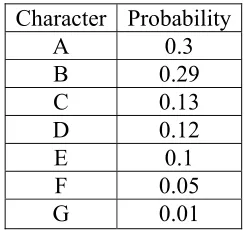
For example, let’s take the encoding of this page that you are reading, then first to be found is the probability for each character in this page; to make the example more simple, let’s say this page only contains seven characters—each has a probability of what is shown in the table below:

Character Probability A 0.3 B 0.29 C 0.13 D 0.12 E 0.1 F 0.05 G 0.01

Table 2.1: The probability for each character.

Now, based on the probability of each character, a binary tree is formed, starting with two child nodes which represent the two characters with the lowest probability. Taking these two from the list we add the next lowest probability character to the tree, continuing to do so until we reach to the root of the tree. After that we label one side of the tree with 0s and the other with 1s (it does not matter which side is which).

1 A 1 1

B 0.7 0 1

C 0.41 0 1

D 0.28 0 1

E 0.16 0 1

F 0.06 0

0 G

2.1.2 Arithmetic Coding

Arithmetic coding is a lossless type of compression, and it is very similar to Huffman coding except for that it does not produce a single code for each symbol but, rather, it produces a specific codeword for the whole message. The codeword is in the form of a float point number between 0 and 1.

The idea in arithmetic coding is to generate a probability table in the same way as the Huffman coding, and then to assign each symbol with a range between 0 and 1. The symbols with higher probabilities will be assigned to wider ranges and the symbols with lower probabilities be assigned to smaller ranges [5, 6, 20, 22].

For illustration, we will encode the word ‘TARA’. First, we form the following table showing the probability and range for each character:

Character Probability Range

A 0.5 0.0-0.5

R 0.25 0.5-0.75

T 0.25 0.75-1.0

Table 2.2: The probability and range for each character in the arithmetic coding.

Then we start coding using the following algorithm [6]:

LOW = 0.0

HIGH = 1.0

WHILE not end of input stream

Get next CHARACTER

RANGE = HIGH – LOW

HIGH = LOW + RANGE * high range

Low = LOW + RANGE * low range

END While

The following table (Table 2.3) shows how the range, high and low, changes as each character is processed:

T Range=1 Low=0.75 High=1

A Range=0.25 Low=0.75 High=0.875

R Range=0.125 Low=0.8125 High=0.84375

A Range=0.03125 Low=0.8125 High=0.828125

Table 2.3: The encoding steps in arithmetic coding.

Final output of the encoding will be equal to 0.815.

The decoding process is simply the inverse of the encoding.

2.1.3 Vector Quantization

Vector Quantization (VQ) follows the lossy type of data compression. In VQ the encoding process is quite complex, however, this complexity makes the decoding process very fast.

In the process of image compression using vector quantization, first the image is divided into smaller sections called target vectors. Then, each target vector will be encoded as a

code vector which is introduced by matching the target vector with the codeword from

the codebook (finding the minimum distortion). The codebook is formed from a collection of many representative images, therefore, it should contain all the possible representations of the target vectors. By transmitting only the index of each best matching codeword it is possible to obtain a good compression ratio because each section of the image will be only represented with an 8-bit codeword index. In the decoding process, the decoder should have the same codebook as the encoder, and then simply by using the saved codeword index and a look-up table the original image is reproduced [4, 8].

Figure 2.2: Block diagram of Vector Quantization image coder (Source: Bhaskaran-et-al, V 1995)

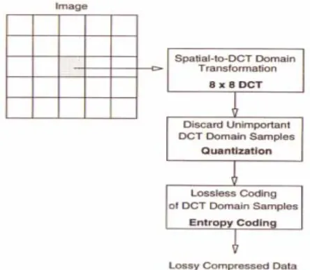
2.1.4 DCT (Discrete Cosine Transform)

Most of the image and video compression standards such as JPEG and MPEG are based on the DCT coding. DCT compression is another type of lossy compression.

Discrete cosine transform is very much related to the well-known FFT (Fast Fourier Transform), in as much as they both change the data from its current domain to frequency domain, however, DCT only deals with real numbers—unlike FFT which suffers from complex multiplications.

Figure 2.3: DCT-based coding system (Source: Bhaskaran-et-al, 1995)

Figure 2.4: DCT basis (Source: Barnley, MF 1993)

2.1.5 BTC (Block Truncated Coding)

described as faster and more efficient than vector quantization. This is because in BTC the conversion of the blocks into simpler forms will preserve some statistics of the original blocks—unlike vector quantization which relies on the approximations of the blocks in the codebook.

In this method the image is divided into blocks of pixels each with the size of n x n

(usually 4 x 4), then finding the mean or the average of the block to be used as a threshold. Pixels are then classified to high or low, depending on that threshold. For the reconstruction process of the block we will use two values, a and b—these two values

will be close enough to the original values.

a = xm - σ (q / (n – q))

2 /

1 _(2.1)

b = xm + σ ((n – q) / q)

2 / 1

(2.2)

where: x_m is the mean, σ is the variance, q is number of pixels greater than mean and n

is the number of pixels in the block [5].

2.1.6 JPEG/JPG (Joint Photographic Experts Group)

Nowadays, JPEG/JPG is the most widely recognized compression; JPEG/JPG is a lossy type of compression developed by the Joint Photographic Experts Group and was first

accepted as an international standard in 1992.

JPEG/JPG is based on DCT, and the encoding and the decoding of it consists of several steps that each contributes to compression. The first step of the encoding process is partitioning the image into blocks of 8 x 8, then for each block the FDCT (Forward

Discrete Cosine Transform) is computed. The 64 DCT coefficients are then scalar

Encoder” which is used to send out the coefficients codes by using either Huffman

Coding or Arithmetic Coding. The decoding, as illustrated in Figure 2.6, is simply the inverse process of the encoding [10, 15, 18, 22].

Figure 2.6: Zigzag Coefficient Ordering (Source: Gibson-et-al, 1998)

2.2 Video Compression

Video is a number of images in sequence; therefore, the same way we compress images can be applied on the video by compressing each frame of the video separately (this is called intra-frame coding). Though this technique looks very simple, it is impractical

because it requires a very large memory space to store data. The best way to achieve a better compression is in taking advantage of the similarities between the video frames (this advantage is also used in fractal video compression and discussed in chapter 8 of this dissertation). There are two main functions used in video coding [24]:

1- Prediction: create a prediction of the current frame based on one or more

previously transmitted frames.

2- Compensation: subtract the prediction from the current frame to produce a

2.2.1 Frame Differencing

The idea of frame differencing in video coding is to produce a residual frame by subtracting the previous frame from the current frame; the residual frame will then be a form of zero data, with light and dark areas (light indicates positive residual data and the dark indicates negative residual data). Nevertheless, there will be more portions in the residual frame with zero data than the light and dark; this is due to the similarity between the frames (most of the pixels in the previous frame will be equal to the pixels in the current frame). Therefore, since more of the residual frame is zero data, then the compression efficiency will be further improved if we compress the residual frame instead of the current frame. Frame differencing method in video coding faces a major problem which is best illustrated by the following example. In the encoding and the decoding process for the first frame, there will be no prediction, but the problem starts with the second frame when the encoder uses the first frame as the prediction and encodes the resulting residual frame. Here, we are dealing with a lossy type compression; the decoded first frame is not exactly the same as the input frame, which leads to a small error in the prediction of the second frame at the decoder. This error will increase as we continue with the following frames and the result will be low quality in the decoded video sequence.

There is one way in which this problem can be solved; the idea is that when we encode the first frame we decoded immediately and use the decoded frame to form the prediction for the second frame [24].

2.2.2 Motion-compensation Prediction

compression may not be significant. This is due to the movement in the video scene. So, in this type of frames we use another method of prediction called Motion-compensation Prediction; where the achievement of better prediction is by estimating the movement and compensating for it. Motion-compensation is similar to Frame differencing with two extra steps [4, 24]:

1- Motion estimation: comparing a region in the current frame with the neighboring

regions of the previous decoded frame and finding the best match.

2- Motion Compensation: Subtracting the matching region from the current region.

The encoder will send the location of the best match to the decoder to perform the same motion compensation operation in the process of decoding the current frame.

The residual frame in motion-compensation contains less data compared with frame differencing (higher compression); however, motion-compensation is very computationally intensive.

2.3 Chapter Summary

Image and video compression is very necessary to reduce the capacity required for storing data and also to shorten the time required for sending data. Compression of image and video is divided into two categories—lossy and lossless. With lossless compression we cannot achieve high rates of compression but the decoded image or video will be exactly same as the input; on the other hand, with lossy type we obtain high compression rates but lose some data. However that loss of data is not significant since human visual systems cannot detect it.

Chapter 3

Fractal Image Compression

3.1 History of Fractal Image Compression

The idea of fractals is not new—it goes back to the beginning of the last century. However, no one really understood or paid attention to the importance of fractals and its geometry until 1977 when Benoit Mandelbrot published his book The Fractal Geometry

of Nature. Mandelbrot, in his book, tried to show the existence of fractals in nature—like

clouds, mountains and trees. However, he did not think of fractals as a method for compression. Michael Barnsley was the first person to use the idea of fractals in image compression. It has been claimed that fractal coding may reach compression ratios up to 10000:1—which sounds like a very impressive rate of compression. However, it doesn’t have a standard because it suffers from such problems as very expensive encoding time and, therefore, it is still under discussion and being studied.

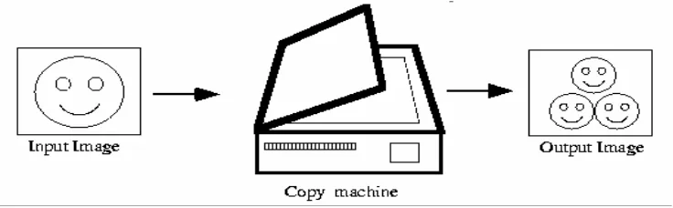
3.2 How Does Fractal Image Compression Work?

Figure 3.1: A copy machine. (Source: Fisher, Y 1995)

Now if we feed back the output as an input and repeat the same process for two more times, we will end up with the shape showing in Figure 3.2 below:

initial image first copy second copy third copy

Figure 3.2: first three copies generated by the copy machine. (Source: Fisher, Y 1995)

If we continue doing the same thing again and again for a number of times (n iterations),

at some stage we will reach the following (see Figure 3.3 below):

Figure 3.3: The output of the copy machine after n iterations. (Source: Fisher, Y 1995)

and the orientation of the copies will decide the final shape of the final image. In other words, the final image will be determined by the way the input image is transformed. This transformation of the input image must be contractive or, in other words, the

transformation of two points in the input image must bring the points closer at the output [8].

3.3 The Contractive Mapping Fixed-Point Theorem

The contractive mapping fixed-point theorem state: A transformation f :X → X on a

metric space (X, d) is called contractive if there is a constant 0≤s<1 such that [1, 2, 8,

16]:

) , ( . )) ( ), (

(f x f y sd x y

d ≤ ∀ x,y∈X

(where s = contractivity factor)

And a point a∈X is called a fixed point of the transformation f if f (a) =a.

In other words, the convergence to the fixed point or the attractor depends on the contractivity of the mappings. We say a map is contractive when it brings points closer to each other. For example, let’s consider the map f(x)=x/2—this map is contractive

because if we take any initial value to be x, then by computing f(x),f(f(x)), f3(x),…, the

convergence will be toward the fixed point which is 0.

3.4 Fractal in Image Compression

similar to larger parts of the same image called domain blocks. Fractal image compression is of the lossy type, since the decompressed image is not the same as the original image.

3.5 Fractal Compression and the Self-similarity

The self-similarity in images is unlike the self-similarity in fractals—in fractals self-similarity is almost perfect or exactly the same. However, in real images, such as the images of people, trees, clouds and nature, there are different types of self-similarity, where one part of the image is similar to the other but not the entire image. Even the self-similarity may not be identical. Figure 3.4 below shows the self-similarity of two parts of the image with different scales; the small squares represent the ranges and the large squares represent the domains:

3.6 Affine Transformation

The general form of the Affine Transformation in R2 is [1, 9, 33]:

w

( )

⎠ ⎞ ⎜⎜ ⎝ ⎛ 2 1 x x = _⎜⎜ ⎝ ⎛ c a ⎟⎟ ⎠ ⎞ d b ⎟⎟ ⎠ ⎞ ⎜⎜ ⎝ ⎛ 2 1 x x + _⎟⎟ ⎠ ⎞ ⎜⎜ ⎝ ⎛ f e (3.1)

The matrix _⎜⎜ ⎝ ⎛ c a ⎟⎟ ⎠ ⎞ d b

is equal to _⎜⎜ ⎝ ⎛ 1 1 1 1 sin cos θ θ r r _⎟⎟ ⎠ ⎞ − 2 2 2 2 cos sin θ θ r r

So, equation (1) can be written as:

w

( )

⎠ ⎞ ⎜⎜ ⎝ ⎛ 2 1 x x = _⎜⎜ ⎝ ⎛ 1 1 1 1 sin cos θ θ r r ⎟⎟ ⎠ ⎞ − 2 2 2 2 cos sin θ θ r r ⎟⎟ ⎠ ⎞ ⎜⎜ ⎝ ⎛ 2 1 x x + _⎟⎟ ⎠ ⎞ ⎜⎜ ⎝ ⎛ f e (3.2)

Affine transformations are able to skew, stretch, scale, rotate and translate an input image. There are thousands or millions of transformations, therefore, to make the compression process easier (reducing the domain pool, decreasing the searching time); Jacquin (Arnaud Jacquin, one of Barnsley’s students) suggested having the range and domain blocks to be always square and the domain size to be twice the size of the range. Also, he suggested having only eight transformations for the domain blocks:

1. Rotation by 0. 2. Rotation by 90. 3. Rotation by 180. 4. Rotation by 270.

8. Flip about reverse diagonal.

In dealing with gray scale images, intensity of pixels should be treated as a third spatial dimension, thus the affine transformation for the gray scale images will become:

w

( )

⎟ ⎟ ⎟ ⎠ ⎞ ⎜ ⎜ ⎜ ⎝ ⎛ 3 2 1 x x x = ⎜ ⎜ ⎜ ⎝ ⎛ 0 c a 0 d b ⎟ ⎟ ⎟ ⎠ ⎞ s 0 0 ⎟ ⎟ ⎟ ⎠ ⎞ ⎜ ⎜ ⎜ ⎝ ⎛ 3 2 1 x x x + ⎟ ⎟ ⎟ ⎠ ⎞ ⎜ ⎜ ⎜ ⎝ ⎛ o f e (3.3)

where s represents the contrast (luminance) and o represents the offset to the pixel

contrast which is the brightness of the transformation.

3.7 Iterated Function System

Iterated Function System (IFS) was first introduced by John Hutchinson in 1981 and developed by Michael Barnsley in 1988. IFS play the main rule in fractal image compression. From the word ‘iteration’ we know that it is something repeating. IFS takes the output of the first iteration as the input to the second iteration and continues doing that until it reaches the last iteration. Fractal image compression is based on Iterated Function System; the idea of IFS is to have a finite set of contraction mappings in which they are written as affine transformations. By applying IFS to a seed image (which is the same size of the original image) and provided the mapping is contractive (reducing the distance and bringing the points together), ultimately the final result is the attractor

image or the fixed point. Iterated function system is not really practical in terms of it

image into non-overlapping blocks of ranges and then apply IFS on each block of ranges [22].

3.8 Fractal Image Compression algorithm

3.8.1 Encoding

The encoding process of fractal image compression is not complicated, but very time consuming. In this project, the MATLAB codes written for this project (Appendix B) deal with both gray-scaled and color images, and the algorithm used is the classical way where the range and domain are square (later in the dissertation we will look at different types of partitioning). We can sum the encoding process in the following steps:

1- Read an image (the images used in this project are of the square size).

2- Partition the image into non-overlapped blocks of ranges of square sizes covering the whole image and non-overlapped blocks of domains (and we can take overlapped blocks), twice the size of range block.

Note: Using non-overlapped domain blocks is much better since we will have a larger domain pool to be compared with each of the range blocks for best matching. However, it will take a very long time compared with non-overlapping blocks of domain. Later in the dissertation it will be demonstrated that even with using non-overlapped domain blocks the resulting decoded images are acceptable in terms of quality.

3- Rescale the domain blocks (to the same size of range blocks) and find the eight possible transformations for each block.

4- Compare each range block with whole domain blocks to find best match. 5- Save the following coefficients:

• The location of the domain. • Best transformation.

• Offset.

6- Continue doing the same for the rest of the range blocks until the last one is reached.

3.8.2 Decoding

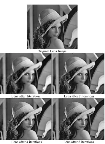
The decoding in fractal compression is much faster compared with the encoding; here the time depends on the number of iterations, however, we will see that only a few iterations (usually after 4-8 iterations) are required to reach the fixed point or the attractor. In this project, we will see that only after 4 iterations we are getting to the fixed point, as illustrated in Figure 3.5 and Figure 3.6.

The following are the steps used in the decompressing process of fractal-based compression:

1- Load the saved coefficients.

2- Create memory buffers for the range and domain screens. 3- Apply the Affine coefficients on the domain screen. 4- Copy the content of the domain screen to the range screen.

5- Take the output of first iteration (range screen) to be the input of the next iteration.

Original Lena Image

Lena after 1iteration Lena after 2 iterations

Lena after 4 iterations Lena after 8 iterations

Figure 3.6: The Convergence towards the fixed point for Lena image.

3.9 Chapter Summary

Fractal image compression is mainly based on the self-similarity within the image; the image is divided into blocks of ranges and domains. The main task in fractal image compression is to find for each range block a corresponding domain block. The search for the best match between the range and domain blocks makes the encoding computationally very expensive, however, the following chapters explore some methods which have been adopted to reduce the searching time.

Chapter 4

Performance of Fractal Image Compression

This chapter focuses on the performance of fractal image compression in terms of compression rate, image quality and comparison with two other compression techniques; BTC (Block Truncated Coding) and JPEG/JPG (Joint Photographic Experts Group). The codes used for fractal image compression were implemented using MATLAB (Appendix B). BTC (Source: Lucey, 1998) and JPEG/JPG (Source: Skiljan, 2005) compression were implemented using MATLAB and irfanview respectively.

4.1 Compression Rate

In fractal image compression the achievement of different levels of compression ratios are dependent on the size of the range blocks. Compression occurs because each block of range is represented by only five values. These values are [33]:

• e & f: Represent the location of the corresponding domain block and each takes 8

bits.

• M: Is the transformation of the domain block and takes 3 bits

• s: Is the contrast and takes 5 bits.

In this project, three different sizes of the range blocks are taken as the following; 4 x 4, 8 x 8 and 16 x 16. The compression ratio is then calculated as follows:

In the case of 4 x 4 range blocks, the compression rate is: 8 + 8 + 3 + 5 + 6 = 30 bits/(4 x 4) pixels (16 bytes) = 1.875/pixel. (≈4.25:1)

In the case 8 x 8 range blocks, the compression rate is: 8 + 8 + 3 + 5 + 6 = 30 bits/(8 x 8) pixels (64 bytes) = 0.46875/pixel. (≈17.00:1)

And in the case of 16 x 16 range blocks, the compression rate is: 8 + 8 + 3 + 5 + 6 = 30 bits/(16x16) pixels (256 bytes)

= 0.117/pixel. (≈68.00:1)

It is important to mention that experiments have shown that it is not necessary to have the same value of s (contrast) used in the encoding to be used in the decoding process;

instead we can use a set of values for s between 0 and 1in the encoding process and use

only a single value or the same set for the decoding process, therefore, it is not necessary to save the s values, which means obtaining a higher compression rate [7].

Lena 4x4 Error Image

Lena 8x8 Error Image

Lena 16x16 Error Image

Figure 4.2: The convergence of Lena image using 4x4, 8x8 and 16x16 range blocks.

4.2 Image Quality

Figure 4.3: Quality of the decoded test images after 12 iterations

Another fact worth reiterating is that the image will not reach the fixed point (the final output image) until after some number of iterations. In this project, the results have shown that at least four iterations are required in order to gain a good output image (reaching the fixed-point). On the other hand, in the case of the text image it does not matter how many iterations are applied, the output image will always be low in quality and unreadable.

Fractal-based compression based on the self-similarity, then the size of the domain pool, also plays a significant role in the quality of the output image. With bigger domain pool and more possible transformations of the domain blocks, each range block will have more chance of finding the best/right corresponding domain block (best match). Consequently, the more the domain block is similar to the range block, the more the quality of the output image increases. 0 5 10 15 20 25 30 35 bird brid ge cam era circ les cro sses goldh ill lena mo

Original text image

Decompressed text image using fractal 4x4

Figure 4.4: Original and Decompressed text image

One other important feature regarding the quality of fractal image compression is

the decoded image will not be blocky and it will contain details at every scale (see Figure 4.5). The decoded process creates an artificial detail which was not presented in the original image. This is due to the iterations in the decoding process; after each iteration the details on the decoded image becomes smoother [5, 8, 16, 22].

Original image Decoded image

Figure 4.5: Lena original and decoded zoomed in. (Source: Lu, N 1997)

4.3 Fractal Vs JPEG/JPG and BTC

In this section there will be a comparison between the fractal-based compression and two other lossy type of compressions: JPEG/JPG (Joint Photographic Experts Group) and BTC (Block Truncated Coding). However, since JPEG/JPG is widely used and one of the most famous around the world, it will be discussed further in this section and contrasted in terms of quality and compression ratios.

0 10 20 30 40 50 60 70 80 bird brid ge cam era circ les crossesgo ldhi ll len a mo ntag e text test images P S NR( d B ) BTC FRACTAL 4x4 JPEG/JPG

Figure 4.6: PSNR values for the decoded text images using the three techniques with an approximated compression rates for the three techniques.

The BTC code used in this project uses 4 x 4 blocks only, with a compression rate of 2 bits per pixel. On the other hand, the JPEG/JPG code used here can achieve different levels of compression ratios. Therefore, this advantage is taken to compare between fractal compression and JPEG/JPG on different levels of compression ratios. The compression ratios for fractal compression are based on the size of the range and calculated as in section 4.1.

In figure 4.7 and 4.8 below it is shown how the JPEG/JPG compression works better than fractal-based compression for different levels of compression ratio. In general, this is the main advantage of JPEG/JPG compression, where it works very well—even with high compression ratios and it starts losing quality with very high compression ratio.

0 5 10 15 20 25 30 35 40 45

4.25 : 1 17.00 : 1 68.00 : 1

Compression Ratio

PSN

R

(d

B

)

JPEG/JPG

FRACTAL

JPEG/JPG (≈ 4.25:1) Fractal 4x4 (≈ 4.25:1)

JPEG/JPG (≈ 17.00:1) Fractal 8x8 (≈ 17.00:1)

JPEG/JPG (≈ 68.00:1) Fractal 16x16 (≈ 68.00:1)

4.4 Chapter Summary

The advantage of using fractal image compression is that for each range block we have to save only five coefficients, which will give the ability of obtaining a very high compression ratio. The compression rate depends on the size of the range blocks—bigger range blocks leads to higher compression ratio. However, the cost will be degradation in the decoded image.

Chapter 5

Fractal Color Image Compression

Little work has been done of fractal color image compression compared with the work done on fractal gray-scaled image compression. This chapter looks at how the color images are formed and how to use fractal-based compression for color images. Additionally, there will be a demonstration and comparison between the uses of different coordinate systems in the color images.

All the MATLAB codes used for this chapter are detailed in Appendix B, and only one color image is used for illustration and comparison (Lena color image, with size of 512 x 512, range size of 8 x 8).

5.2 Red, Green and Blue

The human visual system is sensitive to three primary colors: red, green and blue. Therefore, these three colors are used to represent colors in digitalized images or videos. Usually 8 bits are reserved for each color, so in theory the number of colors possible

Figure 5.1: color palette as a lookup table to produce a pixel (Source: Leis, J 2002)

In a compressing process of a color image the main idea is to divide the image into its three different layers or components (red, green and blue). It is then possible to compress each of these layers separately, in other words, handle each of the layers as an independent image [1, 8, 15, 16], therefore, the data needed to be stored and the time of encoding will be three times what it takes for the gray-scaled image.

Red component

Green Component

Blue component

In this project, the method outlined above is used to encode a color image using a fractal-based compression. The code (Appendix B) used takes the color image and then separates it into three different components and then encodes each of them in the same manner used for the gray-scale images. In the decoding process each of the components will be decoded separately and at the final stage all will be added together. The results of using RGB components are illustrated in Figure 5.3 and Figure 5.6.

5.3 YIQ and YUV

RGB coordinate system is not the only system used; there are two other coordinate systems which are universally used, namely, YUV and YIQ, where Y is the luminance or

brightness, I-U is the hue and Q-V is the saturation (the combination of the hue and

saturation is called chrominance).

These two systems are related to the R,G and B by a linear transformation as shown below [1, 8, 16]:

⎥ ⎥ ⎥ ⎦ ⎤ ⎢ ⎢ ⎢ ⎣ ⎡ Q I Y = ⎢ ⎢ ⎢ ⎣ ⎡ 212 . 0 596 . 0 299 . 0 528 . 0 275 . 0 587 . 0 − − ⎥ ⎥ ⎥ ⎦ ⎤ − 311 . 0 321 . 0 114 . 0 ⎥ ⎥ ⎥ ⎦ ⎤ ⎢ ⎢ ⎢ ⎣ ⎡ B G R (5.1) ⎥ ⎥ ⎥ ⎦ ⎤ ⎢ ⎢ ⎢ ⎣ ⎡ V U Y = ⎢ ⎢ ⎢ ⎣ ⎡ − 615 . 0 147 . 0 299 . 0 515 . 0 289 . 0 587 . 0 − − ⎥ ⎥ ⎥ ⎦ ⎤

−0.100

436 . 0 114 . 0 ⎥ ⎥ ⎥ ⎦ ⎤ ⎢ ⎢ ⎢ ⎣ ⎡ B G R (5.2)

From the following figures it is obvious that compressing color image using YIQ and YUV components is not much different than using the RGB components—almost in the three cases the convergence is to the same fixed-point (see Figure 5.6); the output of the three methods is very similar.

Figure 5.4: The convergence of the Red, Green and Blue images using the YIQ components.

(a) (b)

(c) (d)

Figure 5.6: (a) Original Lena color image. (b) Decompressed Lena color image using the RGB components. (c) Decompressed Lena color image using the YIQ components. (d)

5.4 Chapter Summary

In the fractal-based compression, the technique used to encode a color image is the same as for the gray-scale image, except that color images are made from three layers instead of one and each of these layers is to be compressed separately. RGB, YIQ and YUV coordinate systems are used in the color images. With YIQ and YUV it is possible to obtain higher compression ratios with a slight degradation in the output image compared with RGB. YIQ and YUV are not the only alternatives available; there are other coordinate systems like simplified color coordinate system LMN and equalized color

Chapter 6

Different Partitioning Methods

Image partitioning is one of the important issues in fractal image compression. The naive or classical way of partitioning an image was having the range blocks in a fix square size and the domain blocks being twice the size of the range block. However, other partitioning methods have been used in which have a lesser number of blocks causing a shorter encoding time, or to have more flexible partitioning leading to higher compression rates. In this chapter, three different partitioning methods are presented:

6.2 Quadtree Partitioning

Figure 6.1: Quadtree Partition (Source: Fisher, Y 1995)

The original image (the root image) is first broken into four quadrants, then for each range block it is compared with the domain block (transformed domain). If the distance or the rms value between the range and the domain is below preselected threshold, then

no further partition is required. If this is not the case, then each range block will be subdivided into four quadrants, and the process repeats until it reaches the preselected maximum depth of the quadtree [8, 10, 16].

6.3 Horizontal-Vertical Partitioning

HV-partitioning is similar to quadtree partitioning; however, it splits the image in rectangles instead of squares. Figure 6.2 illustrates the H-V partitioning.

Figure 6.2: Partitioning Lena image using H-V partition. (Source: Fisher, Y 1995)

6.4 Triangular Partitioning

The triangular partitioning is also similar to the quadtree partitioning in which each block splits into smaller pieces whenever it is necessary. From the name, it is recognised that the partition of the image is of the triangular shape. Starting with the original image to be divided into two triangles, each can then be subdivided into four triangles; this process will continue until no more partitioning is possible.

Figure 6.3: Partitioning Lena image using Triangular partition. (Source: Fisher, Y 1995)

6.5 Chapter Summary

The traditional way of image partitioning was square blocks of range and domain blocks. Other partitioning methods have since been adopted to reduce the number of blocks in order to improve the encoding time, like the Quadtree partitioning, and to have more flexible partitioning to gain higher compression rates, like the H-V and Triangular Partitioning.

Chapter 7

Faster Encoding

Fractal image compression has one main disadvantage: it is computationally expensive. The time taken for each range to be compared with the domains in the domain pool is very lengthy. Consider an image of the size 256 x 256. If the range blocks is of the size

4 x 4 then the number of range blocks will be (256/4)2 _{= 4096 blocks. Domain blocks} are overlapped, so, the number of domain blocks will be (256 – 2 x 4 + 1)2 _{= 62001} blocks. If there are only eight possible transformations for each domain block then the total number will be 496,008 blocks, so, in total 496,008 x 4096 = 2,031,648,768 comparisons. Therefore, most of the work on fractal coding involved investigating methods in order to reduce the encoding time [11, 26]:

1- One method used to reduce the encoding time is the classification scheme, where

the range blocks and the domain blocks are grouped in classes in which the ranges and domain of the same characteristics will be in the same class. Consequently, during the encoding, comparison process takes place with the range and the domain of the same class—not the whole domain blocks. Therefore, encoding time will be reduced.

along the edges and high contrast regions of the image. As a result, having less domain blocks to be compared with the range blocks will improve encoding time. Figure 7.1 shows the domain blocks of the size 8 x 8 used in the encoding process for the Lena image:

Figure 7.1: Lena image with domain blocks used in black. (Source: Hassaballah-et-al, 2005)

3- Another method of reducing the encoding time is comparing the range block with neighboring domain blocks (domain that overlap the range blocks). It has been observed that the best suitable blocks of domain to be compared with the range blocks are the block which overlap with the range block. This will reduce the search for the corresponding domain block for the range block from the entire image to only some parts close to the range block.

Chapter 8

Fractal Video Compression

For fractal video compression, there are two extensions of still image compression. They are frame-based compression and cube-based compression.

In frame-based compression, video clips and motion pictures are naturally divided into segments according to scene changes [30]. Each segment, beginning with an initial frame, is called an intra-coded frame, or I-frame. Each frame then can be coded mainly using the motion codes by referencing its preceding frame called a P-frame, as a predicted frame from its predecessor. The I-frames and the P-frames are also called coarse frames and the frames that are added between any two of the I-frames and P-frames are called bidirectional P-frames or B-P-frames (see Figure 8.1). Each B-frame is coded using the prediction from both coarse frames immediately before and after it [3, 16].

procedure. As a result, a fractal represented I-frame can be replaced by a sequence of P-frames if a time delay is allowed [16].

Figure 8.1: Video clip frames. (Source:Lu, N 1997)

In a cube based compression, image sequences are portioned into groups of frames, and every group of frames is portioned into non-overlapped cubes of ranges and domains (see Figure 8.2). The compression codes are computed and stored for every cube.

Every group of frames is called GOF. Each GOF can be compressed and decompressed separately as an entity. Assuming temporal axis along the sequence, every GOF can be considered as a large cuboid. In fractal compression, each GOF is portioned into non-overlap small cuboids. Each cuboid is called as a range cuboid and denoted as R. The sizes of edges of R may be different; especially the edge in the temporal direction may vary from the horizontal direction and the vertical direction. In order to obtain the approximate transformation of R, another overlap partition is necessary whose small parts are called domain cuboids. The horizontal and the vertical edges of the domain cuboids are twice as large as the range cuboids respectively. But the temporal edge of the domain cuboids is the same as the one of the range cuboids. [30]

Partition the motion image sequence to a series of GOF. 1. For each GOF the following steps have been done:

i. Partition the GOF into range cuboids and domain cuboids. The horizontal and the vertical edges of the domain cuboids are twice as large as the ones of the range cuboids respectively. The temporal edge of the domain cuboids is the same size as the one of the range cuboids. ii. For each range cuboid R the following steps have been done:

a. All domain cuboids are shrunk to codebook cuboids that are the same sizes as R in three directions.

b. For each codebook cuboid D, compute the scale factor and the offset factor α, β of D and the rms error between R and αD + βI. c. Choose the optimal approximation R≈ αD + βI that have the

minimal rms error of all codebook cuboids.

d. Store α, β and the location of D of the optimal approximation as the compression codes of R.

Chapter 9

Conclusions and Further Work

9.1 Achievement of Objectives

In this project, the topics of image and video compression using different techniques were investigated, in particular, the new compression method called fractal image-video compression. Through this investigation the following was found:

1- All compression techniques belong to two types of compression, one called lossless compression and the other called lossy compression. With lossy compression, there is a loss in some data, but high compression rate is achieved; with lossless compression, no data is lost but it is hard to achieve a high compression rate.

2- Fractal image compression is a lossy type of compression based on self-similarity within the image and mainly works well with natural type of images. It has the ability to achieve high compression rates, however, with very high compression rates it starts losing quality.

However, as the speed of the CPU is rapidly increasing every year, maybe after 10 or 20 years the encoding time will not be such an issue.

4- Compared with fractal image compression, very little work has been done on fractal video compression. Primarily, there are two methods in fractal video compression: one is frame-based compression and the other is cube-based compression.

5- Many methods have been adopted to improve the performance of fractal image compression, such as using different partitioning and reducing the domain pool, however, more investigation and study is required for further improvement.

9.2 Further Work

Unfortunately, less investigation has been carried out on fractal video compression when compared with what has been done on still images, especially gray-scale images. This, combined with time constraints, made it unfeasible to investigate this area more comprehensively for this project, neither was it possible to use MATLAB to implement fractal video compression based on the algorithm represented in Chapter 8.

References

[1] Barnsley, MF & Hurd, LP 1993, Fractal image compression, AK Peters, USA.

[2] Barnsley, MF 1993, Fractals everywhere, 2nd edn, Academic Press, USA.

[3] Barthel, KU & Voye, T, ‘Three-dimensional fractal video coding’, viewed 5th June 2005, <http://portal.acm.org/citation.cfm?id=839284.841398>.

[4] Bhaskaran, V & Konstantinides, K 1995, Image and video compression

standards-algorithm and architecture, Kluwer Academic Publisher, USA.

[5] Clarke, RJ 1995, Digital compression of still images and video, Academic Press

Limited, London.

[6] Crane, R 1997, A simplified approach to image processing, Prentice Hall, New

Jersey.

[7] Finlay, M & Blanton, KA 1993, Real-world fractals, M&T Books, New York.

[8] Fisher, Y (ed) 1995, Fractal image compression-theory and application,

Springer-Verlag, New York.

[9] Gharavi-Alkhansari, M & Huang, TS 1996, ‘Fractal-based image and video coding’, in L Torres & M Kunt(eds), Video coding-the second generation approach, Kluwer

Academic, Boston.

[10] Gibson, JD, Berger, T, Lookabaugh, T, Lindbergh, D & Baker, RL 1998, Digital

[11] Hassaballah, M, Makky, MM & Mahdy, YB 2005,’A fast fractal image compression method based entropy’, Electronic Letters on Computer Vision and Image Analysis,

vol.5, no. 1, pp. 30-40.

[12] Kominek, J 2001, Waterloo fractal compression project, < http://links.uwaterloo.ca>

[13] Lalitha, EM & Satish, L 1998, ‘Fractal Image Compression for Classification of PD Sources’, IIEE Transactions on Dielectrics and Electrical Insulation, vol.5, no.4, Augest, viewed 20 July 2005, <http://eprints.iisc.ernet.in/archive/00001459/01/image.pdf>.

[14] Leis, J 2002, Digital signal processing-a matlab-based tutorial approach, Research

Studies Press Ltd, England.

[15] Li, ZN & Drew, MS 2004, Fundamentals of multimedia, Prentice Hall, Upper

Saddle River, NJ.

[16] Lu, N 1997, Fractal imaging, Academic Press, USA.

[17] Lucey, S 1998, IEEE transaction on communication, vol. com-27, no. 9, September

1979.

[18] Miano, J 1999, Compressed image file formats, ACM Press, New York.

[19] Mitra, SK, Murthy, CA & Kundu, MK 1998, ‘Technique for fractal image compression using genetic algorithm’, IEEE Transaction on Image Processing, vol. 7,

no. 4, viewed 12 march 2005, <http://www.isical.ac.in/~malay/Papers/IP_4_1998.pdf>.

[20] Moffat, A & Turpin A 2002, Compression and coding algorithm, Kluwer Academic

[21] Morris, B 2004, Fractal image compression for video, Bachelor of electrical &

electronic, University of Southern Queensland, Queensland.

[22] Nelson, M & Gailly JL 1996, The data compression book, 2nd edn, M&T Books,

USA.

[23] Puram, VG 1999, Image coding based of the fractal theory contractive image transformation, Project, University of Kentucky, Kentucky, viewed 7 March 2005, <

http://voip.netlab.uky.edu/~venu/cs635/project.doc>.

[24] Richardson, IEG 2002, Video codec design-developing image and video

compression systems, John Willey & Sons , USA.

[25] Ruthl, M, Hartenstein, H & Saupe, D, 1997, ‘Adaptive partitioning for fractal image compression’, IEEE International Conference on Image Processing, Santa Barbara,

October.

[26] Saupe, D & Ruhl, M 1996, Evolutionary fractal image compression, Proceeding of

IEEE International Conference on Image Processing, Lausanne, pp. 129-132.

[27] Saupe, D, 1996, ‘Lean domain pools for fractal image compression’, SPIE

Electronic Imaging’96, San Jose, January.

[28] Skiljan, I 2005, Irfanview, < http://www.irfanview.com>.

[29] Soberano, LA 2000, The mathematical foundation of image compression, University

of North Carolina, North Carolena, viewed 9 March 2005, <http://people.uncw.edu

/hermanr /signals /ImgComp_Soberano.PDF>.

[30] Wang, M, 2004, ‘Cubid method of fractal video compression’, International

[31] Wohlberg, B & Jager, G, 1995, ‘Fast image domain fractal compression by DCT domain block matching’, Electronic Letter, vol. 31, pp. 869-870, May.

[32] Wong, B 1993, Fractal image compression, Bachelor of engineering degree in

electrical engineering-computer systems , The University of Queensland, Queensland.

[33] Yang, GZ, Image compression, Department of Computing-Imperial College, viewed

15 March 2005, <http://www.doc.ic.ac.uk/~twh1/multimedia/mm-notes-3.pdf>.

[34] Zhang, Y & Po, LM 1996,’Speeding up fractal image encoding by wavelet-based block classification’, Electronics Letters, November, vol.32, no.23, pp.2140-2140, viewed 10 April 2005, <http://www.ee.cityu.edu.hk/~lmpo/publications/1996_EL_

Appendix A

University of Southern Queensland Faculty of Engineering and Surveying

ENG 4111/4112 Research Project

PROJECT SPECIFICATION

FOR : Khalid Kamali

TOPIC: Fractal Video Compression

SUPERVISOR: Dr. John Leis

ENROLMENT: ENG 4111 – S1, D, 2005 ENG 4112 – S2, D, 2005

PROJECT AIM: The aim of this project is to investigate the variety of

image and video compression methods, especially fractal compression for both images and video.

PROGRAMME: Issue A, 4th April 2005

1. Conduct a literature review of different image compression techniques.

2. Investigate the compression rates and computational efficiency of different compression techniques.

3. Research fractal image compression, and compare fractal image compression with other compression techniques in terms of compression rate, image quality, compression/decompression time, and memory requirements.

4. Investigate the use of fractal compression for color images.

5. Use MATLAB to implement several techniques for still image compression, and in particular fractal compression.

6. Investigate the possible applications of fractal compression to video sequences. Implement the proposed methods in MATLAB.

And as time permits….

7. Investigate methods of reducing the computational complexity of the domain/range search required in fractal compression.

AGREED: ________________ (student) ________________ (supervisor)

Appendix B

MATLAB Codec for Fractal Gray-Scale & Color

B.1 main_enc.M

function main_enc

% Syntax: <main_enc>

% Description: It asks the user for the image name and the size of the

% range. It does all necessary checking. Then it encodes

% the image using Fractal Image Compression.

% Inputs: Nill

% Outputs: The decompressed file

% Functions Used: fractal_enc, rgb2yuv, rgb2yiq

% Written by: Khalid Kamali

% Date: 9/7/2005

%%%%%%%%%%%%%%%%%%%%%%%%%%%%%%%%%%%%%%%%%%%

clear all; clc;

% Taking the file name

file_name=input('Enter the file name:','s');

% Reading the image

readimage=imread(file_name); [l w h]=size(readimage);

% Checking whether the image is square image or not.

while (l ~= w)

disp('Image must be square (256x256 or 512x512 or 1024x1024 etc)'); choice=input('Do you want to continue ( y for yes or n for no):','s'); if choice == 'y'

file_name=input('Enter the file name:','s'); readimage=imread(file_name);

else

disp('Program terminated....'); return;

end end

% Setting range sizes to 4, 8 or 16

ranges=[4 8 16];

% Getting the range size from the user.

choice = menu('Choose range size','4','8','16'); rangesize=ranges(choice);

% Compression of the gray image

if (h==1)

disp('This is a grayscale image') choice=0;

gray=readimage;

coeff=fractal_enc(rangesize,gray);

% Compression of the color image

elseif(h==3)

disp('This is a color image') red=double(readimage(:,:,1)); green=double(readimage(:,:,2)); blue=double(readimage(:,:,3));

% Asking the user for the compression type of the color image

choice = menu('Choose the type of the components','Red Green Blue','YUV','YIQ');

if choice==1

coeff1=fractal_enc(rangesize,red); coeff2=fractal_enc(rangesize,green); coeff3=fractal_enc(rangesize,blue);

% Compressing the color image using Y,U and V components

elseif choice==2

[ Y, U, V ]= rgb2yuv( red,green,blue); % Converting R,G,B into Y,U,V coeff1=fractal_enc(rangesize,Y);

coeff2=fractal_enc(rangesize,U); coeff3=fractal_enc(rangesize,V);

% Compressing the color image using Y,I and Q components

else

[ Y, I, Q ]= rgb2yiq( red,green,blue); % Converting R,G,B into Y,I,Q coeff1=fractal_enc(rangesize,Y);

coeff2=fractal_enc(rangesize,I); coeff3=fractal_enc(rangesize,Q); end

else

disp('!!! Not a known image !!!') end

% Clearing all unnecessary variables

clear readimage w h ranges gray red green blue Y U V I Q fractal_enc;

% Saving image name, image size, range size, choice and the coefficent matrix

uisave;

%%%%%%%%%%%%%%%%%% End of file %%%%%%%%%%%%%%%%%%

B.2 main_dec.M

function main_dec

% Syntax: <main_dec>

% Description: It asks the user for the number of iteration and then

% it decodes any grayscale or color image that is

% encoded using Fractal Image Compression.

% Inputs: Nill

% Outputs: Display the decompressed image

% Functions Used: fractal_dec, yuv2rgb, yiq2rgb

% Written by: Khalid Kamali

% Date: 9/7/2005

%%%%%%%%%%%%%%%%%%%%%%%%%%%%%%%%%%%%%%%%%%%

clear all; clc;

% Loading the decompressed file

uiload

% Reading the origial image

[readimage, i_map]=imread(file_name);

% Getting the number of iteration

iter_mat=[1,2,4,6,8,10,12];

index=menu('Choose the number of iteration','1','2','4','6','8','10','12');; num_iter=iter_mat(index);

% Calculating the domain size

domainsize=rangesize*2;

if choice==0

rangeimage=fractal_dec(num_iter,l,rangesize,coeff);

% Decompressing the color image using red, green and blue components

elseif choice==1

red=fractal_dec(num_iter,l,rangesize,coeff1); green=fractal_dec(num_iter,l,rangesize,coeff2); blue=fractal_dec(num_iter,l,rangesize,coeff3); rangeimage(:,:,1)=red;

rangeimage(:,:,2)=green; rangeimage(:,:,3)=blue;

% Decompressing the color image using Y, U and V components

elseif choice==2

Y=fractal_dec(num_iter,l,rangesize,coeff1); U=fractal_dec(num_iter,l,rangesize,coeff2); V=fractal_dec(num_iter,l,rangesize,coeff3);

% Converting Y,U,V into R,G,B

[ red, green, blue ]= yuv2rgb( Y, U, V ); rangeimage(:,:,1)=red;

rangeimage(:,:,2)=green; rangeimage(:,:,3)=blue;

% Decompressing the color image using Y, I and Q components

else

Y=fractal_dec(num_iter,l,rangesize,coeff1); I=fractal_dec(num_iter,l,rangesize,coeff2); Q=fractal_dec(num_iter,l,rangesize,coeff3);

[ red, green, blue ]= yiq2rgb( Y, I, Q ); rangeimage(:,:,1)=red;

rangeimage(:,:,2)=green; rangeimage(:,:,3)=blue; end

if choice==0

error_image=double(readimage)-double(rangeimage); else

error_image(:,:,1)=double(readimage(:,:,1))-double(rangeimage(:,:,1)); error_image(:,:,2)=double(readimage(:,:,2))-double(rangeimage(:,:,2)); error_image(:,:,3)=double(readimage(:,:,3))-double(rangeimage(:,:,3)); end

subplot(1,3,1); imagesc(uint8(readimage)); colormap(i_map); title('The original image');

subplot(1,3,2); imagesc(uint8(rangeimage)); title('The Decompressed image');

subplot(1,3,3); imagesc(uint8(error_image)); title('The Error image');

set(gcf,'Position',[200,200,600,300]); choice=0;

while(choice~=5)

choice = menu('Choose image','Show Original image','Show Compressed image','Show Error image','Show all','Exit');hold on;

switch choice case 1

clf;

imagesc(uint8(readimage)); title('The original image');

set(gcf,'Position',[200,150,400,400]); case 2

imagesc(uint8(rangeimage)); title('The Decompressed image'); set(gcf,'Position',[200,150,400,400]); case 3

clf;

imagesc(uint8(error_image)); title('The Error image');

set