Mining Risk Patterns in Medical Data
Jiuyong Li
Department of Mathematics and Computing University of Southern
Queensland
Toowoomba, Australia, 4350
[email protected]
Ada Wai-chee Fu
Department of Computer Science and Engineering Chinese University of HongKong
[email protected]
Hongxing He, Jie Chen,
Huidong Jin, Damien McAullay,
Graham Williams
1, Ross Sparks,
Chris Kelman
2 CSIRO Mathematical andInformation Sciences ACT 2601, Australia
[email protected]
1
ATO,[email protected] 2
NCEPH,ANU,[email protected]
ABSTRACT
In this paper, we discuss a problem of finding risk patterns in med-ical data. We define risk patterns by a statistmed-ical metric, relative risk, which has been widely used in epidemiological research. We characterise the problem of mining risk patterns as an optimal rule discovery problem. We study an anti-monotone property for min-ing optimal risk pattern sets and present an algorithm to make use of the property in risk pattern discovery. The method has been applied to a real world data set to find patterns associated with an allergic event for ACE inhibitors. The algorithm has generated some useful results for medical researchers.
Categories and Subject Descriptors
H.2.8 [Database Management]: Database Applications—Data
min-ing; J.3 [Life and Medical Sciences]: Health
General Terms
Algorithm, performance
Keywords
Relative risk, rule, optimal risk pattern set, medical application
1.
INTRODUCTION
Over the years hospitals and clinics have collected a huge amount of patient data. These data provide a base for the analysis of risk factors for many diseases. For example, we can compare cancer patients with non-cancer patients to find patterns associated with cancer. This method has been common practice in evidence-based
medicine, which is an approach to practising medicine in which a
clinician is aware of the evidence in support of clinical practice, and the strength of that evidence. It is an effective way to gener-ate hypotheses for further study, such as a randomized controlled
Permission to make digital or hard copies of all or part of this work for personal or classroom use is granted without fee provided that copies are not made or distributed for profit or commercial advantage and that copies bear this notice and the full citation on the first page. To copy otherwise, to republish, to post on servers or to redistribute to lists, requires prior specific permission and/or a fee.
KDD’05, August 21–24, 2005, Chicago, Illinois, USA.
Copyright 2005 ACM 1-59593-135-X/05/0008 ...$5.00.
trial or a cohort study. In a randomized controlled study, there are
two groups, a treatment group and a control group. The treatment group receives the treatment under investigation, and the control group receives either no treatment or some standard default treat-ment. Patients are randomly assigned to all groups. A cohort study is a study where patients who presently have a certain condition and/or receive a particular treatment are followed over time and compared with another group without those conditions. The cohort study is used when it is not ethical to assign random patients to a harmful practice, say smoking, for a randomized controlled study. Instead the cohort study will find a group of people who smoke and a group of people who do not, and follow them forward through time to see what health problems they develop. See [1] for more details.
However, the comparison has usually been made by manually operating some data analysis tools, e.g. SPSS. This is a labor in-tensive process, and the comparison is very difficult to be exhaus-tive and it is very difficult to apply to high level interactions, for example, combination of 3 or 4 exposure variables. Data mining is a booming and comprehensive research area and a lot of novel methods dealing with large data sets have been proposed in the last decade. There are thousands of publications in data mining, but very few of them focus on applications on medical data. The fol-lowing are some possible reasons.
Understandability of results Data mining results are typically
difficult to interpret, and much effort is necessary for domain ex-perts to turn the results to practical use. In general, users do not care how sophisticated a data mining method is, but they do care how understandable its results are. Therefore, no method is acceptable in practice unless its results are understandable. However, a lot of data mining methods have not achieved this goal yet. For example, it is difficult to interpret results from neural networks.
Decision tree, typified by [14], can be extended to rules [15], and their results are more straightforward to interpret. They have been used to solve classification problems in medical data analysis [10, 19]. However, C4.5 does not work well on the skewed cases in medical data where the normal population greatly outnumbers the population with disease. Other rule based classification methods, e.g. CN2 [7, 6], suffer the same problem.
Amount of results The quantity of output from many data
control and public surveillance data. Paetz et al [13] found associa-tion rules in septic shock patient data. Too many rules is a problem in both projects. Sequence patterns have been found in chronic hep-atitis data by Ohsaki et al [12], and on adverse drug reaction data by Chen et al [5]. However, these cases result in too many trivial and similar patterns which is also a problem in the research.
Parameter Tuning Many fast heuristic data mining methods
need a lot of tuning and they are not easy for users to use. For example,k-means clustering method can generate some very good results that are competitive with some advanced clustering meth-ods, but the adjustment of parameters and initial setting are tedious for many users. Similar problem exists in the setting of support and confidence thresholds for association rule mining.
Efficiency Many optimal data mining methods are not efficient
enough for the user interaction in practice. An optimal method needs less tuning than a heuristic method but it is usually time con-suming. In practice, data mining is a user interactive process and therefore efficiency is very important. However, the efficiency of many data mining methods needs further improving.
For example, association rule mining is still inefficient when the minimum support is low. Some optimal rule discovery meth-ods, e.g. PC optimality rule mining [2] and optimal class associ-ation rule set mining [9] are significantly more efficient and less restricted by the minimum support. In this paper, we shall show that mining risk patterns can be considered an optimal rule mining problem, and an efficient algorithm can be employed.
Interestingness Measure Another important factor is that risk
patterns are not in line with most data mining objectives. Most data mining algorithms aim to uncover the more frequent patterns. In medical applications, the risk patterns usually exist in a small population. For example, a very small percentage of people are HIV positive or develop cancer. However, risk patterns are also not exactly outliers or exceptions, which also has been studied [8]. The reason is that among the small percentage of positive samples, we do want to see frequent patterns. Hence this requires a special measurement of interestingness.
There are a lot of proposed interestingness criteria for associa-tion rule mining, and a comprehensive comparison has been con-ducted in [17]. Some evaluation work on medical data sets has been reported in [11]. However, most criteria do not make sense to medical practitioners. So we should use those have been used in medical research, such as, relative risk and odds ratio.
In the paper, we will present an efficient method to exhaustively find all high risk patterns in high level interactions and present un-derstandable results to medical practitioners.
2.
PROBLEM DEFINITIONS
We shall introduce the problem based on the scenario of the med-ical data, where we are given a target disease or identified risk. There is a large collection of patient records. Each record contains a number of attributes, and one of the attributes is the target. The target variable can take two possible values: normal and abnormal. A patient without the disease or risk under study is normal, other-wise abnormal.
2.1
Risk patterns
Consider a relational data set, where records are classified as two distinct categories, i.e. normal and abnormal. An example of such a data set is listed as follows.
Gender Age Smoking Blood pressure . . . Class M 40 - 50 Y high . . . abnormal M 20 - 40 N normal . . . normal
F 20 - 40 N normal . . . normal ..
. ... ... ... . . . ...
The data set is usually very large and skewed, e.g. in a million records 99% are normal. This is because a disease is usually rare in comparison with the healthy population. In the following we refer to the abnormal class byaand the normal class byn.
We call a set of attribute-value pairs a pattern, e.g. {Gender = M, Age in [40,50)}is a pattern with two attribute-value pairs.
The support of patternP is the ratio of the number of records containingPto the number of all records in the data set, denoted by supp(P). When the data set is large, we have supp(P) ≈ prob(P).
A pattern is usually called frequent if its support is greater than a given threshold. However, in a medical data set, a pattern in the abnormal group would hardly be frequent since the abnormal cases are rare. Therefore, we define the local support ofPas the support ofPin the abnormal group, represented as
lsupp(P) = supp(P∪a) supp(a)
Others have called this the recall of the rule(P ⇒ a)[11]. We prefer to call it local support since it observes the anti-monotone property of the support. In this paper, a pattern is frequent if its local support is greater than a given threshold.
A pattern separates all records into two groups, a group with the pattern and another without the pattern, e.g. male between 40 and 50 and the rest.
Cohorts separated by a patternP and theaandnclassification form a contingency table.
abnormal (a) normal (n) total
P prob(P, a) prob(P, n) prob(P) ¬P prob(¬P, a) prob(¬P, n) prob(¬P)
total prob(a) prob(n) 1
Relative risk for the cohort with patternP being abnormal is defined as the following.
RR(P) = prob(a|P)/prob(a|¬P)
= prob(P, a) prob(P) /
prob(¬P, a) prob(¬P)
≈ supp(P a) supp(P) /
supp(¬P a) supp(¬P)
= supp(P a) supp(¬P) supp(¬P a) supp(P)
¬Pmeans thatPdoes not occur.P ais an abbreviation ofP∪a.
supp(¬P)is the fraction of all records that do not containP, and
¬P arefers to the records containingabut notP.
Relative risk is a metric often used in epidemiological studies. For example, ifP is smoking, the abnormal is lung cancer, and
RR = 3.0, then this means people who smoke are three times more likely to get lung cancer than those who do not.
Definition 1 Risk patterns are frequent patterns whose relative risks are higher than a threshold.
A risk pattern is in fact a rule targeting the abnormal class. Since we are only concerned with the abnormal class, we omit the target of a rule and call it a pattern.
Our primitive goal is to find all risk patterns in a large data set.
2.2
Classification and association rule mining
do not work well
This problem looks like a traditional classification problem, but all existing classification methods, e.g. C4.5 [15], do not work well on these highly skewed data sets. The problem lies with the accu-racy measurement for this problem. For example, assume a data set contains 100 abnormal cases and 9900 normal cases. Any noises in the normal class, say 1%, overwhelm all patterns in the abnormal class. Therefore, no accurate rules can be found for the abnormal class. Furthermore, most classification systems employ a default prediction. In this case, setting the default to be normal will give 99% accuracy but this accuracy has no meanings for medical prac-titioners. Although C4.5 has suggested some remedies for skewed data, from our experiences it is still short of solving the problem.
Another important factor, which is different from classification rule mining, is that doctors or patients are interested in knowing the increase in risk of a certain pattern over cases without the pattern. For example, how much would smoking increase the chance of lung cancer. This is a comparison between the chance of lung cancer in the smoking population versus the chance of lung cancer in the non-smoking population. Conventional classification results would not directly give such an indication.
The primitive goal looks like that of association rule mining, but an association rule mining algorithm is not suitable for this prob-lem. Association rule mining finds rules whose support and confi-dence are above some minimum thresholds. Rules in the abnormal class are easily ignored since they are lowly supported. Also, it is very difficult to find high confidence rules since confidence is an accuracy measurement and suffers the same problem discussed previously. Further, we are interested in rules that generate patterns of high relative risk instead of high confidence rules.
We may alter an association rule mining algorithm for this pur-pose. We may restrict the results to patterns that are frequent in the abnormal class only, assuming a support threshold is given for the abnormal class. We may also replace the confidence by the relative risk in association rule mining. However, too many rules from an association rule mining algorithm scare away users, and low effi-ciency with a low support constraint hinders the users’ interaction.
2.3
Optimal risk pattern sets
We follow the track of association rule mining, and will solve two problems: too many rules in the result and low efficiency with a low support constraint.
Many patterns from association rule mining are not of interest to users (since we consider one class only, rules are equivalent to patterns.). For example, we have two patterns,{SEX = M and HRT-FAIL = T and LIVER = T}with relative risk 2.3, and{HRTFAIL = T and LIVER = T}with relative risk 2.4. SEX = M in the first pattern does not increase relative risk and hence the first pattern is superfluous. Thus we introduce the optimal risk pattern set to exclude these superfluous patterns.
Definition 2 A risk pattern set is optimal if it includes all risk pat-terns except those whose relative risks are less than or equal to that of one of their sub patterns.
In the above example, the first pattern will not be in the optimal risk pattern set because it is a super set of the second pattern but has lower relative risk.
We are aware that some interesting patterns may not be in the optimal risk pattern set. We use an example to show our points. Suppose that we have the following three patterns:
(1) PVD = T with RR 3.0,
(2) SEX = F and PVD = T with RR 2.0 and (3) SEX = M and PVD = T with RR 4.0.
Patterns (2) and (3) are very interesting since any record with PVD = T will be explained by one of them. However, pattern (2) is excluded by the optimal risk pattern set.
This is a typical example showing that we need patterns in the whole range of relative risk, both small and large. However, con-sider that we have generated thousands of patterns. Which patterns should we choose to present to users? Normally, we have to rely on a metric. In our case, it is the high relative risk. As a result, patterns with lower relative risk will be ignored anyway.
One goal of this research is to identify some possible high risk patterns for further studies. For the easy examination by domain experts, the found risk patterns are further reduced to representative patterns by a high relative risk criterion. Therefore, patterns with lower relative risks have no chance to be presented to users.
After a small set of interesting patterns with high relative risk are identified, their relevant patterns with lower relative risk are easily retrieved. For example, assume that pattern (3) is found and identified as an interesting pattern by domain experts. Patterns (2) will be retrieved easily. This has been done in our rule exploration stage.
Therefore, we may focus on the patterns with higher relative risks in pattern generation stage, and ignore the patterns with lower relative risks since otherwise results will be confused.
Our primary goal turns to to find optimal risk pattern sets since it accounts for the major computational cost.
3.
ANTI-MONOTONE PROPERTY OF
OPTIMAL RISK PATTERN SETS
In this section, we will explore an anti-monotone property to sup-port efficiently mining optimal risk pattern sets.
The following are some notations that are used in the following lemma and corollary.
P xis a proper super pattern ofP with one additional attribute-value pairx. To make the result general and be applicable to mul-tiple classes, we use¬ato stand for classes that are not abnor-mal. In the two class case shown in the previous section,¬a=n. We have the following relationships: supp(¬a) = 1−supp(a),
supp(P¬a) = supp(P)−supp(P a), andsupp(P x¬a) = supp(P x)−supp(P xa).
Lemma 1 Anti-monotone property
if (supp(P x¬a) = supp(P¬a)) then patternP xand all its super patterns do not occur in the optimal risk pattern set.
PROOF. We omit proof here because of space limit.
From the above lemma, we can adopt a pruning technique as fol-lows: once we observe that any pattern, e.g.P x, satisfying
supp(P x¬a) = supp(P¬a), we do not need to search for its su-per patterns, e.g. P Qxsince their relative risks cannot be greater than those of their sub patterns, e.g. P Q. PatternP xis also re-moved sinceRR(P x)≤RR(P).
Corollary 1 Closure property
if (supp(P x) = supp(P)) then patternP xand all its super pat-terns do not occur in the optimal risk pattern set.
This corollary is closely association with non-redundant associ-ation rule mining [18] becausePis a proper generator ofP xwhen
supp(P x) = supp(P). A non-redundant association rule set is generated from a set of minimal generators. Consider this corol-lary is a special case for the anti-monotone property, and hence mining optimal risk pattern sets does not make use of all minimal generators and is more efficient.
Corollary 1 is used in a similar way as Lemma 1. The condition for Corollary 1 is stricter than that for Lemma 1.
4.
ALGORITHMS
A naive method to find an optimal risk rule set is to post-prune an association rule set but this may be very inefficient when the minimum support is low and the data set is large and dense.
Our optimal risk pattern mining algorithm makes use of the anti-monotone property to efficiently prune searching space, and this distinguishes it from an association rule mining algorithm.
The efficiency of an association rule mining algorithm lies in its efficient forward pruning infrequent itemsets. An itemset is fre-quent if its support is greater than the minimum support. An itemset is potentially frequent only if all its subsets are frequent, and this property is used to limit the number of itemsets to be searched. The anti-monotone property of frequent itemsets makes forward prun-ing possible.
Lemma 1 and Corollary 1 are used to forward prune of risk terns that do not occur in the optimal risk pattern set. When a pat-tern satisfies the condition of Lemma 1 or Corollary 1, all its super patterns are pruned. A pseudo-code algorithm for mining optimal risk pattern sets is presented in the following.
Algorithm 1 Mining Optimal Risk Pattern Sets
Input: data setD, the minimum supportσin abnormal classa, and the minimum relative risk thresholdθ.
Output: optimal risk pattern setR
(Note: Anl-pattern containslattribute-value pairs.)
Global data structure:l-pattern sets for1≤l
1) SetR=∅
2) Count support of 1-patterns in abnormal class 3) Generate 1-pattern set
4) Select risk patterns and add them toR
5) new pattern set←Generate(2-pattern set) 6) While new pattern set is not empty
7) Count supports of candidates in new pattern set 8) Prune(new pattern set)
9) Select risk patterns and add them toR
10) new pattern set←Generate(next level pattern set) 11) ReturnR
The above algorithm is self-explanatory. We list two important functions as follows.
Function 1 Generate((l+ 1)-pattern set ) // Combining
1) Let(l+ 1)-pattern set be empty set
2) For each pair of patternsSl−1pandSl−1qinl-pattern set 3) Insert candidateSl−1pqin(l+ 1)-pattern set
// Pruning
4) For allSl⊂Sl−1pq
5) IfSldoes not exist inl-pattern set
6) Then remove candidateSl−1pq 7) Return(l+ 1)-pattern set
Line (5) is implemented by the anti-monotone properties of fre-quent patterns and optimal risk patterns.
In the proposed algorithm, patternP is frequent if supp(supp(P aa)) ≥
σ. In other words, it is frequent in sub data set containinga. This is because the data set can be very skewed, and evenais not frequent in the whole data set.
Function 2 Prune((l+ 1)-pattern set) 1) For each patternSin(l+ 1)-pattern set
2) Ifsupp(Sa)/supp(a)≤σthen remove patternS
3) Else if there is a sub patternS0inl-pattern set such thatsupp(S0) = supp(S)or
supp(S0¬a) = supp(S¬a) 4) Then remove patternS
5) Return
Line (3) and (4) are implemented according to Lemma 1 and Corol-lary 1. They are very effective and the resultant algorithm is signif-icantly more efficient than an association rule mining algorithm.
An optimal risk pattern set is significantly smaller than an associ-ation rule set, but is still too big for medical practitioners to review them all. We may only returnktop patterns with the highest rela-tive risk but they may all come from a dense section of the data set and lack the representation for all abnormal cases.
In order to account for all known abnormal cases, we aim to retain one risk pattern with the highest relative risk among a number of patterns for each case. We use the following method to select a small set of representative patterns to present to users.
Algorithm 2 Selecting Representative Risk Patterns Input: data setD, and optimal risk pattern setR. Output: representative risk pattern setR0
1) SetR0=∅
2) For each recordrinDbelonging to classa
3) Find all patterns inRthat are subsets ofr
4) Add the pattern with the highest relative risk toR0
5) Sort all patterns inR0in the RR decreasing order 6) ReturnR0
As a result, each abnormal record inDhas its own representative risk pattern inR0whenever possible. Through the above selection, the number of patterns becomes quite manageable.
We do not throw away the remaining risk patterns. Instead we organize them into a tree structure and hide them behind each repre-sentative pattern by using a hyper link. As a result, medical practi-tioners can easily examine the representative patterns and find their related patterns. This is very useful for finding the evolution of relative risk.
5.
AN APPLICATION
This method has been applied to a real world project of detect-ing adverse drug reactions. The project has been sponsored by the Australian Commonwealth Department of Health and Aging. The data set used is a linked data set of hospital, pharmaceutical and medical service data.
early. We apply our proposed technique on this problem. In partic-ular we focus on the study to determine how ACE inhibitor usage is associated with Angioedema.
ACE inhibitors are used to treat congestive heart failure (CHF) and high blood pressure (hypertension). ACE inhibitors may also be prescribed to patients after a heart attack or to patients with certain kind of kidney problems, especially with diabetes. An-gioedema is a swelling (large welts or weals), where the swelling is beneath the skin rather than on the surface. It is associated with the release of histamine and other chemicals into the bloodstream, and is part of the allergic response. The swelling may occur in the face, neck, and in severe cases may compromise breathing.
Our goal is to identify what types of patients are at risk of An-gioedema after taking ACE inhibitors. The data for this task con-sists of all patients exposed to ACE inhibitors. Classaincludes all patients who got Angioedema after taking ACE inhibitors, and classn(or¬a) includes all the other patients taking ACE inhibitors but without Angioedema.
Patients are described by 12 general attributes, such as age, gen-der, indigenous status, the total number of bed days and the eight hospital diagnosis flags, and 15 pharmaceutical attributes, i.e. 14 ATC (Anatomical and Therapeutic Classification) level-1 drugs and the total number of scripts. Numerical attributes are discretised fol-lowing the instructions of domain experts.
The data set contains 132000 cases, where only 114 are allergic cases. Therefore, the data set is highly skewed.
We set the minimum local support as 0.05, the maximum number of attribute-value pairs in a risk pattern as 4, and the minimum rel-ative risk as 2.0. The program finished within 1 minute. It returned 417 risk patterns, and 37 representative patterns.
The following are the first three representative patterns with the highest relative risk.
Pattern 1: RR = 3.99
• Gender = Female
• Hospital Circulatory Flag = Yes
• Usage of Drugs in category “Various” = Yes
Pattern 2: RR = 3.82
• Age>60
• Usage of drugs in category of “Genito urinary system and sex
hormones” = Yes
• Usage of drugs in category of “Systematic hormonal
prepara-tions” = Yes
Pattern 3: RR = 3.41
• Usage of drugs in category of “Genito urinary system and sex
hormones” = Yes
• Usage of drugs in category of “General anti-infective for
sys-tematic use” = Yes
• Usage of drugs in category of “Nervous system” = No
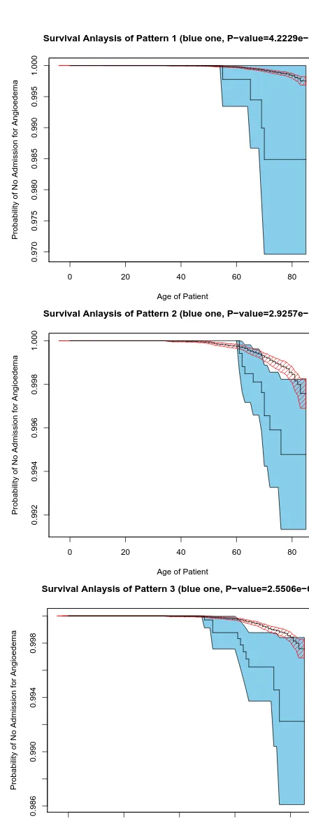
Most found patterns are of great interest to domain experts and verified by them. We have conducted further statistical analysis, e.g. the survival analysis and significance test [16], to evaluate the statistical significance of found patterns.
The survival analysis is concerned with the modelling of ‘life-time’ data. We estimate the survivor functionS(t), by the prob-ability of non-admission to hospitals for Angioedema at aget, to distinguish the subgroup described by the pattern from the others. In addition, we use log-rank test, a formal measure of the strength of evidence that two populations have different lifetimes. It is to detect a difference between groups when the survival curve is con-sistently higher for one group than another.
0 20 40 60 80
0.970
0.975
0.980
0.985
0.990
0.995
1.000
Survival Anlaysis of Pattern 1 (blue one, P−value=4.2229e−09)
Age of Patient
Probability of No Admission for Angioedema
0 20 40 60 80
0.992
0.994
0.996
0.998
1.000
Survival Anlaysis of Pattern 2 (blue one, P−value=2.9257e−05)
Age of Patient
Probability of No Admission for Angioedema
0 20 40 60 80
0.986
0.990
0.994
0.998
Survival Anlaysis of Pattern 3 (blue one, P−value=2.5506e−09)
Age of Patient
[image:5.619.320.541.48.634.2]Probability of No Admission for Angioedema
Figure 1 presents the estimated survivor functions of the groups identified by patterns (within the filled blue regions) and the other patients (within the shaded red regions). Filled blue regions and the shaded red regions indicate their confidence intervals respec-tively. Clearly, for the age 50 and above, the groups identified by patterns have significantly higher probability of hospital admission for Angioedema than the other patients.
A pattern is statistically significant if it has a low value. The P-values of the log-rank test of the patterns are much lower than 0.01. For example, P-values for the above three patterns are4.2×10−9, 2.5×10⁻⁵and2.6×10−9respectively. This also suggests that the sub-groups described by patterns are overwhelmingly different from the other patients.
Both statistical evaluations conclude that the proposed method is able to find statistically significant patterns from a large and skewed data sets.
In the final presentation, we show evolution of relative risk of each pattern, and some patterns that are not in the optimal risk pat-tern set will be rediscovered. An example for showing evolution of Pattern 1 is shown in Figure 2
Pattern 1: RR = 3.99 Gender = Female
Hospital Circulatory Flag = Yes
Usage of Drugs in category “Various” = Yes
Sub pattern: RR = 1.82 Gender = Female
Hospital Circulatory Flag = Yes
Sub pattern: RR = 1.53 Gender = Female
Figure 2: A user interesting evolution path of Risk Pattern 1
6.
CONCLUSIONS
We have discussed a new problem of finding risk patterns in medical data. We have made use of an epidemiological metric, relative risk, in measuring interestingness of patterns and have con-cluded it is an optimal rule mining problem to find high risk pat-terns. We have studied an anti-monotone property for the optimal risk pattern set, and then presented an efficient algorithm to mine optimal risk pattern sets. We applied the method to a real world medical and pharmaceutical linked data set and has revealed some patterns potentially useful in clinical practice.
ACKNOWLEDGEMENTS
This research has been supported by the RGC Earmarked Research Grant of HKSAR CUHK 4179/01E, the Innovation and Technology Fund (ITF) in the HKSAR [ITS/069/03], and ARC DP0559090.
7.
REFERENCES
[1] http://servers.medlib.hscbklyn.edu/ebm/toc.html. [2] R. Bayardo and R. Agrawal. Mining the most interesting
rules. In Proceedings of the Fifth ACM SIGKDD
International Conference on Knowledge Discovery and Data Mining, pages 145–154, N.Y., 1999. ACM Press.
[3] G. V. Belle. Statistical rules of thumb. Wiley-Interscience, New York, 2002.
[4] S. E. Brossette, A. P. Sprague, J. M. Hardin, K. W. T. Jones, and S. A. Moser. Associarion rules and data mining in hospital infection control and public health surveillance.
Journal of American Medical Informatics Association, pages
373 – 381, 1998.
[5] J. Chen, H. He, G. J. Williams, and H. Jin. Temporal sequence associations for rare events. In Advances in
Knowledge Discovery and Data Mining, 8th Pacific-Asia Conference (PAKDD), pages 235–239, 2004.
[6] P. Clark and R. Boswell. Rule induction with CN2: Some recent improvements. In Machine Learning - EWSL-91, pages 151–163, 1991.
[7] P. Clark and T. Niblett. The CN2 induction algorithm.
Machine Learning, 3(4):261–283, 1989.
[8] J. Laurikkala, M. Juhola1, and E. Kentala. Informal identification of outliers in medical data. pages 20 – 24, Berlin, 2000.
[9] J. Li, H. Shen, and R. Topor. Mining the optimal class association rule set. Knowledge-Based System, 15(7):399–405, 2002.
[10] J. Li and L. Wong. Using rules to analyse bio-medical data: A comparison between c4.5 and pcl. In Proc. of Advances in
Web-Age Information Management, pages 254–265, 2003.
[11] M. Ohsaki, S. Kitaguchi, K. Okamoto, H. Yokoi, and T. Yamaguchi. Evaluation of rule interestingness measures with a clinical dataset on hepatitis. In Proceedings of
European Conference on Principles and Practice of Knowledge Discovery in Databases (PKDD), pages
362–373, 2004.
[12] M. Ohsaki, Y. Sato, H. Yokoi, and T. Yamaguchi. A rule discovery support system for sequential medical data in the case study of a chronic hepatitis dataset. In Proc of the
ECML/PKDD-2003 Discovery Challenge Workshop, pages
154 – 165, Cavtat-Dubrovnik, Croatia, 2003.
[13] J. Paetz and R. Brause. A frequent pattern tree approach for rule generation with categorical septic shock patient data. In
Proc of International Symposium of Medical Data Analysis,
pages 207 – 213, 2001.
[14] J. R. Quinlan. Induction of decision trees. Machine Learning, 1(1):81–106, 1986.
[15] J. R. Quinlan. C4.5: Programs for Machine Learning. Morgan Kaufmann, San Mateo, CA, 1993.
[16] S. Selvin. Epidemiologic Analysis — A Case-oriented
Approach. Oxford University Press, New York, 2001.
[17] P. Tan, V. Kumar, and J. Srivastava. Selecting the right objective measure for association analysis. Information
Systems, 29(4):293 – 313, 2004.
[18] M. J. Zaki. Mining non-redundant association rules. Data
Mining and Knowledge Discovery Journal, pages 223–248,
2004.
[19] Z. Zhou and Y. Jiang. Medical diagnosis with c4.5 rule preceded by artificial neural network ensemble. IEEE
Transactions on Information Technology in Biomedicine,