ORPSW: a new classifier for gene expression
data based on optimal risk and preventive patterns
Junpeng Zhang1, Jianfeng He*1, Lei Ma1 and Jiuyong Li2 1
Kunming University of Science and Technology, Kunming, China 2
University of South Australia, South Australia, Australia
Email: {[email protected], [email protected], [email protected], [email protected]}
Abstract—Optimal risk and preventive patterns are itemsets which can identify characteristics of cohorts of individuals who have significantly disproportionate representation in the abnormal and normal groups. In this paper, we propose a new classifier namely ORPSW (Optimal Risk and Preventive Sets with Weights) to classify gene expression data based on optimal risk and preventive patterns. The proposed method has been tested on four bench-mark gene expression data sets to compare with three state-of-the-art classifiers: C4.5, Naive Bayes and SVM. The experiments show that ORPSW classifier is more accurate than C4.5 and Naive Bayes classifiers in general, and is comparable with SVM classifier. Observing that accuracy is sensitive to the prior distribution of the class, we also used false positive rate (FPR) and false negative rate (FNR), to better characterize the performance of classifiers. ORPSW classifier is also very good under this measure. It provides differentially expressed genes in different classes, which help better understand classification process.
Index Terms—Optimal risk and preventive patterns, Weight, Gene expression data, Classifier
I. INTRODUCTION
Microarrays can profile the expression levels of tens of thousands of genes in a sample, which makes it possible to understand the mechanism of disease and be helpful for the diagnosis of disease. However, there are several characteristics in gene expression data which is dramatically different from other data. The number of genes quantified is much larger than the number of samples, which is usually associated with a high risk of over-fitting. Publicly available data set is much small, almost below 100 while the number of genes is normally thousands to tens of thousands. The gene expression data contains noise and redundant information. Therefore, diagnosis methods that are derived from a deep analysis of gene expression profiles are needed. Recently, in the field of machine learning, many methods including C4.5 [1], Naive Bayes [2], SVM(support vector machine) [3], have been used for prediction in gene expression profiles.
C4.5 is one of most popular algorithm in machine learning and often used in gene expression data analysis. It is understandable since a decision tree can be converted to a set of rules. However, C4.5 does not handle imbalanced data
properly when the majority cases belong to one class and tree is not partitioned further. In general, Naive Bayes method uses probabilistic induction to determine class labels of a new or unseen sample, assuming independence among the attributes. It ignores interactions among the attributes. However, interactions between genes are advantageous to improve the accuracy of classification in gene expression data. The ability of SVM for producing a maximal margin hyper-plane and for reducing the amount of training errors has made SVM especially suitable for small sample classification problem, such as gene expression data classification. SVM has good performance, but the biological interpretation of its classification results is poor.
In this paper, we propose a new classifier ORPSW, its classification accuracy is higher than that of C4.5 and Naive Bayes and is comparable with SVM. The strength of our classifier is that it can provide easily understandable weights of each related genes with the class rather than a ‘black box’ embedded in the SVM model.
We have organized this paper in the following order. Section II makes a review of optimal risk and preventive patterns mining. Section III proposes our method including problem definitions, classification by ORPSW, an entropy-based discretization, gene selection entropy-based on CFS (Correlation-based feature selection), and ORPSW classifier. Section IV describes the results of experiment using four gene expression datasets. Section V presents conclusions.
II. AREVIEW OF OPTIMAL RISK AND PREVENTIVE PATTERNS MINING
A. Risk and Preventive Patterns
Gene expression data may be divided into two classes by cancer and normal. Cancer records are also called positive records whereas normal records are negative. In this paper, gene corresponds to attribute and gene expression value to attribute-value. Patterns are defined as a set of one single attribute-value or a set of attribute-values. A risk pattern in this paper refers to the antecedent of a rule with the consequence of cancer and a preventive pattern with the consequence of normal.
In the following we define cancer class as c, normal class as
n and pattern as p.
In public gene expression data, the proportion between cancer and normal is larger than its real proportion. However, the proportion of cancer should be far less than normal. This project supported by Yunnan Fundamental Research Foundation of
Application (No: 2009ZC049M) and Science Research Foundation of Kunming University of Science and Technology (No: 2009-022).
Therefore, the set of support in gene expression data is different from other data. We refer a lsupp (local support) [4] to decide whether a pattern is frequent. The lsupp is described as follows:
) (
) ( )
(
c supp
pc supp c
p
lsupp → = (1)
Where pc is an abbreviation for , others have been called this the recall of the rule . If a pattern’s local support is higher than a given threshold, this pattern is called a frequent pattern.
c p∧
c → p
One of the most often used ratios in epidemiological studies is relative risk or odds ratio [5], which is a concept for the comparison of two groups or populations with respect to a certain undesirable event. For many forms of cancer that are rare, the terms relative risk and odds ratio are interchangeably used because of the approximation. The relative risk measure is conservative: if the relative risk measure is extreme or significant, then the odds ratio is more extreme or more significant [5]. If relative risk is higher than a given threshold, the pattern is more likely to be a risk pattern. Otherwise the pattern is more likely to be a preventive pattern. An example of how to calculate relative risk (RR) and odds ratio (OR) is given as follows.
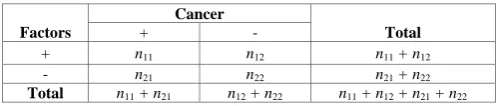
As illustrated in TABLE I, Factors are categorized as positive (+) or negative (-) according to some attribute-value pairs, Cancer is divided as having (+) or not (-) having a certain cancer under investigation. Where n11 and n21 are the number of cancer in positive (+) and negative (-),n12 and n22 are the number of normal in positive (+) and negative (-) respectively.
For instance, if Factor (+) is “Smoking=yes”, Cancer (+) is “lung cancer”, and RR(cancer (+)) =3. We suppose the given threshold is 2. The pattern is a risk pattern because of
RR(cancer (+)) =3>2. It means that a smoking patient is 3 times more risky than non-smoking patient. In contrast, if suppose Factor (+) is “Smoking=no”, Cancer (+) is “lung cancer”, and RR(cancer (+)) =0.3. Because RR(cancer (+)) =0.3<0.5(given threshold of preventive pattern), the pattern composed of the factors is a preventive pattern. It means that “Smoking=no” is more likely irrelevant to “lung cancer”.
) (
) (
)) ( (
12 11 21
22 21 11 22 21
21 12
11 11
n + n n
n + n n = n + n
n ÷ n + n
n = + cancer
RR
12 21
22 11 22 21 12 11 )) ( (
n n
n n
n n ÷ n n cancer
OR + = = (2)
Risk patterns and preventive patterns are formally defined with relative risk as the following.
TABLE I. THE PATTERN IS COMPOSED OF SOME FACTORS FOR JUDGING CANCER OR NOT.
Factors
Cancer
Total
+ -
+ n11 n12 n11 + n12
- n21 n22 n21 + n22
Total n11 + n21 n12 + n22 n11 + n12 + n21 + n22
Definition 1. Risk patterns are frequent patterns, whose
relative risk is greater than a given threshold. Conversely, preventive patterns are frequent patterns, whose relative risk is less than a given threshold.
According to the Definition 1, we should firstly find frequent patterns before finding all risk and preventive patterns. It is noted that the threshold of relative risk in risk patterns is different from that in preventive patterns. The threshold of relative risk in risk patterns is the reciprocal value of that in preventive patterns. Although we can filter out some frequent patterns with relative risk to generate risk and preventive patterns, the number of risk and preventive patterns is still large. Hence it is necessary to further optimize risk and preventive patterns.
B. Optimal Risk and Preventive Patterns
Mining risk and preventive patterns can bring redundant and superfluous patterns. For example, a pattern including two attribute-values “A” and “B” is a risk pattern, its relative risk
is 3.1; another pattern including three attribute-values “A”, “B” and “C” is also a risk pattern, its relative risk is 3.0. In fact, the latter pattern reduces relative risk when incorporated factor “C”. It can be deduced that the former pattern is more optimal compared with the latter pattern. As a result, MORE (Mining Optimal Risk Pattern Sets) algorithm was designed by Li et al [6] for optimal risk and preventive patterns. The reason why optimal risk and preventive patterns can be mined is that optimal risk and preventive patterns set satisfy anti-monotone property. They are proved in [6].
Definition 2. Optimal risk (or preventive) pattern set includes patterns that have higher (or lower in case the relative risk is less than a given threshold) than relative risk of their simple form patterns.
Optimal risk and preventive patterns are extracted from risk and preventive patterns. When the relative risk of risk patterns are less than or equal to that of their sub-patterns and the
relative risk of preventive patterns are more than or equal to that of their sub-patterns, these risk and preventive patterns are ignored.
III. METHODS
A. Problem Definitons
Given a data set with n attributes A1, A2, … , An-1, C. Attributes A1 to An-1 are categorical. Attribute C is a binary class, and one value is covered by our interest, such as disease. The objective of this work is to find out all risk and preventative patterns and then build up a classifier using the summarized patterns to classify future instances. The method of summarized patterns can be divided into two sub-methods: optimal risk and preventive sets, optimal risk and preventive sets with weights.
1) Optimal Risk and Preventive Sets
Let RR1 be relative risk threshold in optimal risk patterns, and RR2 be relative risk threshold in optimal preventive patterns. and are the numbers of attribute-value existed
in RS (Risk Set) and PS (Preventive Set), and are the numbers of attribute-value existed in ORS (Optimal Risk Set) and OPS (Optimal Preventive Set) respectively. Only optimal risk patterns whose relative risk is greater than RR1 and optimal preventive patterns whose relative risk is smaller than
RR2 are selected to generate RS and PS. Common factors between RS and PS are removed. RS (PS) are dealt as the following and remaining factors can produce ORS (OPS).
1
k k2
' k1 k2'
The number of these optimal risk and preventive patterns is and respectively. In addition, we suppose that
, ,
their corresponding RFS (Risk Frequency Set) and PFS
(Preventive Frequency Set) are and
. 1 n RS Pf [ 2 n Ri , 1 Pf , 3 T k Ri ,..., Ri , Ri =[ ] 1 3 2 T k Pf ,..., Pf , ] 2 2 1 T k Pi ,..., Pi , Pi , Pi =
PS [ ]
2 3 2 1 T k Rf ,..., Rf , Rf , Rf ] [ 1 3 2 1
Since that , we should deal with their common attribute-value between RS and PS. We will use the principle of “survival of the fittest” to tackle the common set between RS and PS. The principle of “survival of the fittest” is related with the concept of the grade of membership,which reflects the degree of element in a class, and its value ranges between zero and one [7]. If an attribute-value exists in both sets and the grade of membership of it in RS is more than that in PS, then this attribute-value belongs to RS and should be removed in PS, and vice versa; Particularly, if the grade of membership [7]of it in RS is equal to that in PS, this attribute-value should be removed in both sets. The grade of membership of an attribute-value is the degree belonged to risk factor or preventative factor. If we suppose the frequency of a common attribute-value is CI, the grade of membership is in RS and in PS. Whether the common
attribute-value belongs to RS or not depends on the value of and
.
Φ
PS
RS∩ ≠
2 /n CI 1 /n CI 2 /n CI 1 /n CI
Therefore we can get ORS, ORFS, OPS and OPFS, all of
them meet the condition
that , ,
and . Suppose that
and
, their corresponding
ORFS (Optimal Risk Frequency Set) and OPFS (Optimal Preventive Frequency Set) are [
and . According to Equation (2),
we can generate the relative risk of each attribute-value in
ORS and OPS which are
and
.
Φ
OPS
ORS ∩ =
IPFS PFS⊂ ORi , ORi , ORi
=[ 1 2
OPi , OPi , OPi
=[ 1 2
RS ORS⊂ ' k ORi ,..., 1 3 ' k ,...OPi ] 2 3 RFS ORFS⊂ T ] T ORf , ORf ,
ORf1 2 3
IPS PS⊂ T ' k ORf ,..., ] 1 ORS OPS T ' k OPf ,..., OPf , OPf , OPf ] [ 2 3 2 1 ,..., ORi RR , RR(ORi ,
ORi) ) ( )
( 1 2 3
OPi RR , OPi RR ,
OPi) ( ) ( )
( 1 2 3
T ' k
ORi RR
RR ( )]
[ 1 T ' k OPi ,...RR
RR ( )]
[
2
Definition 3. In optimal risk and preventive sets, only optimal risk patterns whose relative risk is greater than RR1 and optimal preventive patterns whose relative risk is smaller than RR2 are selected to generate optimal risk and preventive set, and there is no common set between optimal risk and preventive set.
For example, suppose we have five risk patterns (RR1=1.5): {R1, R2}( RR=3),
{R1, R2, R3}( RR=3.2), {R2, R5}( RR=5), {R2, R4}( RR=1.4), and {R3, R4, R5}( RR=1.3),
These risk patterns involve five attribute-values: R1, R2, R3, R4, and R5. According to Definition3, only {R1, R2} (RR=3), {R1, R2, R3} (RR=3.2), and {R2, R5} (RR=5) are selected. These selected risk patterns involve four attribute-values: R1, R2, R3, and R5. If these attribute-values still exist in preventive patterns, we can compare grade of membership of them in RS
and PS, and then determine the type of them.
2) Optimal Risk and Preventive Sets with Weights
In this section, we will generate the weight of each attribute-value in ORS and OPS. The weight of each attribute-value in ORS and OPS is represented by RWM (Risk Weight Matrix) and PWM (Preventive Weight Matrix). The weight of each risk factor is the product of its frequency and relative risk
while the weight of each preventative factor is the product of its frequency and the reciprocal of relative risk. RSM and PSM
are described as follows, as in (3) and (4).
Optimal risk and preventive sets with weights are based on optimal risk and preventive sets. We only consider attribute-values in optimal risk and preventive sets. The frequency of each attribute-value can be calculated in optimal risk and preventive patterns and its relative risk can be also obtained according to Equation (2). To make results more intuitive, we normalized the weight of each attribute-value. The total weights of optimal risk and preventative weight are 100 respectively. Each attribute-value in optimal risk and preventive sets has a weight, which generates optimal risk and preventative factor sets with weights respectively.
Definition 4. In optimal risk and preventive sets with weights, the weight of each attribute-value is normalized and related with frequency of it as well as its relative risk.
T ' k j ORi RR ORf ORi RR Rf O ' k j ORi RR ORf ORi RR Rf O ' k j ORi RR ORf ORi RR Rf O RWM j j k j j j j ' k ] 1 = ) ( ) ( 100 ,..., 1 = ) ( ) ( 100 , 1 = ) ( ) ( 100 [ 1 ' 1 2 1
1 2 1 1
1
∑
∑
∑
× × × × × × × × ×T
' k
j RR OPi
OPf
OPi RR OPf
' k
j RROPi
OPf
OPi RR OPf
' k
j RR OPi
OPf
OPi RR OPf PWM
j j
k
j j
j j
' k
]
1
= ( )
1 ) (
1 ×
100
,...,
1
= ( )
1 ) (
1 ×
100 ,
1
= ( )
1 ) (
1 ×
100 [ =
2
' 2
2
2
2
1
2 2
1
∑
∑
∑
××
× ×
× ×
(4)
The Minimal Description Length Principle can be used to stop partitioning. Recursive partitioning within a set of values S stops on the condition:
B. Classification by ORPSW
Our classification first discretizes all individual genes using entropy-based method [8]. Then, we use a gene selection method based on CFS [9] to select most discriminative genes related with class. Finally, we develop ORPSW classifier based on optimal risk and preventive sets with weights. The steps are as follows:
N S T A
N N S
T
A, ; ) log ( 1) ( , ; ) (
ain
G < 2 − +δ (7)
Where N is the number of values in the set S, ,
) ; , E( -) Ent( = ) ; ,
Gain(AT S S AT S δ(A,T;S)=
)] Ent( 2 2• S )
1 k
S −
Ent( )
Ent( [ 2) (3
log2 k − − k• S −k1• ,
and kiis the number of class labels represented in the set Si.
① An entropy-based discretization method: remove those genes that cannot be discretized (Section III-C).
② Gene selection based on CFS: select most discriminative genes (Section III-D).
③ Optimal risk and preventive patterns: these patterns are generated in selected genes using MORE algorithm [6].
Note that this method can be implemented in Weka workbench [10].
D. Gene Selection Based on CFS
Although many noise or irrelevant features are removed in gene expression data after discretization, the number of features is far more than that of samples. Therefore, we incorporate a gene selection method into training data to further explore most discriminatory genes related with the class. This gene selection method is based on CFS and it was proved that it outperformed the wrapper method [11] on small datasets [9].
The key hypothesis of CFS is that good feature sets contain features that are highly correlated with the class, yet uncorrelated with each other. Instead of scoring and ranking individual features, the CFS method uses subset ranking and scoring. Due to best-first-search heuristic, it takes into account the importance of individual features for predicting the class along with the level of inter-correlation among them.
Note that this method can be also implemented in Weka workbench [10].
④ ORPSW classifier: base on optimal risk and preventive sets with weights for classification (Section III-E).
Note that genes with smaller entropy are more discriminating. ORPSW can reduce high-dimensionality of gene expression data and construct classifier based on patterns.
C. An Entropy-Based Discretization Method
One challenge of gene expression data to classification algorithms is the large number of genes involved. It is necessary to remove those irrelevant genes that cannot be discretized based on prior knowledge of class. In this paper, we introduce a discretization method [8] which makes use of the entropy minimization heuristic and derives a criterion based on the Minimum Description Length Principle for deciding split point. This method can remove many noisy or irrelevant genes and explore discriminatory genes related with the class.
We refer the definition described in Fayyad and Irani [8]. Let T partition the set S of examples into the subsets
S1 and S2. Let there be k classes C1,C2,…,Ck and P(Ci,Sj)
be the proportion of examples in Sj that have class Ci. The class entropy of a subset Sj,j=1,2 is defined as:
)) ( )log( 1 (
)
Ent( j i,Sj P Ci,Sj
k
i P C
S ∑
= −
= (5)
E. ORPSW Classifier
ORPSW classifier is implemented based on two main new ideas by two steps. The first is to generate optimal risk and preventive sets with weights; the other is to develop ORPSW classifier.
① We use a new type of knowledge, the so-called optimal risk and preventive patterns, recently proposed in [6], to build up ORPSW classifier. Generally, risk patterns are frequent patterns, whose relative risk [5] is greater than a given threshold. Relative risk is a metric often used in epidemiological studies. It compares the risk of developing a disease of treatment group to control group. Conversely, preventive patterns are frequent patterns, whose relative risk is less than a given threshold. For example, let us consider two patterns. {Gene1 ≥ value1, Gene2 ≥ value2}(lsupp=0.09, RR=3.1), and {Gene1 < value1, Gene2 < value2}(lsupp=0.1, RR=0.1). Where lsupp is local support and RR is relative risk in epidemiology study. The two patterns are risk and Suppose the subsets S1 and S2 are generated by
partitioning a feature A at point T. For example, the test
A>T stands for: “the value of A is greater than T which is a split point”. Then, the class information entropy of the partition, denoted E(A,T;S), is given by:
) ( nt E | |
| | ) ( nt E | |
| | ) ; ,
E( 1 1 2 S2
S S S S S S T
A = + (6)
preventative patterns respectively. Optimal risk (or preventive) pattern set includes patterns that are higher (or lower in case the relative risk is less than a given threshold) than relative risk of their simple form patterns. Therefore, optimal risk and preventive patterns can exclude both redundant and superfluous patterns. In general, the differentiating power of ORPSW classifier roughly depends on the difference of relative risk in target class.
② We use risk weight and preventative weight to classify a new instance. For two classes’ problem, risk weight is risk degree of class C whereas preventative weight is preventative degree of class C. However, it is not reasonable to compare risk weight and preventative weight directly since the number of optimal risk and preventive patterns is different in class. To build up an accurate classifier, we normalize risk weight and preventative weight of each instance with base weight
(e.g. median) of the training instance of class C or non-C
and make comparison, then determine the class of each instance. We let the larger between normalized risk weight and normalized preventative weight win the class.
1) Function of Generating Optimal Risk and Preventive Sets with Weights
Optimal risk and preventive sets with weights are based on optimal risk and preventive patterns. Only optimal risk patterns whose relative risk is greater than
RR1 and optimal preventive patterns whose relative risk is smaller than RR2 are selected, and the grade of
membership is used to remove common set between risk and preventive set. Pseudo-code for generating optimal risk and preventive sets with weight is presented as follows.
Function 1(generating optimal risk and preventive sets with weights).
Input: Optimal risk and preventive patterns (ORPP) generated by MORE algorithm, optimal risk pattern set R, optimal preventive pattern set P, relative risk threshold in optimal risk patterns RR1, and relative risk threshold in optimal preventive patterns RR2.
Output: ORS, RWM (Risk Weight Matrix), OPS and
PWM (Preventive Weight Matrix).
① Set RS,PS,ORS,OPS,RWM,PWM=Φ
② If RR>RR1 (RR<RR2) then add the pattern to R (P) ③ Tabulate optimal risk pattern set (optimal
preventive pattern set) and add the attribute-value in R (P) to RS (PS)
④ If RS∩PS =Φ then ORS= RS, OPS= PS
⑤ Else if RS PS ≠Φ then remove the common attribute-value by the grade of membership
∩
⑥ Return RS and PS then ORS= RS, OPS= PS
⑦ Count the frequency of each attribute-value in
ORS and OPS then sort all attribute-values in order of decreasing frequency
⑧ Calculate the weight of each attribute-value in
ORS and OPS, then add them to RWM and PWM
respectively
⑨ Return RWM and PWM
In step ⑦, we normalize the weight of each attribute-value as described in (3) and (4).
RWM corresponds to ORS, and PWM corresponds to
OPS, which generate optimal risk and preventive sets with weights together.
2) ORPSW Classifier
Given the training samples representing different classes, firstly the classifier is trained and then used to predict new or unseen samples (test samples). ORS, OPS,
RWM and PWM are generated based on training samples. We can use them to predict risk weight and preventative weight of test samples. How do we judge the class of a new sample? A common way is to sum the risk weight and preventative weight, and to compare them. If risk weight is larger than preventative weight, the class of the new sample belongs to cancer, or normal. However, the number of attribute-values in ORS and OPS may not be balanced. If a class has many attribute-values than another class, then the weight of each attribute-value usually gets lower weight.
Our solution to this problem is to “normalize” the weight by base weight. We can judge the class of a new sample though comparing normalized weight. How do we determine the base weight? Suppose two classes C1 and
C2, we can let base_weight (C1) and base_weight (C2) be the median weight of training samples class C1 and C2 respectively. The normalized weight of a new sample s
for C1, norm_weight(s,C1), is defined as the ratio
weight(s,C1)/base_weight (C1). Instead of letting the class with the largest raw weight win, we let the class with the highest normalized weight win. An example is illustrated as follows.
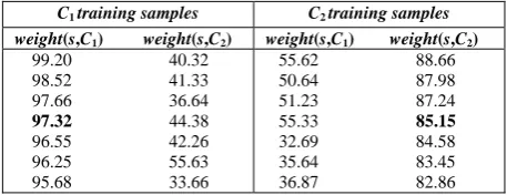
In TABLE II, the (median) base weight for the cancer and normal classes are 97.32 and 85.15 in bold respectively. Given a new sample s with weight 95.20 and 86.65 for the cancer and normal classes respectively, we have norm_weight(s,C1)=95.20/97.32=0.9782 and
norm_weight(s,C2)=86.65/85.15=1.0176. s is labeled as normal.
In summary, ORPSW classifier firstly uses ORS, OPS,
RWM and PWM to generate risk weight and preventative weight of test samples. Then risk weight and preventive weight are normalized based on base weight, a decision made by comparing the value of normalized weight in cancer and normal.
TABLE II. A SIMPLE ILLUSTRATION OF COMPARING PROCESS,
SUPPOSE THERE ARE SEVEN SAMPLES FROM EACH OF THE CANCER (C1) AND NORMAL (C2) CLASSES AND THEIR WEIGHTS ARE:
C1 training samples C2 training samples weight(s,C1) weight(s,C2) weight(s,C1) weight(s,C2)
99.20 40.32 98.52 41.33 97.66 36.64
97.32 44.38 96.55 42.26 96.25 55.63 95.68 33.66
55.62 88.66 50.64 87.98 51.23 87.24 55.33 85.15
IV. EXPERIMENT RESULTS
A. Comparison with Three State-of-the-Art of Classifier
We used four bench-mark gene expression data sets from Kent Ridge Bio-medical Dataset [12] to compare ORPSW with three state-of-the-art of classifiers: C4.5 [1], NB (Naive Bayes) [2] and SVM (Support Vector machine) [3], which are described in TABLE III.
We used two classification performance metrics. The first metric is classification accuracy (ACC) since we wanted to compare our results with three state-of-the art classifiers that also used this performance metric. ACC is easy to reflect the performance of a classifier. On the other hand, ACC is sensitive to the prior distribution of the class and can predict the overall accuracy including true positive rate and true negative rate. In other classification problems, false positives and false negatives makes not much difference, but in cancer diagnosis applications is not the case. False positives are tolerable since further clinical experiments will be done to confirm, but false negatives are unacceptable since a cancer patient might be misclassified as normal. Therefore, the second metric is false positive rate (FPR) and false negative rate (FNR). These two metrics can interpret specificity of a classifier. In cancer classification,
FNR is more useful to evaluate the performance of a classifier.
For ORPSW classifier, we set the minimum local support as lsupp=0.33 in Central Nervous System,
lsupp=0.47 in Breast Cancer, lsupp=0.57 in Prostate Cancer, and lsupp=0.64 in Ovarian Cancer (NCI PBSII Data); the maximum length of the attribute-value item as L=4, the minimum relative risk as 1.5 for optimal risk patterns and as 0.67 for optimal preventive patterns. We firstly discretize four bench-mark gene expression data and then use MORE algorithm [6] to the selected genes to generate optimal risk and preventive patterns. ORPSW classifier can be developed based on optimal risk and preventive patterns. Finally, we make 10-fold stratified cross-validation.
For three state-of-the-arts of classifiers, we also firstly discretize four bench-mark gene expression data, and then make 10-fold stratified cross-validation. Specially, we use two different kinds of SVM which are C-SVC and nu-SVC [13]. The kernel type of them is linear. All our results are obtained by 10-fold stratified cross-validation.
In TABLE IV, the first column is the type of classifier and classification accuracy. Columns from 2 to 5 give the classification accuracy of different classifiers. It can be seen that ORPSW has better predictive accuracy. For Breast Cancer, Ovarian Cancer and Nervous System data sets, ORPSW and SVM (C-SVC+linear) can all achieve 100% testing accuracy. However, Naive Bayes and SVM (nu-SVC+linear) show common performance in four data sets and C4.5 only has 100% testing accuracy in Ovarian Cancer data set. We may conclude that ORPSW classifier can make more accurate classification than C4.5 and Naive Bayes, and is comparable with SVM.
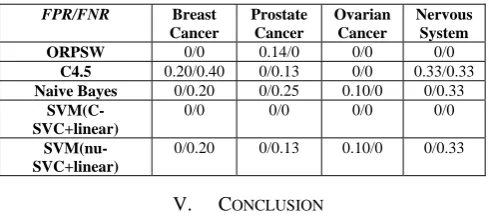
TABLE V gives ORPSW classifier a new metric to compare with other three classifiers on the datasets. The
first column is the type of classifier and FPR/FNR. From the second column to the fifth column, there is FPR/FNR
of different classifiers. It can be shown that ORPSW and SVM (C-SVC+linear) can achieve 0% false negative rate. False negative rate (FNR) is a good metric in cancer classification, which indicates that ORPSW and SVM (C-SVC+linear) are more useful than other types of classifiers in the diagnosis of cancer. On the other hand, C4.5, Naive Bayes and SVM (nu-SVC+linear) have a high false negative rate (FNR) in this case. Thus another conclusion we can infer is that ORPSW classifier is more efficient than C4.5, Naive Bayes and SVM (nu-SVC+linear) in four bench-mark data sets with the lowest average FNR. In Prostate Cancer, ORPSW classifier has the lowest average FNR but the highest average FPR. ORPSW classifier may be over-trained when the fold is 10 in Prostate Cancer.
The primary metric for evaluating classifier performance is classification accuracy (ACC). Since that accuracy (ACC) is sensitive to the prior distribution of the class, we also used false positive rate (FPR) and false negative rate (FNR), to perform a fair and thorough comparison among classifiers. Our experimental results show that ORPSW is an accurate and being better classifier.
A possible reason for ORPSW better than C4.5 decision tree is that it makes use of more attribute information than a decision tree does. C4.5 decision tree only considers optimal rules but ignores sub-optimal rules. A reason for ORPSW better than Naive Bayes may be that Naive Bayes assumes independent among attributes, and ORPSW is not. The assumption ignores interactions between genes which are advantageous to improve the accuracy of classification in gene expression data. Although SVM is mathematically sound, it may be not comprehensive to biologists. The reason is that SVM uses linear or non-linear kernel function to construct a complicated mapping between samples and their class labels and it functions as a black box. However, ORPSW provides relevant genes with the class besides classification performance.
B. Differential Expression Genes Related with the Class
expression value can play different roles in human health. Due to the difference of value in normal and cancer conditions, these genes may have significant impact on classifying patients’ records. Furthermore, these genes may give indications of the biology relevance of disease and provide a treatment plan of the relevant disease.
TABLE III. ASIMPLE DESCRIPTION OF KENT RIDGE BIO-MEDICAL
DATASET.
Name # Samples(training
and testing data)
#Attributes
Central Nervous System 60 7130
Breast Cancer 97 24481
Prostate Cancer 136 12600
Ovarian Cancer(NCI PBSII Data)
253 15154
TABLE IV. CLASSIFICATION COMPARISONS AMONG ORPSW,C4.5,
NAIVE BAYES, AND SVM WITH TWO DIFFERENT TYPES.THE KERNEL TYPE OF SVM IS LINEAR.THE FOLD PARAMETER IS 10.
ACC Breast
Cancer
Prostate Cancer
Ovarian Cancer
Nervous System
ORPSW 1.00 0.93 1.00 1.00
C4.5 0.70 0.93 1.00 0.67
Naive Bayes 0.90 0.86 0.96 0.83
SVM(C-SVC+linear)
1.00 1.00 1.00 1.00
SVM(nu-SVC+linear)
0.90 0.93 0.96 0.83
TABLE V. FPR AND FNR COMPARISONS AMONG ORPSW,C4.5,
NAIVE BAYES, AND SVM WITH TWO DIFFERENT TYPES.THE KERNEL TYPE OF SVM IS LINEAR.THE FOLD PARAMETER IS 10.
FPR/FNR Breast Cancer
Prostate Cancer
Ovarian Cancer
Nervous System
ORPSW 0/0 0.14/0 0/0 0/0
C4.5 0.20/0.40 0/0.13 0/0 0.33/0.33
Naive Bayes 0/0.20 0/0.25 0.10/0 0/0.33
SVM(C-SVC+linear)
0/0 0/0 0/0 0/0
SVM(nu-SVC+linear)
0/0.20 0/0.13 0.10/0 0/0.33
V. CONCLUSION
In this paper, we proposed a new classier based on optimal risk and preventative patterns. Optimal risk (preventive) patterns are characteristics of groups’ people who are risky (preventative) to a disease. ORPSW classifier uses optimal risk and preventive sets with weights to summarize patterns and determine the class label of a new instance by comparing values of normalized weights in cancer and normal groups. Experimental results show that the proposed classifier is useful for cancer classification and helps understand differential expression genes with cancer. The classification results are more accurate than C4.5 and Naive Bayes classifier, and comparable with SVM classifier. Differential expression genes related with the class may provide an indication of the cause of a cancer.
TABLE VI. DIFFERENTIAL EXPRESSION GENES IN TWO BENCH-MARK GENE EXPRESSION DATA SETS:PROSTATE CANCER AND OVARIAN CANCER
(NCIPBSIIDATA).THESE GENES HAVE DIFFERENT EXPRESSION LEVEL IN CANCER AND NORMAL CONDITION.
Prostate Cancer Ovarian Cancer
Genes Cancer Normal Genes Cancer Normal
34730_g_at
37720_at
37068_at
37639_at
32598_at
1121_g_at
36491_at
41468_at
1664_at
39054_at
914_g_at
39608_at
39755_at
(-inf-25.5]
(210.5-inf)
(5.5-inf)
(74.5-inf)
(-inf-29.5]
(-inf-4.5]
(29.5-inf)
(110.5-inf)
(-inf-112]
(-inf-43.5]
(8.5-inf)
(13.5-inf)
(481-inf)
(25.5-inf)
(-inf-210.5]
(-inf-5.5]
(-inf-74.5]
(29.5-inf)
(4.5-inf)
(-inf-29.5]
(-inf-110.5]
(112-inf)
(43.5-inf)
(-inf-8.5]
(-inf-13.5]
(-inf-481]
MZ417.73207
MZ435.07512
MZ435.46452
MZ244.95245
MZ245.53704
MZ246.70832
MZ261.88643
MZ245.24466
MZ246.12233
MZ433.90794
MZ262.18857
MZ17012.128
MZ251.71735
MZ244.66041
(-inf-0.377567]
(0.364727-inf)
(0.339245-inf)
(-inf-0.434996]
(-inf-0.411223]
(-inf-0.23928]
(-inf-0.366697]
(-inf-0.512219]
(-inf-0.341771]
(0.453201-inf)
(-inf-0.408728]
(-inf-0.357613]
(0.269674-inf)
(-inf-0.213234]
(0.480161-inf)
(-inf-0.364727]
(-inf-0.297334]
(0.434996-inf)
(0.411223-inf)
(0.28402-inf)
(0.444799-inf)
(0.512219-inf)
(0.341771-inf)
(-inf-0.453201]
(0.510673-inf)
(0.357613-inf)
(-inf-0.269674]
REFERENCES
[1] Quinlan, J. R, C4.5: Programs for Machine Learning. San Mateo,Calif: Morgan Kaufmann, 1993.
[2] George H. John, P.L, “Estimating Continuous Distributions in Bayesian Classifiers,” Eleventh Conference on Uncertainty in Artificial Intelligence, San Mateo, pp.338-345, 1995.
[3] V.Vapnik, C.C.a, “Support vector machines,” Machine Learning vol.20, pp.273-297, 1995.
[4] Jiuyong Li, A. W.-c. F., Paul Fahey, “Mining Risk Patterns in Medical Data,” Eleventh ACM SIGKDD International Conference on Knowledge Discovery and Data Mining (KDD'05), pp.770-775, 2005.
[5] Selvin.S, Epidemiologic Analysis - A Case-oriented Approach. Oxford University Press, New York, 2001. [6] Jiuyong Li , A. W.-c. F., Paul Fahey, “Efficient discovery
of risk patterns in medical data,” Artificial Intelligence in Medicine vol.45, pp.77-89, 2009.
[7] Zadeh, L, “Fuzzy sets,” Information and control vol.8, pp.338-353, 1965.
[8] Fayyad, U., Irani, K, “Multi-Interval Discretization of Continuous-Valued Attributes for Classification Learning,” Proceedings of the International Joint Conference on Uncertainty in AI, pp.1022-1029, 1993.
[9] Hall, M. A, Correlation-based Feature Selection Machine Learning. PhD thesis Department of Computer Science, University of Waikato, New Zealand, 1998.
[10]Mark Hall, E. F., Geoffrey Holmes, Bernhard Pfahringer, Peter Reutemann, Ian H. Witten, “The WEKA Data Mining Software: An Update,” SIGKDD Explorations vol.11, 2009.
[11]Ron Kohavi, G. H. J, “Wrappers for feature subset selection,” Artificial Intelligence vol.97, pp.273-324, 1997. [12]Jinyan Li, H. L., Limsoon Wong, “Mean-entropy
discretized features are effective for classifying high-dimensional biomedical data,” The 3rd ACM SIGKDD Workshop on Data Mining in Bioinformatics, pp.17-24, 2003.
[13]Chih-Chung Chang, C.-J. L, “LIBSVM - A Library for
Support Vector Machines,” http://www.csie.ntu.edu.tw/~cjlin/libsvm/, 2001.
Junpeng Zhang received his Bachelor’s degree in Bio-medical Engineering in 2009 from Kunming University of Science and Technology, China, and he is currently working for the Master’s degree in Control Theory and Control Engineering from Kunming University of Science and Technology, China. His research interests include Bio-medical data mining and Algorithm design.
Jianfeng He obtained his BSc & MS in electronic engineering from Yunnan University in China 1987 and 1997 respectively, and received his PhD degree in Medical Science from RMIT University in Australia in 2008. He is currently an associate professor at Kunming University of Science and Technology in China. His main research interests are medical imaging process and bioinformatics. His research has been supported by Nature Science Foundation of Yunnan. He has more than twenty journal and conference publications.
search interests are data mining, software engineering.
as more than fifty journal and conference publications.
Lei Ma received his Bachelor in electronics and information engineering from Xiamen University in China in 2001, and received his Master in biomedical engineering (by research) from Monash University in Australia in 2004. He is currently a lecturer of Kunming University of Science and Technology. His major re