Generalized Kruithof approach for traffic matrix estimation

Generalized Kruithof Approach for Traffic Matrix Estimation

Suyong Eum

, Richard. J. Harris

, and Alexander Kist

∗_{School of Electrical and Computer Engineering, Centre for Advanced Technology in Telecommunications (CATT)}

RMIT University, Melbourne, Victoria 3000, Australia, Email:{suyong, kist}@catt.rmit.edu.au

†_{Institute of Information Sciences and Technology, Massey University, Palmerston North,}

Private Bag 11 222, New Zealand,Email: [email protected]

Abstract— In this paper, the traffic matrix estimation problem is formulated as an nonlinear optimization problem based on the generalized Kruithof approach which uses the Kullback distance to measure the probabilistic distance between two traffic matrices. In addition, an algorithm using the affine scaling method is provided to solve the constraint optimization problem. Index Terms— Traffic Matrix, Kruithof Method, Affine Scaling Method, Kullback distance

I. INTRODUCTION

A traffic matrix is defined as a matrix whose elements represent the amount of traffic demand between a given origin to destination node pair in a network. It plays an important role in a variety of network applications such as network dimensioning, planning, optimization, and traffic engineering. However, due to financial and technical difficulties in measur-ing and determinmeasur-ing the traffic matrix directly, an inference approach is the subject of great interest. The methods infer the traffic matrix with the given observed link loads that can be obtained from routers using the SNMP protocol.

Such inference methods rely upon solving systems of equations that are highly under-constrained. The number of unknown variables, which is the number of origin and desti-nation pairs in a network, increases in proportion to the square of the number of nodes while the number of constraints, which is the number of links in a network, increases linearly. Therefore, as the size of the traffic matrix increases, the problem becomes increasingly under-constrained. When a problem is under-constrained, infinite numbers of solutions satisfies the problem. The traffic matrix problem is to find one solution among the infinite numbers of solutions.

Kruithof method [1] has been widely used in telephony network to balance a given fraction matrix with the expected row and column totals. However, the method lacks the ability to accommodate extra information because it was originally introduced to cooperate with the row and column totals only. To address this problem, the Kruithof problem has been generalized as an nonlinear optimization problem [2] using the Kullback distance.

In this paper, the traffic matrix estimation problem is formulated as an nonlinear optimization problem based on the generalized Kruithof approach which uses the Kullback distance to measure the probabilistic distance between two traffic matrices. The idea of the approach is to select one solution among infinite numbers of solutions by minimizing the Kullback distance from the prior solution. The proposed

method is compared with the previously known methods, which are the LP methods [6][7], the least squared [4], and the Information Theory approach [5].

The nonlinear optimization problem is solved using the affine scaling method which is one of the interior point methods which cut across the interior of the feasible area to reach an optimum solution. The affine scaling method is the simplest implementation of all interior point methods, as well as it has the only interior point strategy which approaches a solution by monotonically decreasing the original objective function [3]. We do not provide the detail implementation of the method but a strategy to find a starting point for the affine scaling method by the geometric analysis.

The rest of this paper is organized as follows: In Section II, we explain the under-constrained problem of traffic matrix estimation. Then, in Section III, we explain the theory of our problem formulation. Section IV describes a strategy to accelerate the convergency of the formulated problem by the geometric analysis of the problem. Section V provides the comparison result among deterministic methods. In Section VI, a simulation test-bed is proposed and an experiment is described. Lastly, results and discussions are presented in Section VII.

II. UNDERCONSTRAINTSPROBLEMFORTRAFFIC MATRIXESTIMATION

Estimating a traffic matrix can be described by the vector equation (1).

Y = AX (1)

whereY is the vector of measured link loads,Ais a routing matrix, and X is the vector of traffic demands. In an IP network, the routes can be obtained by noting that most intra-domain routing protocols (eg OSPF and IS-IS) are based on a shortest path algorithm such as the well-known Dijkstra or Bellman-Ford algorithms; also, link volumes in an IP network are typically available from SNMP data. The traffic demands X are unknown, and need to be estimated from the givenY andA. However, it turns out that there may be an infinite set of traffic demands satisfying the given information because linear equation (1) is an under-constrained system. This can be illustrated by the following example.

Fig. 1. 3 node network example.

Fig. 2. Solution space

respectively. The sum of flows 1 and 2 are equal to the measured link load which is 12 and the sum of flow 2 and 3 is the same as the measured link loads 16. The two constraints are illustrated in Fig. 2 based on equations X1+X2 = 12 andX2+X3= 16respectively. This is an under-constrained problem because the number of unknown variables is more than the number of constraints. Therefore, the problem defines a solution plane rather than giving an unique point for the solution. In Fig. 2, the line AB represents the solutions which satisfy both constraints. Whatever technique is used for traffic matrix estimation, a solution from the method should lie on the line AB to satisfy the inter-link measurement constraints.

III. PROBLEMFORMULATION

As mentioned previously, there are infinite numbers of solutions to satisfy the vector equation (1). The traffic matrix estimation problem is to select one of the infinite solutions. The solution is chosen by calculating the closeness from the given prior solution because it is assumed that the prior solution represents some characteristics of the real traffic matrix. The closeness can be represented as the Euclidean distance [4], or the Kullback distance [5]. In other words, when a prior solution is given, a solution is chosen from the feasible area by minimizing the Euclidean or Kullback distance.

We formulated the nonlinear optimization problem using the Kullback distance. It minimizes the Kullback distance between the prior solution and the feasible area, which sat-isfies the constraint (5). The approach is different from the previously suggested method [5] using the Kullback distance. The difference will be discussed in Section V.

Suppose that there are two traffic matricesM andX. The former is a prior traffic matrix, and the latter is the unknown traffic matrix. The both matrices are n×n matrices, and elements of the traffic matrices are represented as lowercase mijandxij. Note thatpij =xij/TXandqij=mij/TM where

TXandTM are total demands denoted by

P_n

i=1

P_n

j=1xijand

Pn i=1

Pn

j=1mij. Therefore, the total sums of pij andqij are

equal to one as follow.

n

X

i=1

n

X

j=1

pij = 1 and n

X

i=1

n

X

j=1

qij = 1 (2)

The probabilistic distance between pij and qij, called

Kullback distanceK(pij, qij), is defined below.

K(pij, qij) = n

X

i=1

n

X

j=1

pijlogpij

qij

(3)

Then, xij/TX and mij/TM are replacing pij and qij

re-spectively. After all, the optimization problem is formulated by minimizing the Kullback distance from the given prior solution to the feasible area, which satisfies the constraint (5).

Minimize

n

X

i=1

n

X

j=1 xij

TX{log

xij

mij −log

TX

TM}

(4)

Subject to

K

X

k=1

A`kX(k)=Y` (`= 1, .., L) ∀X(k)≥0 (5)

where Y is the vector of measured link loads, A is a routing matrix, and X is the vector of traffic demands.

(X = x1

(1,1), x2(1,2), ..., xK(n−−11,n), xK(n,n)) and, K and L are the number of flows and the number of links respectively.

IV. A CHOICE OF THESTARTINGPOINT FORAFFINE SCALINGMETHOD

Any existing interior point method requires a feasible start-ing point, and the choice of the feasible startstart-ing point effects on the convergency speed of the interior point algorithm. In our implementation, the starting point is chosen as follows.

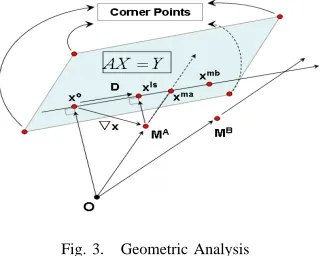
A point x0 _{is selected by minimizing the Euclidean norm} from a zero coordinate O using the pseudo-inverse method x0 _{= A}T_(AAT₎−1_{Y. However, the point is far from the} optimum solution and does not have a physical meaning except it is on the feasible region. The pointx0 needs to be moved to the other feasible point which produces a smaller objective value. From the geometric analysis in Fig.3, the moving direction can be decided.

Fig. 3. Geometric Analysis

Assume that there is a prior solutionMA_{. The optimization}

process is to find a “probabilistically” closest point on the feasible region from the prior solutionMA _{in terms of}

the prior solution MA _{and any point on the line extended}

from lineOMA, is zero.

For instance, if the coordinate of the prior solution MA

is mi (i=1,...,n), any point on the extended line OM A

can be represented as k times mi (k × mi). Therefore,

the Kullback distance between the prior point mi and any

point (k×mi) on the extended line OM A

becomes zero (Pn_i=1Pn_j=1 km_kTij

M{log kmij

mij −log kTM

TM } = 0). If the

ex-tended line OMA goes through the feasible region, the cross point xma _{between the extended line OM}A _{and the}

feasible region becomes the optimum solution. Therefore, the searching direction D to obtain the optimum solution xma

from the pseudo pointx0_{, can be represented as follow.}

D=P∇x= [I−AT_(AAT₎−1_{A]∇x (6)}

whereP =I−AT_(AAT₎−1_{A is the projection matrix into} the null space ofA and∇x= MA_−x0 _(MA _{is the prior}

point andx0 is the pseudo-inverse result). The direction∇x is projected onto the hyperplane which is the feasible region formed byAX=Y so that any movement along the direction D can keep the feasibility. Then, the optimum solution xma is represented as follow.

xma=x0+αD (7)

α is decided by a line search which is one-dimensional minimization technique between0< α < αmax.

αmax=min{−(x

0

i)

Di } (Di∈(Di <0)) (8)

From the basic calculation,αminimizes the objective function f(x0_{+αD) when the directional derivative} d

dαf(x0+αD)

is equal to zero. In this case, the minimum of the objective functionf(x0+αD)is zero so that the point xma becomes the optimum solution (Only one iteration is required to find the optimum solution).

An another case exists to make the problem more complex. Let’s consider another prior solutionMBin Fig.3. In this time, the extended lineOMB does not go through the feasible area. The searching direction D and the line search are applied same as the previous case. Suppose that the point xmb _is

the minimum point from the line search, then the point xmb

can be a starting point for the affine scaling method if all elements of the pointxmb_{are positive. However, the pointx}mb

may contain some negative elements which have no physical meaning. To overcome the problem, Iterative Proportional Fitting (IPF) is applied as suggested in [4].

V. DIFFERENCEFROM THEOTHERDETERMINISTIC APPROACHES

The technique suggested by the authors belongs to the deterministic techniques, which mean that the link load mea-surements are regarded as solid constraints rather than as

statistical data. Table 1 shows the problem formulation of these deterministic approaches with their objective functions and the constraints.

Objective Functions Constaint Linear

Program (M ax)

Pn i=1

Pn

j=1ωijxij Ax≤Y,

Least

Square (M in)

P_n

i=1

P_n

j=1(xij−mij)2

Information Theory (M in)

P_n

i=1

P_n

j=1

xij TX{log

xij

mij} Ax=Y

Generalized Kruithof (M in)

Pn i=1

Pn j=1

xij TX{log

xij mij −log

TX TM}

Table 1.Different deterministic approaches for the traffic matrix estimation

The objective function of the LP approaches [6][7] uses wij as a weight for OD pair xij. When the wij represents

the hop counts of each OD pairxij, the objective function is

parallel to the hyperplane which satisfies the AX =Y. The hop counts of each OD pair is equivalent to the sum of each column ofA. For instance, each column and each row of A represent each flow and each link respectively. Therefore, a column sum of the matrixAmeans how many links the flow, involved the column, goes through.

When the objective function is parallel to the feasible region formed by AX = Y, infinite range of the same optimum solutions are possible. To select one of them as an solution, two main algorithms are available in the LP problem. One is the Simplex Method which chooses an optimum solution from the corner points of the feasible space. The other is the Interior Point Method (IPM) which cuts across the interior of the feasible area to reach an optimum solution.

In Fig. 3, while the Simplex Method selects a solution among the corner points, the iteration of the interior point method starts from any point satisfying with Ax≤ Y, then improves the objective value following a direction which is constant in a linear program (equal to∇xf(x) =wij), since

the objective value decreases most rapidly along this direction. The interior point method chooses a solution which is a cross point between a line extended from the prior solution to the search direction and the feasible region.

For the least square approach [4], after the prior solution MA _{is obtained, a line is drawn perpendicular to the feasible}

region from the prior solution MA_{. The point x}ls_{, which}

is “geographically” closest to the prior solution MA_{, is the}

solution of the least square method.

While the least square approach selects a geographically closest point in the feasible region from the prior solution MA, the information theory [5] and the generalized Kruithof

approach chooses a “probabilistically” closest point defined as the Kullback distance.

extended from lineOMA_.

Therefore, if the extended line OMA _{goes through the}

feasible region, the Kruithof approach selects the pointxma_as

an optimum solution. On the other hands, in the information theory approach case, the point xma _{does not give zero}

objective value, and also is not necessary to be the smallest objective value in the feasible area. In other words, the xma

may not be chosen as the optimum solution. It was also mentioned in [5] that the result of the information theory approach was similar that of the least square method with the square root weight.

Let’s see the below Fig. 4 and Fig. 5, which demonstrate the variation of objective value of the Kruithof approach and the information theory respectively with the given prior solution m1= 1andm2= 1.

Fig. 4. Generalized Kruithof -the objective value by varying two elements x1 and x2 with the given prior solution (m1:1,m2:1)

Fig. 5. Infomation theory - the objective value by varying two ele-ments x1 and x2 with the given prior solution (m1:1,m2:1)

In the Kruithof case in Fig. 4, the objective values are zero along the lineOP because the probabilistic distributions of each point along the line OP ((1,1),(2,2),...,(n,n)) is the same as that of the prior solution (1,1). If the figure is cut vertically following the lineAA0 or BB0 which represents a possible feasible region, the parabola contour defined by the intersection is observed in each case and the parabola contour has the minimum pointE which is one of points on the line OP.

However, in the information theory case in Fig. 5, while the minimum point of the parabola contour by cutting the lineAA0 _{is a pointEon the line OP, the minimum point of}

the parabola contour by cutting the line BB0 _{is not a point}

E but a point somewhere between B and E. It means that the information theory does not choose the point E as an optimum solution even though the pointE has the minimum probabilistic distance to the prior solution. In addition, the objective value of the information theory seems to increase in proportion to the Euclidian distance from the prior point(1,1), then it indicates the objective function of the information theory behaves similar to that of the least square method.

VI. SIMULATIONTOOLS& NETWORKTOPOLOGY

To judge the performance of the proposed method, the linear programming approach, the least squared method, and

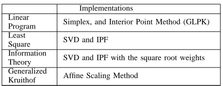
the information theory approach have been implemented. Table 2. outlines the implementations. A simulation program, using theC++ _{language, was built to simulate a network and} to generate traffic distributions for the network.

Implementations Linear

Program Simplex, and Interior Point Method (GLPK) Least

Square SVD and IPF Information

Theory SVD and IPF with the square root weights Generalized

Kruithof Affine Scaling Method

Table 2.Implementation of the deterministic methods

GLPK [8] (GNU Linear Programming Kit), which is an open source libraries, offers C and C++ libraries to solve linear programming and related problems.

The decomposition technique, Single Value Decomposition (SVD), is used to obtain the inverse of the matrix AAT_,

because the normal inversion ofAAT _{can be very numerically}

inaccurate. The inverse of the matrix AAT _{is required to}

obtain the least square resultxls_{and the square root weighted}

least squarexwls_{. In [5], the information theory approach can}

be approximated using the square root weighted least square method.

xls _{= M+A}T_(AAT₎−1_{(Y −AM) (9)} xwls = M+w(Aw)T((Aw)(Bw)T)−1(Y −AM)

where

wij =

p

Mi (i=j)

wij = 0 (i6=j)

M is the given point, and the point is projected on the hyperplane formed by AX = Y. As mentioned previously, the point xls andxwls may contain some negative elements. In that case, IPF is applied to overcome the problem.

To validate those methods, the RMSE (Root Mean Squared Error) and RMSRE (Root Mean Square Relative Error) were used, which provide an overall metric for the errors in the estimates. RMSRE was calculated on the largest 75% of the flows as suggested in [4]. The reason is to protect the RMSRE from being dominated by small flows.

RMSE=

v u u t1

N

N

X

i=1

N

X

j=1

( ˆxij−xij)2 (10)

RMSRE=

v u u t1

N

N

X

i=1

N

X

j=1

{xˆij−xij xij }

2 ₍₁₁₎

topology as that used in [9]. The topology represents the Sprint PoP-level network consisting 70 links.

Fig. 6. Network Topologies

gMatVec [10] was used to manipulate matrices in the implementation of the affine scaling method. gMatVec is a small C++ matrix/vector template library provided by GNU Free Software Foundation.

VII. RESULTSANDDISCUSSION

A. Accuracies of the methods with the variation of the prior solution

The accuracy of each method is dependent on how the prior solution represents the characteristic of the real traffic matrix. For instance, if an old traffic matrix is used as the prior solution, each element of the current traffic matrix is likely to increase proportionally. However, if an estimating technique such as choice model [11] is used to produce a prior solution, the solution becomes close enough to the real solution, so that the solution requires to be refined to satisfy the inter-link measurement constraint.

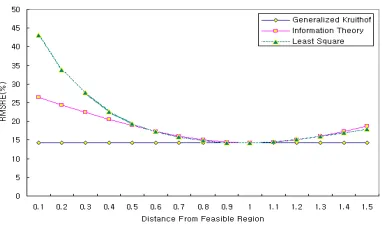
The following figures 7 and 8 show the variations of RMSE and RMSRE of the three different approaches namely the least square, the information theory approach and the generalized Kruithof approach, as the prior solution moves on the extended lineOMA in Fig.3.

Fig. 7. The variation of RMSE as the prior point approaches to the feasible region.

The X-axis of the figures 7 and 8 represent the ratio between the lengthes ofOMA_andOXma_{in Fig.3. Therefore,}

when the prior solution is on the feasible region,OMA _and

OXma _{are matched (The ratio becomes one). The result}

of the generalized Kruithof does not change as the prior

Fig. 8. The variation of RMSE as the prior point approaches to the feasible region.

solution follows the extended line OMA_{, while the RMSE}

and RMSRE of the least square and the information theory decreases, and then increases again after the prior solution passes through the feasible region. The accuracies of the three methods becomes trivial as the prior solution gets closer to the feasible region. It can be seen from the Fig.3, the prior solution MA_{, the least square solutionx}ls_{and the generalized Kruithof}

solutionxkuform a triangle. The triangle becomes smaller as the prior solutionMAis getting closer to the feasible region. That is why the difference of those methods becomes trivial as the prior solution is close to the feasible region.

B. Comparison among the deterministic approaches

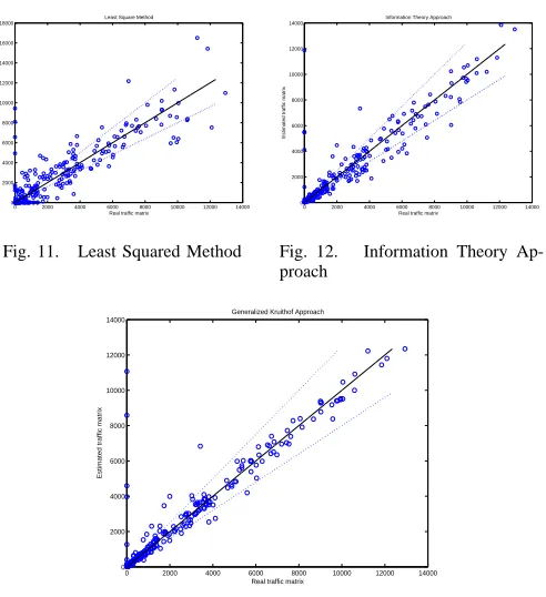
The figures 9,10,11,12, and 13 plot the estimated traffic matrix elements against the synthetic traffic matrix, which is generated artificially according to [7]. The results are obtained when the prior solution has 0.3 distance from the feasible region in Fig 7 and 8. The solid diagonal line shows where the synthetic traffic matrix is estimated exactly and the dotted lines shows±20%of the RMSRE (Root Mean Squared Error) of the estimated flows.

0 2000 4000 6000 8000 10000 12000 14000 0

0.5 1 1.5 2 2.5x 10

4

Real traffic matrix

Estimated traffic matrix

Simplex Method

Fig. 9. Simplex Method

0 2000 4000 6000 8000 10000 12000 14000 0

2000 4000 6000 8000 10000 12000 14000

Real traffic matrix

Estimated traffic matrix

Interior Point Method

Fig. 10. Interior Point Method

0 2000 4000 6000 8000 10000 12000 14000 0

2000 4000 6000 8000 10000 12000 14000 16000 18000

Real traffic matrix

Estimated traffic matrix

Least Square Method

Fig. 11. Least Squared Method

0 2000 4000 6000 8000 10000 12000 14000 0

2000 4000 6000 8000 10000 12000 14000

Real traffic matrix

Estimated traffic matrix

Information Theory Approach

Fig. 12. Information Theory Ap-proach

0 2000 4000 6000 8000 10000 12000 14000 0

2000 4000 6000 8000 10000 12000 14000

Real traffic matrix

Estimated traffic matrix

Generalized Kruithof Approach

Fig. 13. Generalized Kruithof Approach

networks. However, the estimates from the interior point method are scattered along the solid roughly without zero estimation. The interior point method was implemented using the GLPK [8], and it uses a priori solution obtained by [12]. Figures 11, 12, and 13 represent the results of the least square, the information theory approach, and the generalized Kruithof approach respectively. The information theory and the generalized Kruithof approaches estimate the large ele-ments more accurately than the least square method. Specially, in the generalized Kruithof case, large estimated elements are well scattered within the dashed lines.

RMSE RMSRE Simplex Method 4710.6 107.3% Interior Point Method 1333.9 26.4% Least Square Method 1556.2 27.5% Information Theory 1203.7 22.3% Generalized Kruithof 1083.9 14.2%

Table 3.RMSE and RMSRE of deterministic approaches

Table 3 shows the RMSE (Root Mean Square Error) and the RMSRE (Root Mean Square Relative Error) of the de-terministic approaches shown in Fig. 9, 10, 11, 12, and 13. While the simplex method produces over 100 % of RMSRE, the interior point method reduces the RMSRE by more than 70 %. Generalized Kruithof method produced less RMSRE and RMSE around by 8% and by 120 respectively compared to the information theory approach.

VIII. CONCLUSIONS

A new non-linear optimization problem was formulated based on the generalized Kruithof method, which uses the Kullback distance as the measurement of closeness between the given prior solution and a point in the feasible region. The non-linear optimization problem was solved using the affine scaling method which is the simplest implementation of all interior point methods, as well as it has the only interior point strategy which approaches a solution by monotonically decreasing the original objective function.

A strategy to accelerate the convergency of the affine scaling method was developed by the geometric analysis of the problem. The strategy finds a starting point and a searching direction since the choice of these effect the convergency speed of the interior point algorithm.

Four deterministic approaches, which are the simplex method, the interior point method, the least square method, and the information theory approach, have been implemented to compare with the proposed approach. The first two LP ap-proaches show very different results each other (Simplex had an average error of 107.3% while interior point method had 26.4% only) although both use the same problem formulation. The next three methods do not have much different when the given prior solution is close to the feasible region, however the difference becomes noticeable as the prior solution moves far away from the feasible region.

REFERENCES

[1] J. Kruitohf, “Telefoonverkeersrekening. De Ingenieur (’s Gravenhage),”

In ACM SIGMETRICS, no. 8, 19 Feb 1937.

[2] R. Krupp, “Properties of Kruithof’s projection method,” The Bell System

Technical Journal, pp. vol. 58, no. 2, pp. 517–538, Feb 1979.

[3] T. Coleman and L. Yuying, “A trust region and affine scaling interior point method for nonconvex minimization with linear inequality con-straints,” Math Prog, pp. A 88: 1–31, 2000.

[4] Y. Zhang, M. Roughan, N. Duffield, and A. Greenberg, “Fast accurate computation of large-scale IP traffic matrices from link loads,” In ACM

SIGMETRICS, June 2003.

[5] Y. Zhang, M. Roughan, C. Lund, and D. Donoho, “An Information-Theoretic Approach to Traffic Matrix Estimation,” SIGCOMM, August 2003.

[6] O. Goldschmidt, “ISP Backbone Traffic Inference Methods to Support Traffic Engineering,” In Internet Statistics and Metrics Analysis (ISMA)

Workshop, pp. 1063–1075, December 2000.

[7] S. Eum, J. Murphy, and R. Harris, “A Fast Accurate LP Approach for Traffic Matrix Estimation,” International Teletraffic Congress ITC19, 2005.

[8] “GNU Linear Programming Kit.” [Online]. Available: http://directory.fsf.org/libs/glpk.html

[9] A. Nucci, B. Schroeder, S. Bhattacharyya, N. Taft, and C. Diot, “IGP Link Weight Assignment for Transient Link Failures,” International

Teletraffic Congress ITC18, 2003.

[10] “C++ matrix/vector template library.” [Online]. Available: http://gama.fsv.cvut.cz/ cepek/matvec/doc/html/

[11] A. Medina, N. Taft, K. Salamatian, S. Bhattacharyya, and C. Diot, “Traffic Matrix Estimation: Existing Techniques and New Directions,”

ACM SIGCOMM, August 2002.