Droop-Controlled Inverter-Based Microgrids
.
White Rose Research Online URL for this paper:
http://eprints.whiterose.ac.uk/92374/
Version: Accepted Version
Article:
Efimov, D, Schiffer, JF and Ortega, R (2016) Robustness of Delayed Multistable Systems
with Application to Droop-Controlled Inverter-Based Microgrids. International Journal of
Control, 89 (5). pp. 909-918. ISSN 0020-7179
https://doi.org/10.1080/00207179.2015.1104555
[email protected] https://eprints.whiterose.ac.uk/
Reuse
Unless indicated otherwise, fulltext items are protected by copyright with all rights reserved. The copyright exception in section 29 of the Copyright, Designs and Patents Act 1988 allows the making of a single copy solely for the purpose of non-commercial research or private study within the limits of fair dealing. The publisher or other rights-holder may allow further reproduction and re-use of this version - refer to the White Rose Research Online record for this item. Where records identify the publisher as the copyright holder, users can verify any specific terms of use on the publisher’s website.
Takedown
If you consider content in White Rose Research Online to be in breach of UK law, please notify us by
Robustness of delayed multistable systems with
application to droop-controlled inverter-based
microgrids
Denis Efimov, Johannes Schiffer and Romeo Ortega
Abstract
Motivated by the problem of phase-locking in droop-controlled inverter-based microgrids with delays, the recently developed theory of input-to-state stability (ISS) for multistable systems is extended to the case of multistable systems with delayed dynamics. Sufficient conditions for ISS of delayed systems are presented using Lyapunov-Razumikhin functions. It is shown that ISS multistable systems are robust with respect to delays in a feedback. The derived theory is applied to two examples. First, the ISS property is established for the model of a nonlinear pendulum and delay-dependent robustness conditions are derived. Second, it is shown that, under certain assumptions, the problem of phase-locking analysis in droop-controlled inverter-based microgrids with delays can be reduced to the stability investigation of the nonlinear pendulum. For this case, corresponding delay-dependent conditions for asymptotic phase-locking are given.
I. INTRODUCTION
The increasing penetration of renewable distributed generation (DG) units at the low and medium voltage levels has a strong impact on the power system structure [13], [44], [12]. This fact requires new control and operation strategies to ensure a reliable and efficient electrical power supply [13], [16]. An emerging concept to address these challenges is the microgrid [22], [19], [13]. A microgrid is a locally controllable subset of a larger electrical network. It is composed of several DG units, storage devices and loads.
Typically, most DG units in an AC microgrid are connected to the network via AC inverters [16]. Under ideal conditions, an inverter-based DG unit can be modeled as an ideal controllable voltage source [23], [32]. Furthermore, a popular control scheme to operate inverter-based DG units with the purpose to achieve frequency synchronization and power sharing in the network is droop control [6], [18]. Conditions for stability in droop-controlled microgrids with inverters modeled as ideal controllable voltage sources have been derived, e.g., in [36], [34], [26].
In general, inverter-based microgrids operated with droop control have several equilibria [36], [34]. Thus they are multistable systems. Stability analysis [4], [11], [43], [25], [27], [30], [31], [33], [37] and robust stability analysis [1], [3], [5], [7], [41] for this class of systems is rather complicated. Recently, the ISS theory [39] has been extended to multistable systems in [2], [3] (see also [20] for discussion on ISS property with respect to an unbounded set).
Furthermore, in a practical setup, the droop control scheme is applied to an inverter by means of digital discrete time control. Besides clock drifts, see, e.g. [35], digital control usually introduces time delays [21], [24], [28]. According to [28], the main reasons for this are 1) sampling of control variables, 2) calculation time of the digital controller and 3) generation of the pulse-width modulation. We refer the reader to, e.g. [28] for further details. To the best of the authors’ knowledge this fact has yet not been considered in previous analysis of droop-controlled microgrids.
Motivated by the abovementioned phenomenon, the main theoretical contribution of the present paper is to extend the recently derived ISS framework for multistable systems [2], [3] to multistable systems with delay (some preliminary consideration has
Denis Efimov is with with Non-A team @ Inria, Parc Scientifique de la Haute Borne, 40 avenue Halley, 59650 Villeneuve d’Ascq, France, with CRIStAL (UMR-CNRS 9189), Ecole Centrale de Lille, Avenue Paul Langevin, 59651 Villeneuve d’Ascq, France and Department of Control Systems and Informatics, University ITMO, 49 avenue Kronverkskiy, 197101 Saint Petersburg, Russia.
Johannes Schiffer is with Technische Universität Berlin, Einsteinufer 11, 10587 Berlin, Germany.
Romeo Ortega is with Laboratoire des Signaux et Systémes, École Supérieure d’Electricité (SUPELEC), Gif-sur-Yvette 91192, France.
been performed by the authors in [10]). In particular, sufficient conditions for ISS of multistable systems in the presence of delays are given in terms of a Lyapunov-Razumikhin function. It is also shown that ISS multistable systems are robust with respect to feedback delays. This result is illustrated via the example of a nonlinear pendulum. We would like to point out that related works on ISS of time-delay systems by employing Lyapunov functions [8], [15], [29] is limited to systems with a single equilibrium point or a compact attracting set. Next, based on the established results, we provide the main practical contribution: a condition for asymptotic phase-locking in a microgrid composed of two droop-controlled inverters with delay. The analysis is conducted for a simplified inverter model derived under the assumptions of constant voltage amplitudes and ideal clocks, as well as negligible dynamics of the internal inverter filter and controllers. In that scenario, the delay merely affects the phase angle of the inverter output voltage. The stability results are illustrated by simulations.
II. PRELIMINARIES
For an n-dimensional C2 connected and orientable Riemannian manifold M without a boundary, let the map f(x, d) :
M ×Rm→T
xM be of classC1, and consider a nonlinear system of the following form: ˙
x(t) =f(x(t), d(t)), (1)
where the state x∈M andd(t)∈Rm (the input d(·) is a locally essentially bounded and measurable signal) fort≥0. We
denote by X(t, x0;d) the uniquely defined solution of (1) at time t fulfilling X(0, x0;d) = x0. Together with (1) we will
analyze its unperturbed version:
˙
x(t) =f(x(t),0). (2)
A set S⊂M is invariant for the unperturbed system (2) ifX(t, x; 0)∈S for allt∈Rand for allx∈S. Define the distance
from a pointx∈M to the setS⊂M as|x|S = mina∈Sδ(x, a), where the symbolδ(x1, x2)denotes the Riemannian distance
between x1 and x2 inM,|x|=|x|{0} for x∈M or a usual euclidean norm of a vector x∈Rn. For a signald:R→Rm the essential supremum norm is defined as kdk∞=esssupt≥0|d(t)|.
A. Decomposable sets
Let Λ⊂M be a compact invariant set for (2).
Definition 1. [27] A decomposition ofΛis a finite and disjoint family of compact invariant sets Λ1, . . . ,Λk such that
Λ = k
[
i=1
Λi.
For an invariant set Λ, its attracting and repulsing subsets are defined as follows:
A(Λ) ={x∈M :|X(t, x,0)|Λ→0ast→+∞}, R(Λ) ={x∈M :|X(t, x,0)|Λ→0ast→ −∞}.
Define a relation onW ⊂M andD ⊂M byW ≺ D ifA(W)∩R(D)6=⊘.
Definition 2. [27] LetΛ1, . . . ,Λk be a decomposition ofΛ, then
1.An r-cycle (r≥2) is an ordered r-tuple of distinct indicesi1, . . . , ir such that Λi1 ≺. . .≺Λir ≺Λi1.
2.A1-cycle is an indexisuch that [R(Λi)∩A(Λi)]−Λi6=⊘.
3.A filtration ordering is a numbering of theΛi so thatΛi≺Λj ⇒i≤j.
As we can conclude from Definition 2, existence of anr-cycle withr≥2 is equivalent to existence of a heteroclinic cycle for (2) [17]. Furthermore, existence of a1-cycle implies existence of a homoclinic cycle for (2) [17].
Definition 3. The setW is called decomposable if it admits a finite decomposition without cycles, W=Ski=1Wi, for some
B. Robustness notions
The following robustness notions for systems represented by (1) have been introduced in [2], [3] (see also [9] for a survey on ISS framework).
Definition 4. We say that the system (1) has the practical asymptotic gain (pAG) property if there exist η ∈ K∞ and a non-negative real q such that for all x∈M and all measurable essentially bounded inputsd(·)the solutions are defined for all t≥0 and the following holds:
lim sup
t→+∞ |X(t, x;d)|W ≤η(kdk∞) +q. If q= 0, then we say that the asymptotic gain (AG) property holds.
Definition 5. We say that the system (1) has the limit property (LIM) with respect toW if there existsµ∈ K∞ such that for all x∈M and all measurable essentially bounded inputsd(·)the solutions are defined for allt≥0 and the following holds:
inf
t≥0|X(t, x;d)|W≤µ(kdk∞).
Definition 6. We say that the system (1) has the practical global stability (pGS) property with respect to W if there exist
β ∈ K∞ andq≥0such that for all x∈M and measurable essentially bounded inputsd(·)the following holds for allt≥0:
|X(t, x;d)|W≤q+β(max{|x|W,kdk∞}).
It has been shown in [2], [3] that to characterize pAG property in terms of Lyapunov functions the following notion is appropriate.
Definition 7. We say that aC1functionV :M →Ris a practical ISS-Lyapunov function for (1) if there existsK∞functions
α1,[α2], α3 andγ, and scalarq≥0 [andc≥0] such that
α1(|x|W)≤V(x)≤[α2(|x|W+c)], the function V is constant on eachWi and the following dissipation holds:
DV(x)f(x, d)≤ −α3(|x|W) +γ(|d|) +q. If the latter inequality holds forq= 0, thenV is said to be an ISS-Lyapunov function.
Notice that α2 and c are in square brackets as their existence follows (without any additional assumptions) by standard
continuity arguments.
The main result of [2], [3] connecting these robust stability properties is stated below, it extends the results of [38], [40] obtained for connected sets.
Theorem 1. Consider a nonlinear system as in (1) and let a compact invariant set containing all α- andω-limit sets of (2)
W be decomposable (in the sense of Definition 3). Then the following facts are equivalent.
1.The system admits an ISS Lyapunov function;
2.The system enjoys the AG property;
3.The system admits a practical ISS Lyapunov function;
4.The system enjoys the pAG property;
5.The system enjoys the LIM property and the pGS.
Definition 8. [3] Suppose that a nonlinear system as in (1) satisfies the assumptions and the list of equivalent properties of
Theorem 1. Then this system is called ISS with respect to the set W .
III. MULTISTABLE SYSTEMS WITH DELAYS
Letτ >0, for a functiond: [−τ,+∞)→Rmandt≥0denote a functiondt(·) : [−τ,0]→Rmdefined bydt(θ) =d(t+θ)
differential equation on an n-dimensionalC2 connected and orientable Riemannian manifoldM without a boundary:
˙
x(t) =F(xt, dt), x0∈ Cτ, (3)
where the map F :Cτ× D →TxM is of class C1 (we will denote a set of continuous functionsξ : [−τ,0]→ M by Cτ), x(t)∈M is the state,xt∈ Cτ anddt∈ Dfor allt≥0. We denote byX(t, x0;d)the uniquely defined solution of (3) at time
t fulfilling X(θ, x0;d) =x0(θ)for allθ∈[−τ,0];Xtx0,d(θ) =X(t+θ, x0;d)forθ∈[−τ,0]. Define as in [42]
|xt|= max
θ∈[−τ,0]|x(t+θ)|, ||x||t0 = supt≥t0|xt|= supt≥t0−τ|x(t)|.
Again, together with (3), we will analyze its unperturbed version:
˙
x(t) =F(xt,0). (4)
A setS ⊂ Cτ is invariant for the unperturbed system (4) ifXtx0,0∈ S for allt∈R+ and for allx0∈ S. Define the distance
from a function ξ∈ Cτ to a setS ⊂ Cτ as ||ξ||S = minα∈S|ξ−α|.
Let W ⊂M be a set, denote by z}|{W a subset of W ={ξ ∈ Cτ : ξ(t) ∈ W ∀t ∈ [−τ,0]} such that if ζ ∈
z}|{
W then
ζ =Xξ,0
τ for ξ∈ W. For stability analysis in time-delay systems it is required to define a distance to invariant sets in two
spaces: in Rn with respect to the setW and inC
τ with respect to corresponding invariant set
z}|{
W (functions fromCτ taking
values in W and solutions of (3)). The following stability notions for (3) are considered in this work (for a recent survey on stability tools for time-delay systems see [15]).
Definition 9. The system (3) has the pAG property with respect to the setW if there existη∈ K∞ and a non-negative real
q such that for all x0∈ Cτ and all bounded piecewise continuous inputsd(·) the solutions are defined for allt≥0 and the
following holds:
lim sup
t→+∞ |X(t, x0;d)|W ≤η(kdtk0) +q. If q= 0, then we say that the AG property holds.
This property can be equivalently stated as
lim sup t→+∞ ||X
x0,d
t ||z}|{
W ≤
η(kdtk0) +q
and it implies that (a subset of) z}|{W is invariant for (4) ifq= 0.
Definition 10. The system (3) has the pGS property with respect to the setW if there existβ ∈ K∞ andq≥0such that for all x0∈ Cτ and all bounded piecewise continuous inputsd(·) the following holds for allt≥0:
|X(t, x0;d)|W≤q+β(max{||x0||z}|{
W
,kdtk0}).
To characterize pAG and pGS properties for a time-delay system (3) the Lyapunov-Razumikhin approach is used in this work [29], [8]. Given a continuous function x: [−τ,+∞)→M with aC1 functionU :M →RdenoteU(t) =U(x(t)), if
x(t) =X(t, x0;d)is a solution to (3) for some piecewise continuousd: [−τ,+∞)→Rmand initial conditionx0∈ Cτ, then
the upper right-hand side derivative ofU along this solution is
D+U(t) = lim sup h→0+
U(t+h)−U(t)
h .
K∞ functionsα1,[α2], α4, γ andγU,γU(s)< sfor alls >0, and scalarq≥0[andc≥0] such that α1(|x|W)≤U(x)≤[α2(|x|W+c)],
U(t)≥max{γU(|Ut|), γ(|dt|), q} ⇒ D+U(t)≤ −α4[U(t)].
If the latter inequality holds forq= 0, thenU is said to be an ISS-LR function.
Definition 12. The system in (3) is said to be ISS with respect to the setWif it admits pAG and pGS properties with respect
to the set W.
Note that definitions 8 and 12 introduce the same property, but for different classes of systems, (1) and (3), respectively. The following result can be stated connecting pAG, pGS properties and the existence of an ISS-LR function.
Theorem 2. Consider the system (3). Suppose there exists an ISS-LR function U : M → R as in Definition 11. Then the system (3) admits the pAG property from Definition 9 withη(s) =α−11◦γ(s)and the pGS property from Definition 10.
Proof. By using Lemma 1 of [42] and Definition 11, it follows that for allt≥0:
U(t)≤max{χ[U(0), t], γU(||Ut||0), γ(||dt||0), q} (5)
for some χ∈ KL (χ(s,0)≥sfor alls≥0). In addition, forϕ(s) = 0.5[1−sign(s−τ)]:
|Ut| ≤max{|U0|ϕ(t),sup
t≥0
U(t)} (6)
for all t ≥ 0 (this estimate is true by definition of the norm). By substituting (5) in (6) and taking the supremum of the left-hand side of (6) we obtain:
||Ut||0≤max{|U0|ϕ(t), χ[U(0),0], γU(||Ut||0), γ(||dt||0), q}
≤max{χ(|U0|,0), γU(||Ut||0), γ(||dt||0), q}.
Since γU(s)< sfor alls >0 by assumption, the boundedness ofU(t)can be proven [42],i.e.,
||Ut||0≤max{χ(|U0|,0), γ(||dt||0), q}.
From Definition 11, this estimate implies (recall that α(a+b)≤α(2a) +α(2b)for a functionα∈ K for anya≥0,b≥0)
|X(t, x0;d)|W ≤α1−1[max{χ(α2(||x0||z}|{
W
+c),0), γ(||dt||0), q}]
≤max{α−11◦χ(α2(2||x0||z}|{
W
),0), α−11◦γ(||dt||0)}
+α−11◦χ(α2(2c),0) +α−11(q)
≤β(max{||x0||z}|{
W
,||dt||0}) + ˜q,
whereβ(s) =α−11◦max{χ[α2(2s),0], γ(s)}andq˜=α−11◦χ(α2(2c),0) +α−11(q). This implies that the system (3) possesses
the pGS property.
To prove asymptotic convergence considert >2τ, then by substituting (6) in (5) we obtain:
U(t)≤max{χ[U(0), t], γU[sup t≥0
U(t)], γ(||dt||0), q}.
Again γU(s)< sfor alls >0, and for a sufficiently big T >0 [42]:
sup t≥2τ+T
Next, by repeating the arguments given above, asymptotic convergence can be proven, i.e.,
lim sup t→+∞
U(t)≤max{γ(kdtk0), q}, (7)
or, equivalently,
lim sup
t→+∞ |X(t, x0;d)|W ≤α −1
1 ◦γ(kdtk0)] +α−11(q)
completing the proof.
IV. ISSOF MULTISTABLE SYSTEMS WITH DELAYED PERTURBATIONS
In this section we consider the robustness of the system (1) with respect to a disturbanced, which is dependent on a delayed state. The analysis is conducted under the assumption that the system (1) is ISS with respect to a set W. Furthermore, the proposed approach is illustrated via the well-known example of a nonlinear pendulum with delay.
A. Robustness analysis
If (1) is ISS with respect to the set W, then by Theorem 1 there exists an ISS Lyapunov function V as in Definition 7. From the inequalities α3[0.5α−21◦V(x)]≤α3(0.5[|x|W+c])≤α3(|x|W) +α3(c)we obtain
DV(x)f(x, d)≤ −α4[V(x)] +γ(|d|) + ˜q,
whereα4(s) =α3[0.5α−21(s)]andq˜=q+α3(c).
Assume that the input dhas two termsd1 andd2, andd2is a function ofxt∈ Cτ for someτ >0,i.e.:
d=d1+d2, d2=g(xt), (8)
where g is a continuous function,|g(xt)| ≤υ(|Vt|) +υ0 for υ ∈ K∞ and υ0≥0. Denote further for simplicity of notation
d=d1, then the system (1) is transformed to (3) with
F(xt, dt) =f(x(t), d+g(xt)),
and
D+V(t)≤ −α4(V(t)) +γ(2υ(|Vt|) + 2υ0) +γ(2|dt|) + ˜q.
This estimate can be rewritten as follows:
V(t)≥max{ˆγV(|Vt|),γˆ(|dt|),qˆ} ⇒ D+V(t)≤ −0.5α4(V(t)),
ˆ
γV(s) =α−41[6γ(4υ(s))], γˆ(s) =α−41[6γ(2s)],
ˆ
q=α−41[6˜q+ 6γ(4υ0)].
It is straightforward to see that ifγˆV(s)< sfor alls >0, thenV is an ISS-LR function for (1) with (8), and by Theorem 2
this system possesses pAG and pGS properties.
B. Illustration for a nonlinear pendulum
1) Delay-free case: Consider a nonlinear pendulum:
˙
x1 = x2,
˙
x2 = −Ω2sin(x1)−κx2+d,
(9)
where the state x = [x1, x2] takes values on the cylinder M := S×R, d(t) ∈ R is an exogenous disturbance, and Ω, κ
are constant positive parameters. The total energy of (9) is H(x) = 0.5x2
2+ Ω2(1−cos(x1)) and H˙ = x2d−κx22. The
unperturbed system (9) has two equilibria[0,0]and[π,0](the former is attractive and the latter one is a saddle-point). Thus,
W ={[0,0]∪[π,0]} is a compact set containing allα- andω-limit sets of (9) ford= 0. In addition, it is straightforward to check that W is decomposable in the sense of Definition 3.
Lemma 1. The system (9) is ISS with respect to the setW.
Proof. Following the ideas of [5], consider a Lyapunov function candidate
V(x) =H(x) +κǫ(1−cos(x1)) +ǫx2sin(x1), (10)
which is positive definite for any 0.5[κ−√κ2+ 4Ω2]≤ǫ≤0.5[κ+√κ2+ 4Ω2]. Indeed,1−cos(x
1)≥0.5(1−cos2(x1))
for any x1∈S, then
V(x) = 0.5x22+ [Ω2+κǫ](1−cos(x1)) +ǫx2sin(x1)
≥0.5x22+ 0.5[Ω2+κǫ](1−cos2(x1)) +ǫx2sin(x1)
= 0.5x22+ 0.5[Ω2+κǫ] sin2(x1) +ǫx2sin(x1)
= 1 2
h
sin(x1) x2
i
Y
"
sin(x1)
x2
#
,
Y =
"
Ω2+κǫ ǫ
ǫ 1
#
,
and the matrix Y is positive definite for2ǫ∈[κ−√κ2+ 4Ω2, κ+√κ2+ 4Ω2]. Next,
˙
V = x2d−κx22+κǫsin(x1)x2+ǫx22cos(x1)
+ǫsin(x1)[d−Ω2sin(x1)−κx2]
= −[κ−ǫcos(x1)]x22−ǫΩ2sin2(x1) (11)
+ǫsin(x1)d+x2d.
Thus, for further consideration select 0< ǫ≤0.5[κ+√κ2+ 4Ω2], then
˙
V ≤ −0.5[κ−ǫ]x2
2−0.5ǫΩ2sin2(x1) (12)
+0.5[ǫΩ−2+ 1
κ−ǫ]d
2
andV is an ISS Lyapunov function for (9) provided that 0< ǫ <min{κ,0.5[κ+√κ2+ 4Ω2]}=κ. The result follows from
Theorem 1.
Using this result it is possible to prove that for a constant input d(withd <Ω2) the pendulum still has two steady-state
points with similar stability properties.
Lemma 2. Letd <min{Ω2,q̺λmin(Y)
2
π ζ,0.5
√ǫΩπ
ζ, ξ} be a constant input in (9), where ̺= min
κ−ǫ
1 +ǫ,
1
√
2π
ǫΩ2
(Ω2+ (κ+ 1)ǫ)
,
ζ=
r
√
2π[ǫΩ−2+ 1
κ−ǫ], ξ=
2√Ω2+κǫ
ζ
Ω2+ (κ+ 1)ǫ
ǫΩ2 +
1
√
2π̺
and 0< ǫ <min{1, κ}is a parameter. Then the system has two equilibria,[arcsin(dΩ−2),0]and[π−arcsin(dΩ−2),0], the
former one is almost globally attractive.
Proof. It is straightforward to verify that ford <Ω2 the system (9) has two equilibrium points in M. In order to show that
there is no another invariant solution and to investigate stability of these equilibriums we can use ISS property established in Lemma 1. From the proof of Lemma 1 we obtain that for an ISS Lyapunov function V in (10) its derivative satisfies (12) for
0< ǫ < κ. Additionally, from (10) and (12) we have the following series of inequalities:
V(x)≤0.5[(1 +ǫ)x22+ (Ω2+ (κ+ 1)ǫ)x21] ∀x∈M,
˙
V ≤ −0.5[κ−ǫ]x22−0.5
ǫΩ2
√
2πx
2 1
+0.5[ǫΩ−2+ 1
κ−ǫ]d
2 ∀x∈M 1,
V(x)≥0.5[(1−ǫ)x22−(Ω2+ (κ+ 1)ǫ)(x1−π)2]
+2(Ω2+κǫ) ∀x∈M2,
˙
V ≤ −0.5[κ−ǫ]x2 2−0.5
ǫΩ2
√
2π(x1−π)
2
+0.5[ǫΩ−2+ 1
κ−ǫ]d
2
∀x∈M2,
where M1 :={x ∈M : |x1| ≤ 0.5π} and M2 :={x∈M : 0.5π≤x1 ≤1.5π}. Then from the first two inequalities we
obtain for all x∈M1:
˙
V ≤ −̺V + 0.5[ǫΩ−2+ 1
κ−ǫ]d
2
andMd,0={x∈M :V(x)≤0.5̺−1[Ωǫ2 +
1
κ−ǫ]d
2} is an invariant set if it is contained inM
1. From the proof of Lemma 1
we know that
V(x)≥λmin(Y)(x22+ sin2(x1)),
whereλmin(Y) = 0.5(Ω2+κǫ+ 1−
p
(Ω2+κǫ−1)2+ 4ǫ2)is the minimal eigenvalue of the matrixY defined there. Since
V(x)≥λmin(Y) sin2(x1)≥ λmin√2(πY)x21forx∈M1, then we obtain thatMd,0⊂M1if|x1| ≤
q √
2π
2λmin(Y)̺ −1[ ǫ
Ω2 +
1
κ−ǫ]|d| ≤ π
2 or|d| ≤
q
̺λmin(Y)
2
π
ζ. In this caseV(x)≤ π3/2
4√2λmin(Y)forx∈M1.
In the set M2 the function V has a saddle point at [π,0] and the derivative of V is negative-definite outside the set
Md,π ={x∈M2: [κ−ǫ]x22+ ǫΩ
2 √
2π(x1−π)
2 ≤[ǫΩ−2+ 1
κ−ǫ]d
2} andV(x)≥2(Ω2+κǫ)−0.5(Ω2+ (κ+ 1)ǫ)(x 1−π)2
for x∈Md,π if 0< ǫ <min{1, κ}. Note that Md,π⊂M2 for |d| ≤0.5√ǫΩπζ and the levels ofV(x)are separated into the
sets Md,0 andMd,π if|d|< ξ.
Assume that all these restrictions on d are satisfied, i.e. d < min{Ω2,q̺λmin(Y)
2
π ζ,0.5
√ǫΩπ
ζ, ξ}, then by ISS property
asymptotically
lim sup
t→+∞ |x(t)|W≤η(kdk∞)
for some η∈ K∞ withW ={[0,0]∪[π,0]}, and due to compactness of W the variablex(t) is bounded. By consideration above, asymptoticallyx(t)∈Md,0∪Md,πand both equilibriaxa= [arcsin(dΩ−2),0]andxr= [π−arcsin(dΩ−2),0]belong to
this intersection (at these steady-statesx˙ = 0and, hence,V˙ = 0, then all these points are insideMd,0∪Md,πby construction).
Let us show that xa andxrare the only invariant solutions in these sets. For this purpose consider
W(x) = 0.5x22+
p
Ω4−d2+d[arcsin(dΩ−2)
−x1]
−Ω2cos(x1),
thenW :R2→Ris aC1function andW :M →R
+ is a discontinuous one (depending on the definition of the state space).
Note that W(xa) = 0is the global minimum ofW inM ×R, andW(xr) = 2√Ω4−d2+d(2 arcsin(dΩ−2)−π)>0 is a
obtain
˙
W = x2(−Ω2sin(x1)−κx2+d)−dx2+ Ω2sin(x1)x2
= −κx2 2≤0.
Let discontinuity ofW be atx1= 0and consider the setMd,π. Recall thatxris the only steady-state contained inMd,π.Next,
we show by contradiction that xr is the only invariant solution contained in M
d,π. To this end, assume that there is another
positively invariant solution x∗(t)∈M
d,π for all t ≥0. Sincex(t) is bounded, W is continuous on Md,π with a bounded
image and W˙ ≤ 0 for all x∈ Md,π, then by LaSalle’s invariance principle, x∗(t) has to converge to the largest invariant set contained in {x∈Md,π : ˙W ≡0}. Clearly, for x∈ Md,π, W˙ ≡0 implies x(t) =xr for all t ≥0. But xr is a saddle
point and, hence, not attractive. Therefore, xr is the only invariant solution contained in M
d,π. Consequently, any trajectory x(t)withx(0)∈Md,π\ {xr} must exit the set Md,π at some instant in time (since W <˙ 0 there andxr is a saddle of W).
Outside of Md,0∪Md,π we haveV <˙ 0 and it means that the set Md,0 is attractive. To analyze the system behavior inside
the invariant set Md,0, let the discontinuity ofW be at x1=π, again sincex(t)is bounded,W is continuous onMd,0 and
˙
W ≤0, thenx(t)has to converge to the largest invariant set intoW˙ = 0, that isxa.
2) A delayed case study: Now consider a time-delay modification of (9):
˙
x1(t) = x2(t),
˙
x2(t) = −Ω2sin[x1(t−τ)]−κx2(t) +d(t),
(13)
whereτ >0 is a fixed delay. The unperturbed system (13) withd(t) = 0has the same equilibria as (9), i.e.[0,0]and[π,0]. The system (13) can be represented as follows:
˙
x1(t) = x2(t),
˙
x2(t) = −Ω2sin[x1(t)]−κx2(t)
+d(t) + Ω2{sin[x1(t)]−sin[x1(t−τ)]}.
By the mean value theorem
|sin[x1(t)]−sin[x1(t−τ)]|=|cos[x1(φ)]x2(φ)τ|
≤ |x2(φ)|τ
for some φ ∈[t−τ, t]. Thus, the system (13) can be analyzed as a perturbed nonlinear pendulum with part of the input d
dependent on the delay. By taking the estimate derived for V in (11) we obtain forµ=ǫΩ−2+ 1
κ−ǫ:
D+V(t) ≤ −0.5[κ−ǫ]x2
2−0.5ǫΩ2sin2(x1)
+µΩ4x22(φ)τ2+µd2.
It is straightforward to check that
V(x)≤0.5[1 +ǫ]x2
2+ 0.5ǫsin2(x1) + 2[Ω2+κǫ],
x22≤
2
1−ǫV(x) + ǫ
1−ǫ
for 0< ǫ <min{1, κ}, then for ρ= min{κ−ǫ
1+ǫ,Ω
2}
D+V(t) ≤ −ρ{V(t)−2[Ω2+κǫ]}
+µΩ4x22(φ)τ2+µd2
≤ −ρ{V(t)−2[Ω2+κǫ]}
+µΩ
4
1−ǫτ
Therefore,
V(t)≥ 6
ρmax{2 µΩ4
1−ǫτ
2|V
t|,2ρ[Ω2+κǫ] +µΩ
4
1−ǫτ
2ǫ, µd2} ⇒ (14)
D+V(t)≤ −0.5ρV(t)
andV is an ISS-LR function for (13) provided that
12
ρ µΩ4
1−ǫτ
2<1. (15)
The inequality (15) is a delay-dependent stability condition for (13), which is always satisfied for a sufficiently small delay τ. The set of asymptotic attraction for (13) can be evaluated from (14).
Remark 1. If we assume that max{0,κ−Ω2
1+Ω2} < ǫ < min{1, κ}, then min{1+κ−ǫǫ,Ω2} = κ1+−ǫǫ and the condition (15) can be rewritten as follows:
τ2< 1
12Ω2
1−ǫ
1 +ǫ
1
ǫ(κ−ǫ) + Ω2.
Since the functions 1−ǫ
1+ǫ and
1
ǫ(κ−ǫ)+Ω2 are decreasing for ǫ∈(max{0,
κ−Ω2
1+Ω2},min{1, κ}), selectingǫ= max{0,
κ−Ω2
1+Ω2}+ε for a sufficiently small ε >0optimizes the value of the admissible delayτ to
τ∗= 1 2Ω
s
1−ǫ
1 +ǫ
1/3
ǫ(κ−ǫ) + Ω2,
i.e. for anyτ < τ∗ the system (13) admitsV as an ISS-LR function.
V. APPLICATION TO A MICROGRID COMPOSED OF TWO DROOP-CONTROLLED INVERTERS WITH DELAY
In this section the theoretical results of Section III are applied to our main motivating application: a droop-controlled microgrid with delays. In particular, we are interested in conditions for ISS of such systems. In order to tackle this problem, we proceed along the lines detailed in Section IV. The analysis is conducted under a reasonable assumption of constant voltage amplitudes. Then, a lossless droop-controlled microgrid formed by two inverters with delay can be modeled as [34]:
˙
θ(t) = ω1(t)−ω2(t), (16)
τP1ω˙1(t) = −ω1(t)−kP1a12sin[θ(t−τd1)] +c1+d1(t),
τP2ω˙2(t) = −ω2(t) +kP2a12sin[θ(t−τd2)] +c2+d2(t),
whereθ(t)∈[0,2π)is the phase difference in inverters,ω1(t), ω2(t)∈Rare time-varying frequencies of the inverters;τd1>0 and τd2 >0 are delays caused by the digital controls required to implement the droop controls;τP1 >0,τP2 >0,kP1 >0,
kP2 >0,a12>0, c1 andc2=−
kP2
kP1
c1 are constant parameters, the disturbances d1(t)andd2(t)represent additional model
uncertainties. We say that a solution of (16) is phase-locked if θ(t) =θ0 is constant ∀t∈R+ for someθ0 ∈[0,2π)[14]. If
this property holds asymptotically, i.e., for t→+∞, we speak about an asymptotic phase-locking. For brevity of presentation, we impose the following restrictions on the values of parameters.
Assumption 1. τP1 =τP2 =τP >0 andτd1 =τd2 =τ >0.
Under this assumption, define the new coordinates:
x1=θ, x2=ω1−ω2, x3=
kP2
kP1
0 5 10 15 t 2
−
0 2 4
θ
1
ω
2
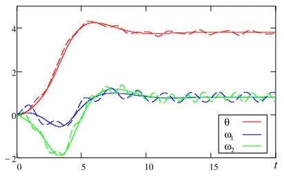
[image:12.612.203.409.53.181.2]ω
Figure 1. Simulation results for the system (16). The solid lines show the state trajectories for the cased1(t) =d2(t) = 0. The dashed lines correspond to the cased1(t) = 0.8 sin(3t),d2(t) = 0.9 sin(5t).
then the system (16) can be rewritten as follows:
˙
x1(t) = x2(t), (17)
τPx˙2(t) = −x2(t)−[kP1+kP2]a12sin[x1(t−τ)]
+[1 +kP2
kP1
]c1+d1−d2, (18)
τPx˙3(t) = −x3(t) +kP2
kP1
d1−d2. (19)
Thus, the system (16) is decomposed into two independent subsystems: (17), (18) and (19). The variable x3 converges
asymptotically to zero with the time constant τP if d1 = d2 = 0. Hence, asymptotically the frequencies ω1 and ω2 are
locked. The dynamics (17), (18) have the form of (13) for d= [1 + kP2
kP1]c1+d1−d2 and, as it has been established above, have pAG and pGS properties from definitions 9 and 10 respectively if condition (15) is satisfied, which for (17), (18) takes the form:
τ2<
minnτ−
1
P −ǫ
1+ǫ ,
[kP1+kP2]a12
τP
o
12[kP1+kP2] 2a2
12
τ2
P(1−ǫ)
h
ǫ
[kP1+kP2]a12 +
1 1−τPǫ
i (20)
for 0< ǫ <min{1, τP−1}. Therefore, for a sufficiently small delay τ the inverters will demonstrate a phase-locking behavior. According to [28], a good estimate of the overall delay introduced by the digital control is τ = 1.75TS1, whereTS = 1/fS
andfS ∈R>0 is the switching frequency of the inverter. Since usually fS ∈[5,20] kHz [16],τ is reasonably small in most
practical applications. Hence, we expect condition (20) to be satisfied for most practical choices of parameters τP, kP1 and
kP2.
The analysis is illustrated in a simulation example with the following set of parameters for the system (16): τP = 1, kP1 = 10, kP2 = 20, a12 = 0.1,c1= 0.2 andτ = 0.05. Condition (20) is satisfied for ǫ= 0.5 min{1, τ
−1
P }. The simulation
results are shown in Fig. 1. The solid lines represent the state (θ, ω1, ω2)T trajectories for the case d1(t) =d2(t) = 0, and
the dashed lines correspond to d1(t) = 0.8 sin(3t),d2(t) = 0.9 sin(5t). The phase-locking phenomenon is observed in these
simulation results.
VI. CONCLUSIONS
Sufficient conditions for ISS of multistable systems with delay have been derived. The conditions have been established using Lyapunov-Razumikhin functions. The potential of the presented approach has been illustrated by exhibiting several new robustness properties for a nonlinear pendulum with delay. Furthermore, it has been shown that asymptotic phase-locking in a lossless droop-controlled microgrid formed by two inverters with delays can be analyzed based on a perturbed pendulum model. By exploiting this fact, a delay-dependent condition for ISS of such a microgrid has been presented.
Future work will consider an extension of the analysis to more complex inverter models with delays (e.g., time-varying voltages or internal filter and controller dynamics).
REFERENCES
[1] D. Angeli. An almost global notion of input-to-state stability. IEEE Trans. Automatic Control, 49:866–874, 2004.
[2] D. Angeli and D. Efimov. On input-to-state stability with respect to decomposable invariant sets. In Proc. 52nd IEEE Conference on Decision and Control, Florence, 2013.
[3] D. Angeli and D. Efimov. Characterizations of input-to-state stability for systems with multiple invariant sets. Automatic Control, IEEE Transactions on, PP(99):1–13, 2015.
[4] D. Angeli, J.E. Ferrell, and E.D. Sontag. Detection of multistability, bifurcations and hysteresis in a large class of biological positive-feedback systems.
Proc. Natl. Acad. Sci. USA, 101:1822–1827, 2004.
[5] D. Angeli and L. Praly. Stability robustness in the presence of exponentially unstable isolated equilibria.IEEE Trans. Automatic Control, 56:1582–1592,
2011.
[6] M.C. Chandorkar, D.M. Divan, and R. Adapa. Control of parallel connected inverters in stand-alone AC supply systems.IEEE Transactions on Industry Applications, 29(1):136 –143, jan/feb 1993.
[7] M. Chaves, T. Eissing, and F. Allgower. Bistable biological systems: A characterization through local compact input-to-state stability. IEEE Trans. Automatic Control, 45:87–100, 2008.
[8] Sergey Dashkovskiy and Lars Naujok. Lyapunov-Razumikhin and Lyapunov-Krasovskii theorems for interconnected ISS time-delay systems. InProc. 19th International Symposium on Mathematical Theory of Networks and Systems(MTNS), pages 1179–1184, Budapest, 2010.
[9] S.N. Dashkovskiy, D.V. Efimov, and E.D. Sontag. Input to state stability and allied system properties.Automation and Remote Control, 72(8):1579–1614,
2011.
[10] Denis Efimov, Romeo Ortega, and Johannes Schiffer. ISS of multistable systems with delays: application to droop-controlled inverter-based microgrids. InProc. ACC 2015, Chicago, 2015.
[11] D.V. Efimov and A.L. Fradkov. Oscillatority of nonlinear systems with static feedback. SIAM Journal on Optimization and Control, 48(2):618–640, 2009.
[12] Xi Fang, Satyajayant Misra, Guoliang Xue, and Dejun Yang. Smart grid - the new and improved power grid: a survey. Communications Surveys & Tutorials, IEEE, 14(4):944–980, 2012.
[13] H. Farhangi. The path of the smart grid. IEEE Power and Energy Magazine, 8(1):18 –28, january-february 2010.
[14] Alessio Franci, Antoine Chaillet, Elena Panteley, and Françoise Lamnabhi-Lagarrigue. Desynchronization and inhibition of Kuramoto oscillators by scalar mean-field feedback.Mathematics of Control, Signals, and Systems, 24(1-2):169–217, 2012.
[15] Emilia Fridman. Tutorial on Lyapunov-based methods for time-delay systems. European Journal of Control, 20:271–283, 2014.
[16] T.C. Green and M. Prodanovic. Control of inverter-based micro-grids. Electric Power Systems Research, Vol. 77(9):1204–1213, july 2007.
[17] J. Guckenheimer and P. Holmes. Structurally stable heteroclinic cycles. Math. Proc. Camb. Phil. Soc., 103:189–192, 1988.
[18] J Guerrero, P Loh, Mukul Chandorkar, and T Lee. Advanced control architectures for intelligent microgrids – part I: Decentralized and hierarchical control.IEEE Transactions on Industrial Electronics, 60(4):1254–1262, 2013.
[19] N. Hatziargyriou, H. Asano, R. Iravani, and C. Marnay. Microgrids. IEEE Power and Energy Magazine, 5(4):78 –94, july-aug. 2007.
[20] Christopher M. Kellett, Fabian R. Wirth, and Peter M. Dower. Input-to-state stability, integral input-to-state stability, and unbounded level sets. InProc. 9th IFAC Symposium on Nonlinear Control Systems, pages 38–43, Toulouse, 2013.
[21] Osman Kukrer. Discrete-time current control of voltage-fed three-phase PWM inverters.IEEE Transactions on Power Electronics, 11(2):260–269, 1996.
[22] R.H. Lasseter. Microgrids. InIEEE Power Engineering Society Winter Meeting, 2002, volume 1, pages 305 – 308 vol.1, 2002.
[23] J.A.P. Lopes, C.L. Moreira, and A.G. Madureira. Defining control strategies for microgrids islanded operation. IEEE Transactions on Power Systems, 21(2):916 – 924, may 2006.
[24] Dragan Maksimovic and Regan Zane. Small-signal discrete-time modeling of digitally controlled PWM converters. IEEE Transactions on Power Electronics, 22(6):2552–2556, 2007.
[25] P. Monzón and R. Potrie. Local and global aspects of almost global stability. InProc. 45th IEEE Conf. on Decision and Control, pages 5120–5125, San Diego, USA, 2006.
[26] Ulrich Münz and Diego Romeres. Region of attraction of power systems. InEstimation and Control of Networked Systems, volume 4, pages 49–54,
2013.
[27] Z. Nitecki and M. Shub. Filtrations, decompositions, and explosions. American Journal of Mathematics, 97(4):1029–1047, 1975.
[28] Thomas Nussbaumer, Marcelo Lobo Heldwein, Guanghai Gong, Simon D Round, and Johann W Kolar. Comparison of prediction techniques to compensate time delays caused by digital control of a three-phase buck-type PWM rectifier system. IEEE Transactions on Industrial Electronics,
55(2):791–799, 2008.
[29] P. Pepe, I. Karafyllis, and Z.-P. Jiang. On the Liapunov-Krasovskii methodology for the ISS of systems described by coupled delay differential and difference equations.Automatica, 44(9):2266–2273, 2008.
[30] R. Rajaram, U. Vaidya, and M. Fardad. Connection between almost everywhere stability of an ODE and advection PDE. InProc. 46th IEEE Conf. Decision and Control, pages 5880–5885, New Orleans, 2007.
[31] A. Rantzer. A dual to Lyapunov’s stability theorem. Syst. Control Lett., 42:161–168, 2001.
[32] Joan Rocabert, Alvaro Luna, Frede Blaabjerg, and Pedro Rodriguez. Control of power converters in AC microgrids. IEEE Transactions on Power Electronics, 27(11):4734–4749, Nov 2012.
[33] V.V. Rumyantsev and A.S. Oziraner. Stability and stabilization of motion with respect to part of variables. Nauka, Moscow, 1987. [in Russian]. [34] Johannes Schiffer, Romeo Ortega, Alessandro Astolfi, Jörg Raisch, and Tevfik Sezi. Conditions for stability of droop-controlled inverter-based microgrids.
Automatica, 2014. Accepted.
[36] J. W. Simpson-Porco, F. Dörfler, and F. Bullo. Synchronization and power sharing for droop-controlled inverters in islanded microgrids. Automatica, 49(9):2603 – 2611, 2013.
[37] S. Smale. Differentiable dynamical systems. Bull. Amer. Math. Soc., 73:747–817, 1967.
[38] E. D. Sontag and Y. Wang. On characterizations of input-to-state stability with respect to compact sets. InProc IFAC Non-Linear Control Systems Design Symposium, (NOLCOS ’95), pages 226–231, Tahoe City, CA, 1995.
[39] E.D. Sontag. On the input-to-state stability property. European J. Control, 1:24–36, 1995.
[40] E.D. Sontag and Y. Wang. New characterizations of input-to-state stability. IEEE Trans. Autom. Control, 41(9):1283–1294, 1996.
[41] G.-B. Stan and R. Sepulchre. Analysis of interconnected oscillators by dissipativity theory. IEEE Trans. Automatic Control, 52:256–270, 2007. [42] Andrew R. Teel. Connections between Razumikhin-type theorems and the ISS nonlinear small gain theorem. IEEE Trans. Automat. Control, 43(7):960–
964, 1998.
[43] R. van Handel. Almost global stochastic stability. SIAM J. Control and Optimization, 45(4):1297–1313, 2006.