Retrieving the time-dependent thermal conductivity of an orthotropic rectangular conductor

This is a repository copy of Retrieving the time-dependent thermal conductivity of an orthotropic rectangular conductor.

White Rose Research Online URL for this paper: http://eprints.whiterose.ac.uk/104370/

Version: Accepted Version

Article:

Hussein, MS, Kinash, N, Lesnic, D et al. (1 more author) (2017) Retrieving the

time-dependent thermal conductivity of an orthotropic rectangular conductor. Applicable Analysis, 96 (15). pp. 2604-2618. ISSN 0003-6811

https://doi.org/10.1080/00036811.2016.1232401

© 2016 Informa UK Limited, trading as Taylor & Francis Group. This is an Accepted Manuscript of an article published by Taylor & Francis in Applicable Analysis on 21st September 2016, available online:

http://www.tandfonline.com/10.1080/00036811.2016.1232401.

[email protected] https://eprints.whiterose.ac.uk/ Reuse

Unless indicated otherwise, fulltext items are protected by copyright with all rights reserved. The copyright exception in section 29 of the Copyright, Designs and Patents Act 1988 allows the making of a single copy solely for the purpose of non-commercial research or private study within the limits of fair dealing. The publisher or other rights-holder may allow further reproduction and re-use of this version - refer to the White Rose Research Online record for this item. Where records identify the publisher as the copyright holder, users can verify any specific terms of use on the publisher’s website.

Takedown

If you consider content in White Rose Research Online to be in breach of UK law, please notify us by

Retrieving the time-dependent thermal conductivity

of an orthotropic rectangular conductor

M.S. Hussein1,2_{, N. Kinash}3_{, D. Lesnic}2 _{and M. Ivanchov}3

1_{Department of Mathematics, College of Science, University of Baghdad, Baghdad, Iraq} 2_{Department of Applied Mathematics, University of Leeds, Leeds LS2 9JT, UK}

3_{Faculty of Mechanics and Mathematics, Department of Differential Equations, Ivan}

Franko National University of Lviv, 1, Universytetska str., Lviv, 79000, Ukraine

E-mails: [email protected] (M.S. Hussein), [email protected] (N. Kinash), [email protected] (D. Lesnic), [email protected] (M.I. Ivanchov).

Abstract

The aim of this paper is to determine the thermal properties of an orthotropic planar structure characterised by the thermal conductivity tensor in the coordinate system of the main directions (Oxy) being diagonal. In particular, we consider retrieving the time-dependent thermal conductivity components of the an orthotropic rectangular conductor from nonlocal overspecified heat flux conditions. Since only boundary measurements are considered, this inverse formulation belongs to the desirable approach of non-destructive testing of materials. The unique solvability of this inverse coefficient problem is proved based on the Schauder fixed point theorem and the theory of Volterra integral equa-tions of the second kind. Furthermore, the numerical reconstruction based on a nonlinear least-squares minimization is performed using the MATLAB optimization toolbox rou-tine lsqnonlin. Numerical results are presented and discussed in order to illustrate the performance of the inversion for orthotropic parameter identification.

Keywords: Orthotropic heat conductor; heat equation; inverse problem; thermal

con-ductivity; regularization.

2010 Mathematics Subject Classification: 65M30, 65M32, 80A23

1

Introduction

Factors such as manufacturing and curing process may affect the material properties of a structure often introducing additional variations such as anisotropy, [4], which are difficult to measure directly. Such a coefficient identification problem is challenging because it is inverse, nonlinear and, in general, ill-posed.

At steady-state, research on the determination of the diffusivity/conductivity of a layered and orthotropic medium has been initiated in [1, 3] and the general case of identi-fication of anisotropic spacewise dependent conductivity in the Laplace-Beltrami elliptic equation has been much investigated in the last two decades, [15].

In the time-dependent case the situation is much less investigated and here we only mention the nonlinear identification of a temperature-dependent orthotropic material, [14], the space-dependent anisotropic case considered in [11], and the recovery of the leading coefficients of a heterogeneous orthotropic medium, [1, 5].

numerically. The inverse problem that we formulate in Section 2 and propose to study combines the features of multi-dimensions, multiple coefficient identification, [6], as well as non-local overdetermination data, [2,7,8,10]. All these papers are unified by the approach utilized to prove the existence of solution: the inverse problem is reformulated as a fixed point problem for a certain nonlinear compact operator, so that the Schauder theorem can be applied to it. Afterwards, uniqueness of solution follows from the theory of Volterra integral equations of the second kind. In this paper, we also follow this approach and prove the existence and uniqueness of the solution in Section 2. The numerical solutions of the direct and inverse problems are described in Section 3 and 4, respectively, and numerical results are presented and discussed in Section 5. Finally, conclusions are given in Section 6.

2

Statement of the problem

We consider an inverse problem of identifying the thermal conductivity coefficients a1(t)

and a2(t) in the two-dimensional orthotropic heat equation

ut=a1(t)uxx+a2(t)uyy +f(x, y, t),

(x, y, t)_∈QT :=_{(x, y, t) : 0 < x < h,0< y < l,0< t < T_}, (1)

with initial condition

u(x, y,0) =φ(x, y), (x, y)_∈[0, h]_×[0, l], (2)

Dirichlet boundary data

u(0, y, t) =µ11(y, t), u(h, y, t) =µ12(y, t), (y, t)∈[0, l]×[0, T], (3)

u(x,0, t) = µ21(x, t), u(x, l, t) =µ22(x, t), (x, t)∈[0, h]×[0, T] (4)

and nonlocal overspecification conditions

a1(t)(ν11(t)ux(0, y0, t) +ν12(t)ux(h, y0, t)) =κ1(t), t ∈[0, T], (5)

a2(t)(ν21(t)uy(x0,0, t) +ν22(t)uy(x0, l, t)) = κ2(t), t∈[0, T], (6)

wherex0, y0 are fixed values from the intervals (0, h) and (0, l) respectively.

Let Gk(x, t, ξ, τ) be the Green function for the equation ut =a1(t)uxx with Dirichlet

boundary conditions fork= 1, and with Neumann boundary conditions fork = 2. These functions are defined by, [9],

Gk(x, t, ξ, τ) =

1

2√π(θ1(t)−θ1(τ)) +∞

∑

n=−∞

(

exp

(

−(x−ξ+ 2nh)

2

4(θ1(t)−θ1(τ))

)

+(₋1)kexp

(

−(x+ξ+ 2nh)

2

4(θ1(t)−θ1(τ))

))

, k = 1,2, θ1(t) =

t

∫

0

a1(τ)dτ, t∈[0, T]. (7)

At the same time we define the function Gm(y, t, η, τ) for the equation ut = a2(t)uyy

analogously toGk(x, t, ξ, τ).

Then the Green function of the problem (1)-(4) is defined by

Theorem 1. Let the following assumptions be satisfied:

(A1) φ _∈C2_{([0, h]×[0, l]), µ}

11, µ12∈C2,1([0, l]×[0, T]), µ21, µ22 ∈C2,1([0, h]×[0, T]),f ∈

C1,0_{(QT), κ}

1,κ2, ν11, ν12 ∈C([0, T]);

(A2) κ_{1(t) > 0, ν11(t) + ν12(t) > 0, t ∈ [0, T], φx(x, y) > 0, (x, y) ∈ [0, h] × [0, l],} µ21x(x, t) > 0, µ22x(x, t) > 0, (x, t) ∈ [0, h] × [0, T], µ11t(y, t) − f(0, y, t) 6 0, µ11yy(y, t) > 0, µ12t(y, t) −f(h, y, t) > 0, µ12yy(y, t) 6 0, (y, t) ∈ [0, l]×[0, T], fx(x, y, t)>0, (x, y, t)∈QT;

(A3) κ_{2(t) > 0, ν21(t) + ν22(t) > 0, t ∈ [0, T], φy(x, y) > 0, (x, y) ∈ [0, h] × [0, l],} µ11y(y, t) > 0, µ12y(y, t) > 0, (y, t) ∈ [0, l] × [0, T], µ21t(x, t) − f(x,0, t) 6 0, µ21xx(x, t) > 0, µ22t(x, t) −f(x, l, t) > 0, µ22xx(x, t) 6 0, (x, t) ∈ [0, h]×[0, T], fy(x, y, t)>0, (x, y, t)_∈QT;

(A4) φ(0, y) = µ11(y,0), φ(h, y) = µ12(y,0), y ∈ [0, l], φ(x,0) = µ21(x,0), φ(x, l) =

µ22(x,0), x ∈ [0, h], µ11(0, t) = µ21(0, t), µ11(l, t) = µ22(0, t), µ12(0, t) = µ21(h, t),

µ12(l, t) = µ22(h, t), t ∈[0, T].

Then the problem (1)-(6) has at least one solution (a1, a2, u)∈(C([0, T]))2×C2,1(QT).

Proof. To prove the existence of a solution to (1)-(6) we are first going to reduce it to an equivalent in a certain sense operator equation with respect to (a1, a2) and afterwards

apply the Schauder fixed point theorem.

If a1(t)>0, a2(t)>0 are known functions, the solution to the direct problem (1)-(4)

can be represented as

u(x, y, t) = h ∫ 0 l ∫ 0

G11(x, y, t, ξ, η,0)φ(ξ, η)dξdη+

l ∫ 0 t ∫ 0

G11ξ(x, y, t,0, η, τ)a1(τ)µ11(η, τ)dηdτ

− l ∫ 0 t ∫ 0

G11ξ(x, y, t, h, η, τ)a1(τ)µ12(η, τ)dηdτ +

h ∫ 0 t ∫ 0

G11η(x, y, t, ξ,0, τ)a2(τ)µ21(ξ, τ)dξdτ

− h ∫ 0 t ∫ 0

G11η(x, y, t, ξ, l, τ)a2(τ)µ22(ξ, τ)dξdτ +

h ∫ 0 l ∫ 0 t ∫ 0

G11(x, y, t, ξ, η, τ)f(ξ, η, τ)dξdηdτ.

(9)

Denote w1 :=ux(x, y, t) and differentiate (9) with respect to x to obtain

w1(x, y, t) =

h ∫ 0 l ∫ 0

G21(x, y, t, ξ, η,0)φξ(ξ, η)dξdη−

l ∫ 0 t ∫ 0

G21(x, y, t,0, η, τ)(µ11τ(η, τ)

−f(0, η, τ)₋a2(τ)µ11ηη(η, τ))dηdτ + l ∫ 0 t ∫ 0

G21(x, y, t, h, η, τ)(µ12τ(η, τ)−f(h, η, τ)

−a2(τ)µ12ηη(η, τ))dηdτ + h ∫ 0 t ∫ 0

− h

∫

0

t

∫

0

G21η(x, y, t, ξ, l, τ)a2(τ)µ22ξ(ξ, τ)dξdτ + h

∫

0

l

∫

0

t

∫

0

G21(x, y, t, ξ, η, τ)fξ(ξ, η, τ)dξdηdτ.

(10)

An operator equation with respect toa1 is obtained from (5) as

a1 =P1(a1, a2), (11)

where

P1(a1, a2)(t) =

κ_1(t)

ν11(t)w1(0, y0, t) +ν12(t)w1(h, y0, t)

, t∈[0, T]

and w1is defined by (10).

Analogously, in order to get an operator equation with respect toa2(t), we differentiate

(9) with respect toy and use the notation w2 :=uy(x, y, t) to obtain

w2(x, y, t) =

h

∫

0

l

∫

0

G12(x, y, t, ξ, η,0)φη(ξ, η)dξdη

+ l

∫

0

t

∫

0

G12ξ(x, y, t,0, η, τ)a1(τ)µ11η(η, τ)dηdτ

− l

∫

0

t

∫

0

G12ξ(x, y, t, h, η, τ)a1(τ)µ12η(η, τ)dηdτ

− h

∫

0

t

∫

0

G12(x, y, t, ξ,0, τ)(µ21τ(ξ, τ)−f(ξ,0, τ)−a1(τ)µ21ξξ(ξ, τ))dξdτ

+ h

∫

0

t

∫

0

G12(x, y, t, ξ, l, τ)(µ22τ(ξ, τ)−f(ξ, l, τ)−a1(τ)µ22ξξ(ξ, τ))dξdτ

+ h

∫

0

l

∫

0

t

∫

0

G12(x, y, t, ξ, η, τ)fη(ξ, η, τ)dξdηdτ. (12)

Therefore, an operator equation with respect toa2 is obtained from (6)

a2 =P2(a1, a2), (13)

where

P2(a1, a2)(t) =

κ_2(t)

ν21(t)w2(x0,0, t) +ν22(t)w2(x0, l, t)

, t ∈[0, T]

and w2 is defined by (12).

Denote:

N := {a1, a2 ∈ C([0, T]) : α1 6 a1(t) 6 A1, α2 6 a2(t) 6 A2}, where the constants

P :_{N → N} such that P(a1, a2) =

(

P1(a1, a2)

P2(a1, a2)

)

.

Thus, the problem (1)-(6) is reduced to the operator equation

(a1, a2) = P(a1, a2), (a1, a2)∈ N. (14)

The problem (1)-(6) is equivalent to the equation (14) in the following sense: if (a1, a2, u) is a solution to (1)-(6), then (a1, a2) is a solution to (14), and, conversely,

if (a1, a2) ∈ N is a solution to (14), then (a1, a2, u) is a solution to (1)-(6), where u is

defined by formula (9). This follows from the way the equation (14) has been obtained. To make sure that the operator P maps _N into itself let us estimate the constants α1, α2, A1, A2 ∈R+. From the uniqueness of the solution to the problem

    

ut=a1(t)uxx, (x, t)∈(0, h)×(0, T),

u(x,0) = 1, x_∈[0, h],

ux(0, t) = 0, ux(h, t) = 0, t _∈[0, T],

the following identity is obtained

h

∫

0

G2(x, t, ξ,0)dξ = 1. (15)

According to the properties of the Green function (namely, that G1η(y, t,0, η)>0, G1η(y, t, l, η)60 and (15) holds) it follows from (A2) applied to (10) that

w1(x, y, t)> min

[0,h]×[0,l]φx(x, y)

l

∫

0

G1(y, t, η,0)dη+ min

[0,h]×[0,T]µ21x(x, t)

t

∫

0

G1η(y, t,0, τ)a2(τ)dτ

− min

[0,h]×[0,T]µ22x(x, t)

t

∫

0

G1η(y, t, l, τ)a2(τ)dτ.

Similarly to (15), from the uniqueness of the solution to the problem

    

ut=a2(t)uyy, (y, t)∈(0, l)×(0, T),

u(y,0) = 1, y_∈[0, l],

u(0, t) = 1, u(l, t) = 1, t _∈[0, T].

we obtain the formula

l

∫

0

G1(y, t, η,0)dξ+

t

∫

0

G1η(y, t,0, τ)a2(τ)dτ −

t

∫

0

G1η(y, t, l, τ)a2(τ)dτ = 1. (16)

The formula (16) implies the estimate

w1(x, y, t)>min{ min

Thus, the following estimate for the operatorP1 holds:

P1(a1, a2)(t)6

max

[0,T]

κ_1(t)

min

[0,T](ν11(t) +ν12(t))W1

=:A1, t∈[0, T].

Similarly,

P2(a1, a2)(t)6A2, t∈[0, T],

where

A2 :=

max

[0,T]

κ_2(t)

min

[0,T](ν21(t) +ν22(t))W2

,

W2 := min{ min

[0,h]×[0,l]φy(x, y),[0,lmin]×[0,T]µ11y(y, t),[0,lmin]×[0,T]µ12y(y, t)}.

The next step is to obtain the upper bound estimate of w1(0, y0, t). It implies from

(15) and (16) that

h ∫ 0 l ∫ 0

G21(x, y, t, ξ, η,0)φξ(ξ, η)dξdη+

h ∫ 0 t ∫ 0

G21η(x, y, t, ξ,0, τ)a2(τ)µ21ξ(ξ, τ)dξdτ

− h ∫ 0 t ∫ 0

G21η(x, y, t, ξ, l, τ)a2(τ)µ22ξ(ξ, τ)dξdτ

6max_{ max

[0,h]×[0,l]φx(x, y),[0,hmax]×[0,T]µ21x(x, t),[0,hmax]×[0,T]µ22x(x, t)}.

It is shown in [9] thatG2(0, t,0, τ)6

(

1 h+

1

√

πα1(t−τ)

)

and G2(0, t, h, τ)6

1

h. Thus,

− l ∫ 0 t ∫ 0

G21(0, y0, t,0, η, τ)(µ11τ(η, τ)−f(0, η, τ)−a2(τ)µ11ηη(η, τ))dηdτ

6

(

T h +

2√T √_πα

1

) (

max

[0,l]×[0,T](−µ11t(y, t) +f(0, y, t)) +A2[0,lmax]×[0,T]µ11yy(y, t)

) ; l ∫ 0 t ∫ 0

G21(0, y0, t, h, η, τ)(µ12τ(η, τ)−f(h, η, τ)−a2(τ)µ12ηη(η, τ))dηdτ

6 1 h

(

max

[0,l]×[0,T](µ12t(y, t)−f(h, y, t)) +A2[0,lmax]×[0,T](−µ12yy(y, t))

)

.

Finally, the last term of (10) is evaluated by

h ∫ 0 l ∫ 0 t ∫ 0

G12(x, y, t, ξ, η, τ)fξ(ξ, η, τ)dξdηdτ 6T max

QT

After the same procedure is applied to w1(h, y0, t), the following inequality is obtained:

ν11(t)w1(0, y0, t) +ν12(t)w1(h, y0, t)6C1+

C2

√_α

1

.

Therefore, for P1 we obtain the lower bound estimate

C3

C1+

C2

√_α

1

6P1(a1, a2)(t), t∈[0, T], where C3 := min [0,T]

κ_1(t).

To ensure thatP maps _N into itself α1 must satisfy the equation

α1 =

C3

C1+

C2

√_α

1

.

This equation has a unique positive solution

α1 :=

(

−C2+

√

C2

2 + 4C1C3

2C1

)2

.

Similarly,

ν21(t)w2(x0,0, t) +ν22(t)w2(x0, l, t)6C4+

C5

√_α

2

,

which yields the lower bound estimate for P2

C6

C4+ √C_α25

6P2(a1, a2)(t), t∈[0, T], whereC6 := min [0,T]

κ_2(t).

Then,α2 satisfies the equation

α2 =

C6

C4+√C5_α2 ,

which has only one positive solution

α2 :=

(

−C5+

√

C2

5 + 4C4C6

2C4

)2

.

Taken such values for α1, α2, A1, A2 ∈ R+, the operator P maps the set N into itself.

Compactness of the operator P follows from [9]. According to the Schauder theorem there exists a solution to (14), and therefore to the problem (1)-(6).

Theorem 2. Provided that κ_{1(t)̸= 0,}κ_{2(t)= 0̸ for t ∈ [0, T], the solution (a1, a2, u) to}

the problem (1)-(6) is unique in C([0, T])2_×C2,1_(Q

Proof. Suppose that there are two solutions (a1(t), a2(t), u(x, y, t)) and

(a∗

1(t), a∗2(t), u∗(x, y, t)) to the problem (1)-(6). Denote ba1(t) = a1(t) − a∗1(t),ba2(t) =

a2(t)−a∗2(t) ub(x, y, t) =u(x, y, t)−u∗(x, y, t). Then (ba1(t),ab2(t),ub(x, y, t)) is solution to

the problem

b

ut=a1(t)ubxx+a2(t)ubyy+ba1(t)u∗xx(x, y, t) +ba2(t)uyy∗ (x, y, t), (x, y, t)∈QT, (17)

b

u(x, y,0) = 0, (x, y)_∈[0, h]_×[0, l], (18)

b

u(0, y, t) = 0, _bu(h, y, t) = 0, (y, t)_∈[0, l]_×[0, T], (19)

b

u(x,0, t) = 0, u_b(x, l, t) = 0, (x, t)∈[0, h]×[0, T], (20)

b

a1(t)(ν11(t)ux∗(0, y0, t) +ν12(t)u∗x(h, y0, t)) +a1(t)(ν11(t)uxb (0, y0, t)

+ν12(t)bux(h, y0, t)) = 0, t∈[0, T], (21)

b

a2(t)(ν21(t)u∗y(x0,0, t) +ν22(t)u∗y(x0, l, t)) +a2(t)(ν21(t)buy(x0,0, t)

+ν22(t)buy(x0, l, t)) = 0, t ∈[0, T]. (22)

The solution to the problem (17)-(20) can be calculated by formula (9) to read

b

u(x, y, t) = t

∫

0

l

∫

0

h

∫

0

G11(x, y, t, ξ, η, τ)(ba1(τ)u∗xx(ξ, η, τ) +ba2(τ)u∗yy(ξ, η, τ))dξdηdτ,

(x, y, t)_∈Q_T. (23)

Substituting (23) into (21), (22) we obtain the system

b

a1(t)(ν11(t)u∗x(0, y0, t) +ν12(t)u∗x(h, y0, t)) =−a1(t)

t

∫

0

l

∫

0

h

∫

0

(ν11(t)G11x(0, y0, t, ξ, η, τ)

+ν12(t)G11x(h, y0, t, ξ, η, τ))(ba1(τ)uxx∗ (ξ, η, τ) +ba2(τ)u∗yy(ξ, η, τ))dξdηdτ, t∈[0, T], (24)

b

a2(t)(ν21(t)u∗y(x0,0, t) +ν22(t)u∗y(x0, l, t)) =−a2(t)

t

∫

0

l

∫

0

h

∫

0

(ν21(t)G11y(x0,0, t, ξ, η, τ)

+ν22(t)G11y(x0, l, t, ξ, η, τ))(ba1(τ)uxx∗ (ξ, η, τ) +ba2(τ)u∗yy(ξ, η, τ))dξdηdτ, t∈[0, T]. (25)

Thus, (24) and (25) form a system of homogeneous Volterra integral equations of the second kind. Since (a∗

1, a∗2, u∗) is solution to the problem (1)–(6), it implies from the

conditions (5), (6) and assumptions of the theorem that

ν11(t)u∗x(0, y0, t) +ν12(t)u∗x(h, y0, t)̸= 0, ν21(t)u∗y(x0,0, t) +ν22(t)u∗y(x0, l, t)̸= 0, t ∈[0, T].

Therefore, the system of equations (24) and (25) has a unique trivial solution. The uniqueness is proved.

3

Solution of direct problem

is to be determined. To achieve this, we use the Forward-Time-Central-Space (FTCS) finite-difference scheme which is conditionally stable.

We subdivide the solution domain QT into Mx, My and N subintervals of equal step lengths ∆xand ∆y, and uniform time step ∆t, where ∆x=h/Mx, ∆y=ℓ/My and ∆t= T /N, for space and time, respectively. At the node (i, j, k) we denoteuk

i,j :=u(Xi, Yj, tk), where Xi =i∆x, Yj = j∆y, tk = k∆t, ak

1 :=a(tk), ak2 :=a2(tk) and fi,jk := f(Xi, Yj, tk) fori= 0, Mx,j = 0, My and k = 0, N.

The simplest explicit difference scheme for equation (1) is given by

uk_i,j+1−uki,j ∆t =a

k

1

uk

i+1,j−2uki,j +uki−1,j (∆x)2 +a

k

2

uk

i,j+1−2uki,j +uki,j−1

(∆y)2 +f

k

i,j (26)

for i = 1, Mx−1, j = 1, My−1 and k = 0, N. The initial and boundary conditions (2)–(4) give

u0_i,j =ϕi,j, i= 0, Mx, j = 0, My, (27) uk_0,j =µ11(Yj, tk), ukMx,j =µ12(Yj, tk), j = 0, My, k= 1, N , (28)

uk_i,0 =µ21(Xi, tk), uki,My =µ22(Xi, tk), i= 0, Mx, k = 1, N . (29)

Let ˜a1 and ˜a2 be the maximum values of a1(t) and a2(t), respectively, then, the stability

condition for the explicit FDM scheme (26) will be [13],

˜ a1∆t

(∆x)2 +

˜ a2∆t

(∆y)2 ≤

1

2. (30)

The fluxes (5) and (6) can be calculated using the second-order FDM approximations:

κ_{1(tk) =a}k

1

(

ν11(tk)ux(0, y0, tk) +ν12(tk)ux(h, y0, tk)

)

, k = 1, N , (31)

κ_{2(tk) =a}k

2

(

ν21(tk)uy(x0,0, tk) +ν22(tk)uy(x0, ℓ, tk)

)

, k = 1, N , (32)

where

ux(0, y0, tk) =

4u(X1, y0, tk)−u(X2, y0, tk)−3µ11(y0, tk)

2∆x , k = 1, N , (33) ux(h, y0, tk) =

4u(XMx−1, y0, tk)−u(XMx−2, y0, tk)−3µ12(y0, tk)

−2∆x , k= 1, N , (34) uy(x0,0, tk) =

4u(x0, Y1, tk)−u(x0, Y2, tk)−3µ21(x0, tk)

2∆y , k= 1, N , (35)

uy(x0, ℓ, tk) =

4u(x0, YMy−1, tk)−u(x0, YMy−2, tk)−3µ22(x0, tk)

−2∆y , k = 1, N . (36)

4

Solution of inverse problem

together with the temperature u(x, y, t) satisfying the equations (1)–(6). One can re-mark that at initial time t = 0 the values a1(0) and a2(0) can be obtained from the

overdetermination conditions (5) and (6) as

a1(0) =

κ₁₍₀₎

ν11(0)ϕx(0, y0) +ν12(0)ϕx(h, y0)

, (37)

a2(0) =

κ₂₍₀₎

ν21(0)ϕy(x0,0) +ν22(0)ϕy(x0, ℓ)

. (38)

The inverse problem is solved based on the nonlinear minimization of the least-squares objective function

F(a1, a2) :=

a1(t)

(

ν11(t)ux(0, y0, t) +ν12(t)ux(h, y0, t)

)

−κ_1(t)

2

+

a2(t)

(

ν21(t)uy(x0,0, t) +ν22(t)uy(x0, l, t)

)

−κ_2(t)

2

, (39)

or, in discretised form

F(a₁, a₂) = N

∑

k=1

[

ak

1

(

ν11(tk)ux(0, y0, tk) +ν12(tk)ux(h, y0, tk)

)

−κ_1(tk)]

2

+ N

∑

k=1

[

ak₂

(

ν21(tk)uy(x0,0, tk) +ν22(tk)uy(x0, l, tk)

)

−κ_2(tk)]

2

. (40)

The minimization of the objective functional (40), subject to the physical simple bound constraintsa₁ >0 and a₂ >0 is accomplished using the MATLAB optimization toolbox routine lsqnonlin, which does not require supplying (by the user) the gradient of the objective function, [12]. Furthermore, withinlsqnonlinwe use the Trust-Region algorithm which is based on the interior-reflective Newton method. Each iteration involves a large linear system of equations whose solution, based on a preconditioned conjugate gradient method, allows a regular and sufficiently smooth decrease of the objective functional (40). Upper and lower bounds on the thermal conductivitiesa1anda2can be specified according

toa priori information on these physical parameters.

In the numerical computation, we take the parameters of the routine lsqnonlin, as follows:

• Maximum number of iterations = 105_{× (number of variables).}

• Maximum number of objective function evaluations = 106_{×(number of variables).}

• Solution and objective function tolerances = 10−10_.

The inverse problem (1)–(6) is solved subject to both exact and noisy measurements (5) and (6). The noisy data is numerically simulated as

κϵ1

1 (tk) =κ1(tk) +ϵ1k, κ2ϵ2(tk) = κ2(tk) +ϵ2k, k = 1, N , (41) where ϵ1k and ϵ2k are random variables generated from a Gaussian normal distribution with mean zero and standard deviationsσ1 and σ2 given by

σ1 =p× max t∈[0,T]|

κ_{1(tk)|, σ2 =p× max} t∈[0,T]|

where p represents the percentage of noise. We use the MATLAB function normrnd to generate the random variablesϵ1 = (ϵ1k)k=1,N and ϵ2 = (ϵ2k)k=1,N, as follows:

ϵ1 =normrnd(0, σ1, N), ϵ2 = normrnd(0, σ2, N). (43)

In the case of noisy data (41), we replace κ_{1(tk) and} κ_{2(tk) by} κϵ1

1 (tk) and κ2ϵ1(tk), respectively, in (40).

5

Numerical results and discussion

In this section, we present numerical results for the reconstruction of the orthotropic thermal conductivity components a1(t), a2(t) and the temperature u(x, y, t), in the case

of exact and noisy data (41). To assess the accuracy of the numerical solution we employ the root mean square errors (rmse) defined by:

rmse(a1) =

[

1 N

N

∑

k=1

(

anumerical₁ (tk)₋aexact₁ (tk))2

]1/2

, (44)

rmse(a2) =

[

1 N

N

∑

k=1

(

anumerical2 (tk)−aexact2 (tk)

)2

]1/2

. (45)

For simplicity, we take h =ℓ =T = 1. The bounds on the physical variables a1 and a2

are 10−9 _{(lower bounds) and 10}2 _{(upper bounds). Although the initial guess fora}

1(t) and

a2(t) could be taken as a1(0) and a2(0) which are known form (37) and (38), in order to

investigate the robustness of the numerical inversion we take them (arbitrary), say equal to unity.

5.1

Example 1

Consider the inverse problem (1)–(6) with unknown coefficientsa1(t) and a2(t), with the

input dataφ, µij, νij and κ_{i, i, j = 1,2, as follows:}

φ(x, y) =u(x, y,0) =₋(₋2 +x)2₋(₋2 +y)2, f(x, y, t) = 101.5 + 3t+x+y

50 ,

µ11(y, t) =u(0, y, t) =−4 + 2t−(−2 +y)2, µ12(y, t) =u(1, y, t) = −1 + 2t−(−2 +y)2,

µ21(x, t) =u(x,0, t) =−4 + 2t−(−2 +x)2, µ22(x, t) = u(x,1, t) = −1 + 2t−(−2 +x)2,

ν11(t) = 1, ν12(t) = 1, ν22(t) = 1, ν21(t) = 1, κ1(t) =

3(t+ 1)

100 , κ2(t) =

3(2t+ 0.5)

50 ,

x0 = 0.5, y0 = 0.5.

One can observe that conditions of Theorem 2 are satisfied and therefore, the uniqueness of the solution is guaranteed. In fact, it can easily be checked by direct substitution that the analytical solution is given by

a1(t) =

t+ 1

100 , a2(t) =

2t+ 0.5

100 , t∈[0,1], (46)

We take Mx = My = N = 10 which together with the upper bound 102 _{for the}

unknown coefficientsa1 and a2 ensure that the stability condition (30) is always satisfied

at each iteration of the minimization process.

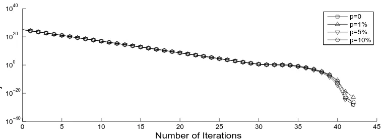
We start the investigation for simultaneously determining the time-dependent un-knowns a1 and a2 for exact and noisy input data, i.e., for the cases p ∈ {0,1,5,10}% of

noise. Figure 1 presents the objective function (40), as a function of the number of itera-tions. From this figure one can notice that a rapid convergence is achieved in 42 iteraitera-tions. The objective function (40) converges to a very small minimum value ofO(10−28_).

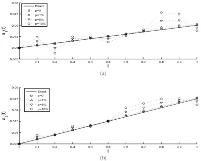
Figure 2 shows the unknown reconstructions fora1(t) anda2(t) for various noise levels.

As expected, the numerically obtained results become more stable and accurate as the percentage of noisepdecrease from 10% to 5% and then to 1%, seermse(a1) andrmse(a2)

in Table 1.

5.2

Example 2

The previous example has recovered the smooth time-dependent orthotropic conductivity components a1(t) and a2(t) given by (46). In this example we asses the performance of

the numerical method for reconstructing a non-smooth test case given by

a1(t) =

1 10

t−1₂

+₂₀1 , a2(t) =

1 10

t2 −1₂

+₂₀1 , t∈[0,1], (48)

and ugiven by (47). The input data φ, µi,j, νi,j,x0 and y0 are the same as in Example 1

but

f(x, y, t) = 1 5 t− 1 2 + 1 5 t2−

1 2 + 21

10, (49)

κ_{1(t) =} 3 5 t− 1 2 + 3

10, κ2(t) = 3 5

t2−

1 2 + 3

10. (50)

We take Mx = My = 10, N = 40 which, as in Example 1, together with the upper bound of 102 _{imposed ensure that the stability condition (30) is always satisfied during}

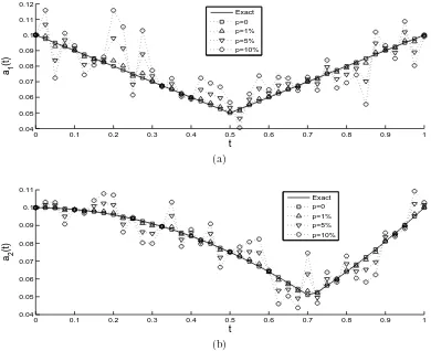
the iterative procedure. As we did in Example 1, Figures 3, 4 and Table 1 present the plots of objective function (40) as a function of the number of iterations, the numerically obtained reconstructions for the non-smooth coefficients and the rmse values (44) and (45) for Example 2, respectively. The same conclusions can be drawn about the stable reconstructions for the unknown coefficients.

6

Conclusions

The inverse problem concerning the simultaneous identification of the orthotropic ther-mal conductivity components a1(t) anda2(t) in a rectangular domain has been

theoret-ically and numertheoret-ically investigated. The unique solvability of the inverse problem has been established using Schauder’s fixed point theorem and the theory of Volterra integral equations of the second kind.

obtained. No regularization has been found necessary indicating that the inverse problem is in fact well-posed.

Acknowledgments

M.S. Hussein would like to thank the Ministry of Higher Education and Scientific Research for their financial support in this research. He would also like to thank the hospitality of Leeds University.

References

[1] Barans’ka, I.E. The inverse problem in a domain with free bound for an anisotropic equation of parabolic type, Naykovy Visnyk Chernivetskogo Universytetu Matem-atyka, 2008;374:13–28.

[2] Bereznytska, I.B. Inverse problem for a parabolic equation with non-local overdeter-mination condition. Math. Methods Phys.-Mech. Fields, 2001;44(1):54–62.

[3] Cannon, J.R. and Jones Jr., B.F. Determination of the diffusivity of an anisotropic medium, Int. J. Eng. Sci., 1963;1:457–460.

[4] Huang, L., Sun, X., Liu, Y. and Cen, Z. Parameter identification for two-dimensional orthotropic material bodies by the boundary element method, Eng. Anal. Boundary Elements, 2004;28:109–121.

[5] Hussein, M.S. and Lesnic, D. and Ivanchov, M.I. Identification of a heterogeneous orthotropic conductivity in a rectangular domain,Int. J. Novel Ideas: Mathematics, (accepted).

[6] Hussein, M.S., Lesnic, D., Ivanchov, M.I. and Snitko, H.A., Multiple time-dependent coefficient identification thermal problems with a free boundary, Appl. Num. Math., 2016; 99:24–50.

[7] Ivanchov, N.I. Some inverse problems for the heat equation with nonlocal boundary condition. Ukr. Math. J., 1993; 45(8):1066–1071.

[8] Ivanchov, M.I. On an inverse problem of heat conduction with nonlocal overdetermi-nation condition.Visnyk L’vivskogo Universytetu, Ser. Mech.-Mat., 1994;40:12–15.

[9] Ivanchov, M.I. Inverse Problems for Equations of Parabolic Type, VNTL Publishers, Liviv, Ukraine, 2003.

[10] Kinash, N. Inverse problem for the parabolic equation with nonlocal overdetermina-tion condioverdetermina-tion. Bukovynsky Math. J., 2015; 3(1):64–73.

[11] Knowles, I. and Yan, A. The recovery of an anisotropic conductivity in groundwater modelling, Appl. Anal., 2002; 81:1347–1365.

[13] Morton, K.W. and Mayers, D.F. Numerical Solution of Partial Differential Equa-tions: An Introduction, Cambridge University Press, Cambridge, 2005.

[14] Sawaf, B., Ozisik, M.N. and Jarny, Y. An inverse analysis to estimate linearly tem-perature dependent thermal conductivity components and heat capacity of an or-thotropic medium, Int. J. Heat Mass Transfer, 1995;38:3005–3010.

[15] Uhlmann, G. Developments in inverse problems since Calder´on’s foundational paper, In: Harmonic Analysis and Partial Differential Equations, University of Chicago Press, Chicago, IL, USA, pp. 295–345, 1999.

0 5 10 15 20 25 30 35 40 45

10−40 10−20 100 1020 1040

Number of Iterations

Objective function

p=0 p=1% p=5% p=10%

0 0.1 0.2 0.3 0.4 0.5 0.6 0.7 0.8 0.9 1 0.005

0.01 0.015 0.02 0.025 0.03

t

a 1

(t)

Exact p=0 p=1% p=5% p=10%

(a)

0 0.1 0.2 0.3 0.4 0.5 0.6 0.7 0.8 0.9 1 0.005

0.01 0.015 0.02 0.025 0.03

t

a 2

(t)

Exact p=0 p=1% p=5% p=10%

(b)

Figure 2: The exact solution (—) and numerical solutions for various noise levels p ∈

{0,1,5,10_}% for (a)a₁(t) and (b) a₂(t), for Example 1.

0 1 2 3 4 5 6

10−30 10−20 10−10 100 1010

Number of Iterations

Objective function

p=0 p=1% p=5% p=10%

0 0.1 0.2 0.3 0.4 0.5 0.6 0.7 0.8 0.9 1 0.04

0.05 0.06 0.07 0.08 0.09 0.1 0.11 0.12

t a 1

(t)

Exact p=0 p=1% p=5% p=10%

(a)

0 0.1 0.2 0.3 0.4 0.5 0.6 0.7 0.8 0.9 1

0.04 0.05 0.06 0.07 0.08 0.09 0.1 0.11

t a 2

(t)

Exact p=0 p=1% p=5% p=10%

(b)

Figure 4: The exact solution (—) and numerical solutions for various noise levels p ∈

{0,1,5,10_}% for (a)a₁(t) and (b) a₂(t), for Example 2.

Table 1: Thermse values (44) and (45) for various noise levels p_{∈ {}0,1,5,10_}%.

Example 1 p= 0 p= 1% p= 5% p= 10% rmse(a1) 2.6E-4 5.1E-4 0.0020 0.0038

rmse(a2) 2.9E-4 4.5E-4 0.0014 0.0026

Example 2 p= 0 p= 1% p= 5% p= 10% rmse(a1) 2.9E-16 0.0014 0.0070 0.0140