Mesh
.
White Rose Research Online URL for this paper:
http://eprints.whiterose.ac.uk/126358/
Version: Accepted Version
Article:
Gully, Amelia Jane orcid.org/0000-0002-8600-121X, Daffern, Helena
orcid.org/0000-0001-5838-0120 and Murphy, Damian Thomas
orcid.org/0000-0002-6676-9459 (2017) Diphthong Synthesis Using the Dynamic 3D Digital
Waveguide Mesh. IEEE/ACM Transactions on Audio, Speech, and Language Processing.
pp. 243-255. ISSN 2329-9290
https://doi.org/10.1109/TASLP.2017.2774921
[email protected] https://eprints.whiterose.ac.uk/ Reuse
Items deposited in White Rose Research Online are protected by copyright, with all rights reserved unless indicated otherwise. They may be downloaded and/or printed for private study, or other acts as permitted by national copyright laws. The publisher or other rights holders may allow further reproduction and re-use of the full text version. This is indicated by the licence information on the White Rose Research Online record for the item.
Takedown
If you consider content in White Rose Research Online to be in breach of UK law, please notify us by
Diphthong Synthesis using the
Dynamic 3D Digital Waveguide Mesh
Amelia J. Gully,
Member, IEEE,
Helena Daffern, and Damian T. Murphy
Abstract—Articulatory speech synthesis has the potential to offer more natural sounding synthetic speech than established concatenative or parametric synthesis methods. Time-domain acoustic models are particularly suited to the dynamic nature of the speech signal, and recent work has demonstrated the potential of dynamic vocal tract models that accurately reproduce the vocal tract geometry. This paper presents a dynamic 3D digital waveguide mesh (DWM) vocal tract model, capable of movement to produce diphthongs. The technique is compared to existing dynamic 2D and static 3D DWM models, for both monophthongs and diphthongs. The results indicate that the proposed model provides improved formant accuracy over existing DWM vocal tract models. Furthermore, the computational requirements of the proposed method are significantly lower than those of comparable dynamic simulation techniques. This work represents another step toward a fully-functional articulatory vocal tract model which will lead to more natural speech synthesis systems for use across society.
Index Terms—Speech synthesis, digital waveguide mesh, nu-merical acoustic modeling, diphthongs.
I. INTRODUCTION
T
HE current generation of speech synthesizers produce speech that is generally intelligible but still clearly iden-tifiable as less natural than recorded speech [1], and rarely, if ever, mistaken for a real human voice. This may be at-tributed in part to the techniques used: commercially available synthetic speech is generated largely by unit selection synthe-sis [2], while text-to-speech research currently focuses upon statistical parametric approaches making use of hidden Markov models [3] and more recently, deep neural networks [4]. These aim to reproduce the speech signal, rather than modeling the vocal system, and so are inherently limited by the database of recorded speech information and rules that they use. Even though transforms have been developed to model different speakers, emotions and personalities [5], creating perfectly natural-sounding speech with these methods would require an infinitely large database as well as the ability to model non-linguistic natural features such as laughter, coughing, breathing, and other human mannerisms. This is problematic for patients that use assistive technologies to speak, and may lead to self-esteem and stigmatization issues [6]; furthermore, there is evidence to show that signal-based approaches to speech synthesis affect the intelligibility for some vulnerable listeners [1], [7].Manuscript received Month Day, Year; revised Month Day, Year. The work of A. J. Gully was supported by an EPSRC Doctoral Training Partnership, number EP/K503216/1.
The authors are with the Audio Lab, Department of Electronics, Uni-versity of York, York, YO10 5DD, UK (e-mail: [email protected], [email protected], [email protected]).
A speech systembased approach, articulatory speech syn-thesis, has significant potential to overcome the problems de-scribed above and to generate truly natural-sounding synthetic speech [8]. Modern articulatory synthesis systems based on transmission lines, such as [9], offer a reasonable amount of detail and intuitive control mechanisms, facilitating the study of linguistic features such as coarticulation [10]. However, the transmission line approach, and analogous methods such as the Kelly-Lochbaum articulatory synthesiser [11] and improve-ments [12], [13], simplify the geometry of the vocal tract into a series of axisymmetric tube sections, reducing much of the detail of the vocal tract. This loss of detail has been shown to affect frequencies above 4 kHz [14], which are of vital perceptual importance for the judgment of naturalness [15].
In order to retain the detailed 3D geometry of the vocal tract, magnetic resonance imaging (MRI) data of the vocal tract shape may be used in conjunction with numerical acoustic modeling techniques, to accurately model the physics of the vocal system. One such technique is the finite element method (FEM), and the time-domain FEM approach outlined in [16] allows the model to change shape over time, facilitating the synthesis of dynamic speech sounds. This method has recently been shown to generate accurate diphthongs [17]. However, the computational load associated with FEM models of the vocal tract is extremely high; for example, the vocal tract models in [18] require 70–80 hours of computation time for 20 ms of output. Alternative modeling methods that use regular domain discretization schemes have lower, but still significant, computational requirements, and these have also been used to model the vocal tract. Such approaches include the finite-difference time domain (FDTD) method [19], [20], the digital waveguide mesh (DWM) [21], and the transmission line matrix (TLM) method [22], the latter two of which are equivalent to one another and, under certain circumstances, to the FDTD method [23]. FDTD, DWM, and TLM models have been shown to reproduce the vocal tract transfer function (VTTF) more accurately than the simplified axisymmetric tube models described above, but at present their shape cannot be changed during synthesis, making them suitable only for the reproduction of static speech units such as held vowels.
speech. A fixed simulation volume prevents errors associated with moving domain boundaries. The method is tested using the eight English diphthongs to illustrate its potential to deliver natural sounding synthetic speech. Although this model is not yet capable of running in real time, it offers comparable results to the FEM approach for significantly lower computational cost.
The remainder of this paper is laid out as follows: Section II introduces the DWM method, with the application of the DWM to vocal tract modeling described in Section III. In Sections IV and V, static and dynamic applications of the pro-posed technique are presented and discussed. Data associated with this study are detailed in Section VI, and conclusions and avenues for further study presented in Section VII.
II. DIGITALWAVEGUIDEMESHSYNTHESIS
The digital waveguide mesh (DWM) is a numerical acoustic modeling technique for solving the scalar wave equation that was first introduced in [24]. Under certain conditions the DWM is equivalent to a finite difference time domain (FDTD) scheme operating at the Courant limit [23], [25], and is also known as the transmission line matrix (TLM) method. Despite a higher computational load than the FDTD method, the DWM method is used for the present work as its stability is well-established [26] and the implementation of a heterogeneous simulation domain is simple and intuitive. The suitability of the DWM and equivalent TLM methods for vocal tract simulation has been established in e.g. [21], [22]. The scalar wave equation is sufficient to describe the production of vowels [27], which is the focus of this paper.
The DWM consists of a grid of regularly spaced scatter-ing junctions connected by unit digital waveguide elements. The scattering junctions may be connected in any regular arrangement in any number of dimensions. In this study, a 3D rectilinear mesh is used. This is conceptually the simplest mesh topology, and though it has been shown to introduce significant dispersion error at frequencies above one tenth of the temporal sampling frequency fs [28], the value for fs used in this study is sufficiently high that this does not affect the audio range. Acoustic variables, commonly pressure or velocity, are propagated throughout the mesh in the form of traveling-wave variables, or W-variables. The scattering of values throughout the mesh is governed by the admittances of the connecting waveguides.
A. The DWM algorithm
The DWM algorithm consists of three stages, which must be completed at every time step,n, for every scattering junction,
J, in the mesh [29]. The first stage is the scattering of W -variables:
pJ(n) =
2PNi=1Yip+J,i(n) PN
i=1Yi
(1)
wherepJ(n)is the acoustic pressure at scattering junctionJ at time stepn,Yi is the acoustic admittance of the waveguide connecting junction J to junction i, p+J,i(n) is the pressure incident at junction J from junction i at time step n, and
N is the number of waveguides connecting junction J to its neighbors: for a 3D rectilinear mesh, N= 6.
The second stage is to calculate the outgoing pressure from a junction into its neighboring waveguides. This uses a rearranged form of the junction continuity expression such that:
p−
J,i(n) =pJ(n)−p+J,i(n) (2)
where p−
J,i(n) is the pressure output by junction J into the waveguide connecting it to junctioni.
The final stage is to introduce a unit delay between adjacent scattering junctions, so the outgoing wave variable from one junction becomes the input to a neighboring junction at the next time step:
p+J,i(n) =p−
i,J(n−1) (3)
B. Heterogeneous and dynamic modeling
As described in [13], the boundaries of a DWM simulation domain cannot be simply moved during a simulation without introducing discontinuities in the output signal. Making a DWM model dynamic therefore requires a fixed-size grid, within which the admittance values may vary. This results in a heterogeneous simulation domain. To make the model dynamic, the admittance values are made to vary with time, replacing Yi in (1) with Yi(n). With suitable matrices of values Y(n) for each waveguide connection direction, any time-varying combination of acoustic media can be modeled. The derivation of stability conditions for such a time-varying model is an open problem, but in the current work the rate of change ofY(n)is slow compared to the system sampling frequency and the system remains stable.
The use of a heterogeneous simulation method allows the scattering behavior within the simulation domain to be com-pletely determined by the matrix of admittance values, known as the admittance map. With sufficient spatial resolution, com-plicated three-dimensional shapes such as the vocal tract can be modeled by accurately mapping the locations of the airway and the surrounding tissue to admittances in the domain. The process for doing this is described in Section III-C. Although this modeling technique has not commonly been used in room acoustics or vocal tract modeling, it has a long history of use in the field of geophysics, e.g. [30], where acoustic simulations are performed with local propagation parameters, such as wave speed, varying point-by-point throughout a fixed-size simulation domain.
C. Boundary conditions
The heterogeneous DWM domain has an effective shape governed by the admittance map. However, behavior at the edges of the domain, denoted ΓD, must also be specified. A number of boundary fomulations exist for the DWM, with one of the most common being the locally reacting wall (LRW) method [31]. The LRW is implemented at the domain boundary, ΓD, located at the external edges of a 3D domain. A normalized admittance parameter,G, specifies the reflection properties of the boundary.
(a) (b)
(c) (d)
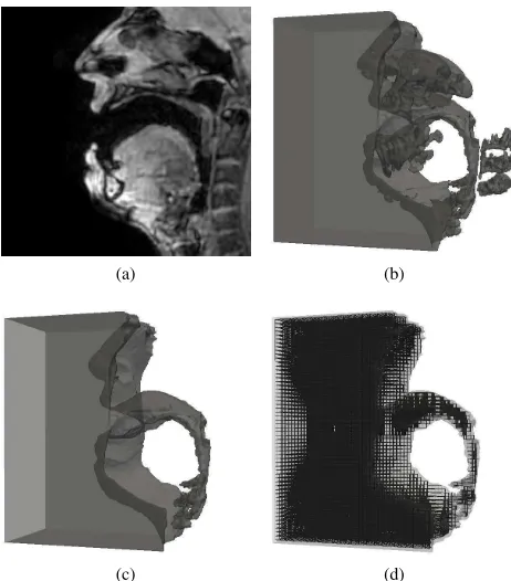
Fig. 1. Standardization procedure for vowel /a/, from (a) MRI data (mid-sagittal slice shown), through (b) segmentation procedure (illustrating leakage of the segmentation volume into surrounding tissues), (c) hand-corrected segmentation data, and (d) associated rectilinear grid, calculated using a sampling frequency of 400 kHz.
behavior of the admittance map causes the majority of energy to be reflected back into the vocal tract. Any energy reaching the edges of the domain should, intuitively, not reflect back into the domain. Likewise, under the assumption of free-field conditions outside the mouth, radiated pressure should not be reflected at the edges of the domain. Therefore, the boundaries of the model should be as close to anechoic as possible.
The proposed model therefore makes use of LRW bound-aries with an approximately anechoic condition achieved by setting the normalized admittance parameter G to one, not-ing that this boundary condition is known not to perfectly reproduce ideal anechoic behavior [31]. The behavior of the boundaries is explored further in Section III-B and found to be sufficiently accurate for the current study.
III. DWM VOCALTRACTMODELING
This section describes the application of the dynamic DWM method to 3D models of the vocal tract based on magnetic resonance imaging (MRI) data of the vocal tract geometry.
A. Data Acquisition and Pre-Processing
In order to create a DWM model of the vocal tract, it is necessary to obtain vocal tract shape information. The most accurate data for this purpose comes from MRI data of the upper airway. In this study, the MRI corpus collected in [21] is used. This corpus consists of 11 vowels and several other phonemes for five trained speakers, each of which was held for
16 s while a 3D scan procedure was completed. The images are 512×512×80 anisotropic grayscale images, resampled from
2 mm isotropic images. In order to focus machine resolution on the vocal tract, the images only extend to approximately 4 cm either side of the midsagittal plane, and hence do not capture the subject’s entire head.
In addition to the MRI data, anechoic audio recordings of the same utterances were collected immediately before and after the MRI scans. These recordings were made in MRI-like conditions with the participant in a supine position and MRI machine noise played back over headphones to disturb au-ditory feedback, recreating the vocalization conditions within the MRI scanner. The full details of the collection process are presented in [21]. This study makes use of the vocal tract information for a single adult male subject, with the nasal tract omitted due to poor resolution in that part of the image. A vocal-tract-only model is sufficient for vowel synthesis but it is acknowledged that the model must be extended to include a nasal tract if it is to be capable of synthesizing the full range of phonemes in the future.
In this study we consider the eight English diphthongs: /eI/ as inday, /aI/ as inhigh, /OI/ as inboy, /e@/ as infair, /@U/ as in show, /I@/ as in near, /U@/ as in jury, and /aU/ as in now. Therefore, it is necessary to use MRI data for the phonemes /e/, /a/, /I/, /O/, /@/, and /U/. Once collected, the MRI data must be pre-processed in order to generate a rectilinear grid of points representing the vocal tract volume. A complete overview of this process is illustrated in Fig. 1.
The MRI scan data, an example of which is shown in Fig. 1(a), must first be analyzed to obtain the vocal tract shape. The software ITK-Snap [32] is used for this purpose, which performs user-guided active contour segmentation based on image contrast, and is specifically designed for anatomical structures. However, as there is no difference in contrast between air and hard structures such as bone and teeth in MRI scan data, the segmentation volume initially includes the teeth as part of the airway1. MRI segmentation algorithms are also
prone to leakage into surrounding tissue areas, so the initial results of the segmentation often look similar to Fig. 1(b), with the teeth, several vertebrae, and parts of the jaw bone and nasal cavity included as part of the vocal tract airway. The resulting volume must be inspected, and any erroneous sections removed by hand, giving the final edited volume as shown in Fig. 1(c). This volume includes small side branches to the vocal tract, notably: the piriform fossae, two small cavities located at the bottom of the pharynx, either side of the esophageal entrance; and the epiglottic valleculae, two further cavities on the anterior pharyngeal wall at the base of the epiglottis.
The segmentation volume is allowed to expand beyond the mouth and out to the limits of the MRI image, resulting in a roughly cuboid volume of air coupled with the internal vocal tract airway. This air volume allows for realistic radiation behavior at the lips. The edges of this cuboid are modeled with approximately anechoic boundaries as described in
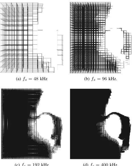
[image:4.612.57.288.63.326.2](a)fs= 48kHz (b)fs= 96kHz.
[image:5.612.58.292.64.356.2](c)fs= 192kHz (d)fs= 400kHz.
Fig. 2. Grids for phoneme /I/ with different sampling frequencies, with spatial step size given by (4).
tion II-C.
After the segmentation is complete, it must then be con-verted into a rectilinear 3D mesh. This step makes use of the custom code described in [21] to fit a Cartesian grid into the stencil created by the segmentation data. This process may be completed at any temporal sampling frequency, and generates a series of points which represent the physical locations of scattering junctions in the digital waveguide mesh algorithm (see Section II), as illustrated in Fig. 1(d).
Choosing the temporal sampling frequency for the model requires careful consideration. The equivalent physical length of unit waveguides in the DWM is related to the sampling frequency by the following relationship:
l=c
√
D fs
(4)
where c is the speed of sound in the medium, D is the dimensionality of the system (for the proposed model,D= 3), and fs is the sampling frequency. As a result, increasing
fs reduces the waveguide length l, providing better spatial resolution but also generating more scattering junctions in the volume. This results in increased computational complexity since calculations must be performed for every scattering junction at every time step. There is an additional lower limit on sampling frequency for vocal tract data, illustrated in Fig. 2, due to the small dimensions involved. If the sampling frequency is too low, the mesh becomes discontinuous, as seen in Fig. 2(a) and 2(b). In the heterogeneous DWM, this means that no channel of lower admittance—as detailed in Section
(a) Case 1: whole head with ex-tended radiation volume
(b) Case 2: whole head with lim-ited radiation volume
(c) Case 3: front hemisphere only (d) Case 4: MRI extent only Fig. 3. Volume matrices for phoneme /a/ with different radiation volumes. Each volume matrix contains a 3D Cartesian grid of points whose extent is indicated by the surrounding boxes; black points represent scattering junction locations that exist within the head tissue. Axis units are scattering junction indeces inx,yandzdirections.
III-C—would exist to connect the front and back vocal tract cavities. Even at 192 kHz (Fig. 2(c)), there are parts of the vocal tract represented by a single layer of scattering junction locations, equivalent to a physical depth of zero. As a result, the sampling frequency chosen for this study is 400 kHz, as illustrated in Fig. 2(d), giving a spatial resolution of approx-imately 1.52 mm. At this grid resolution there are at least two scattering junctions, and hence at least one waveguide, in every dimension at a constriction for all the phonemes under study. This grid spacing therefore provides an appropriate trade-off between spatial resolution and computational expense for the synthesis of diphthongs. It should be noted that the constrictions in the vocal tract during consonant articulation may be narrower than those for vowels, and therefore the grid resolution must be carefully considered when the model is extended to include consonants.
B. Mesh alignment and extent
[image:5.612.317.549.70.306.2]Fig. 4. Location and definition of domain boundaries and vocal tract wall for simulations. Midsagittal slice through a 3D volume representing vowel /O/ is shown.
extends approximately 4 cm either side of the midsagittal plane so the remaining head geometry is unknown. This technique provides an appropriate head volume while retaining subject-specific geometry such as the nose and particularly the lips, known to be essential for accurate vocal tract acoustics [27].
The radiation volume is a critical aspect of vocal tract simulations, and accurate synthesis requires this volume to be taken into account [18], [27]. However, too large a simulation domain results in high computational cost for potentially small increases in accuracy. Therefore, simulations were performed to determine how much the radiation volume and head tissue can be constrained without introducing significant errors in the VTTF. Four cases were investigated, as illustrated in Fig. 3. In every case, the bottom of the simulation domain was fixed at a location approximately 1 cm below the larynx position for the articulation of /O/, which had the lowest larynx position of all the articulations studied. In Case 1, the entire head was considered with 10 cm air surrounding it; Case 2 also features the entire head but with 1 cm air to the sides and back and 3 cm in front; Case 3 is similar to Case 2 but with the back of the head removed, up to 1 cm behind the back of the phayrngeal wall; and Case 4 consists of the extent of the original MRI image with 3 cm air in front, extending approximately 4 cm either side of the midsagittal plane, and up to the top of the nose.
Figure 4 illustrates a midsagittal slice through an example simulation domain corresponding to Case 4. The external boundaryΓDmay be further split into domain edges occuring within air, ΓDA, and domain edges within head tissue,ΓDT. An anechoic LRW boundary is implemented on ΓDA and
ΓDT, as described in Section II-C. The vocal tract wallΓW is not implemented as a domain boundary in the proposed model; instead the difference in admittance that occurs atΓW causes reflection of sound waves back into the vocal tract airway. The process of creating an admittance map is described in the next section.
The VTTF, H(f), was calculated as follows [27]:
H(f) = Pout(f)
Uin(f) (5)
Fig. 5. Vocal tract transfer functions for phoneme /a/ in each radiation volume case. An artificial 50 dB offset has been added between VTTFs for clarity of illustration.
wherePout(f)and Uin(f) are the Fourier transforms of the output acoustic pressure signal and the input volume velocity signal, respectively. Following [19], a Gaussian pulse, gp(t), was used as the volume velocity source, calculated as follows:
gp(t) =e−[(∆tn−T)/0.29T] 2
(6)
where∆t= 1/fs,T= 0.646/f0andf0= 20kHz, providing sufficient excitation across the entire audible frequency range of 0–20 kHz. For clarity, and direct comparison with other simulations such as [19] and [27], only the frequency range 0–10 kHz is displayed in Figs. 5–7. This range is sufficient to describe speech intelligibility, and much of the informaton relating to naturalness [15]. However, full-bandwidth VTTF plots are available in the accompanying data (see Section VI). The resulting VTTFs for the vowel /a/ are presented in Fig. 5, and similar results are obtained for the other phonemes under study. It is apparent from Fig. 5 that in general, the VT-TFs are very similar for each of the four cases. Cases 1 and 2 in particular exhibit almost identical VTTFs, with less than 1 dB difference in the entire range 0-20 kHz. Some small errors are introduced for Cases 3 and 4, primarily affecting the depth of spectral dips. However, Case 4 introduces further errors, with a 3 dB difference in the first two formant magnitudes compared to Case 1, and a large deviation below 500 Hz. For this reason, volume matrices cropped according to Case 3 are used throughout the remainder of this study, as they provide an appropriate trade-off between model accuracy and simulation domain size, and hence computation time.
The similarity of Cases 1 and 2 is particularly significant as it suggests that the LRW anechoic boundary implementation used on ΓD—which, for a receiver located outside the vocal tract at a close, on-axis position, is much closer to the receiver position in Case 2 than Case 1—does not have a significant effect on the simulated transfer functions. It can therefore be assumed that the LRW produces boundaries that are sufficiently close to anechoic for the purposes of the current study.
C. Admittance Map Construction
[image:6.612.316.561.57.184.2]The volume matrices described in Section III-B consist of a regular arrangement of scattering junction locations, with values of either one (when the junction is located within the airway) or zero (when the junction is located within the tissue of the head). However, in a DWM it is the waveguides— the links betweenscattering junctions—that have a physically meaningful admittance; the scattering junctions represent the infinitesimally small points at which these waveguides meet. Therefore, in order to generate an admittance matrix it is necessary to perform a complete interrogation of the connec-tions between scattering juncconnec-tions to determine the appropriate admittances.
If two neighboring volume matrix elements are both located within the airway, the waveguide connecting the junctions is assigned the admittance of air, Y0 = 1/Z0, where the impedance of air is related to the speed of sound in air, c0 and the density of air ρ0 as follows: Z0 = ρ0c0. Following previous studies [17], [27], the values c0 = 350 m s−1 and
ρ0 = 1.14 kg m−3 are used, giving Z0 = 399 Pa s m−3. If two neighboring volume matrix elements are both located within the head tissue, the connecting waveguides are assigned the admittance of the tissue forming the vocal tract wall,
Yw= 1/Zwwherecw= 1500 m s−1andρw= 1000 kg m−3, hence Zw = 1.5×10⁶ Pa s m−3. This value is based on measured properties of tissue and has been used in a previous study [20]. Lower values, such as Zw = 83666 Pa s m−3, have been used in other studies (e.g. [17], [27]), but were found to result in less accurate formant values when used in the proposed method. This may be due to the fact that the proposed model uses a single impedance value for the whole head, so it must take into account higher impedance structures such as bone. In the final case, where neighboring volume matrix elements span the air/tissue interface Γw, the connecting waveguide is assigned the admittance Yw. This gives a tissue boundary location accurate to within the length of one unit waveguide, which at 400 kHz is approximately 1.52 mm according to (4). The MRI corpus is resampled from a 2 mm isotropic image, so this level of spatial resolution is appropriate given the data available.
The process described above is repeated for every volume matrix element and connection direction. For a 3D rectilin-ear mesh, this results in six admittance matrices, which for ease of conceptualization are termed Ynorth,Ysouth,Yeast,
Ywest,Yf rontandYback. The matrices are constructed such that Ynorth(x, y, z) represents the admittance in the waveg-uide directly north of the junction with index (x, y, z), and
Ysouth(x, y, z) represents the admittance in the waveguide directly south of this junction, such thatYnorth(x+ 1, y, z) =
Ysouth(x, y, z). Once these admittance maps have been popu-lated, moving between vocal tract shapes is simply a matter of interpolating between maps over the duration of a simulation, as discussed in Section V-A.
[image:7.612.315.562.57.183.2]Once the admittance maps are complete, the scattering behavior within the model is established. The final step is to select suitable source and receiver positions for the simulation.
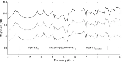
Fig. 6. Vocal tract transfer functions for phoneme /O/ with local and global source positions. An artificial 50 dB offset has been added between VTTFs for clarity of illustration.
D. Source and receiver positions
During vowel production, a source signal is generated at the larynx, and speech is output at the lips. In simulations of the vocal tract, the aim is to replicate this behavior. The larynx moves between vowel articulations, so an ideal simulated source would also move within the simulation domain.
Most finite element vocal tract models (e.g. [27]) apply a source signal across the entire cross-sectional area of the glottal opening, known as the glottal boundary ΓG. As the simulation domain changes shape, so does the location of
ΓG and hence the source position. In DWM simulations, the source signal is inserted at one or more scattering junction locations. Changing the junction(s) at which a signal is input during the course of the simulation introduces audible artifacts in DWM simulations, and as such is beyond the scope of this work. Instead, a single scattering junction, pexcitation is selected as the excitation point for all the phonemes under study.
Selecting an excitation point requires careful consideration, as the larynx height within the mesh varies depending on the phoneme, with /a/ having the highest larynx position and /O/ having the lowest in the phonemes under study. To ensure that
pexcitation is not located below the laryngeal opening for any of the phonemes, it is placed at a level corresponding to the highest larynx location, namely that of /a/, and is therefore also within the airway for the other five phonemes under study.
To investigate the error caused by locating the source at
TABLE I
PERCENTAGE ERROR IN FORMANT FREQUENCY FOR SIMULATIONS,COMPARED TO RECORDED SPEECH(M.A.IS MEAN ABSOLUTE ERROR)
2DD-DWM 3DS-DWM 3DD-DWM
Vowel F1 F2 F3 F4 F5 M.A. F1 F2 F3 F4 F5 M.A. F1 F2 F3 F4 F5 M.A.
a -23.8 -12.7 -6.5 -1.9 -9.2 10.8 -9.8 -19.8 -14.1 -1.2 -9.8 10.9 16.6 -8.8 -3.0 0.5 -9.0 7.6
e -3.5 -14.7 -9.7 -9.7 -7.7 9.1 6.6 -17.3 -11.9 -13.2 -15.6 12.9 16.6 -7.6 -1.4 -0.7 4.3 6.1
I -2.7 -53.9 -14.1 -7.8 -2.9 16.3 -16.6 -11.4 -8.3 -15.0 -19.4 14.1 -5.5 0.7 6.9 -5.1 -7.1 5.0 O 27.4 67.9 3.5 17.9 12.1 25.8 30.0 9.4 -12.8 -8.3 -22.8 16.7 46.1 21.9 -5.3 9.6 -7.9 18.2 U -4.6 61.4 -2.3 -2.9 -2.1 14.7 -7.2 -5.9 -24.1 -17.8 -19.5 14.9 8.9 9.1 -11.9 -4.4 -7.1 8.3 @ -0.3 9.0 -7.0 1.4 4.1 4.4 -2.4 -14.1 -15.9 -13.9 -18.7 13.0 10.4 -1.7 -6.5 -0.8 -5.3 4.9 M.A. 10.4 36.6 7.2 6.9 6.4 13.5 12.1 13.0 14.5 11.6 17.6 13.8 17.4 8.3 5.8 3.5 6.8 8.4
formant magnitudes are also within 6 dB of those generated with the input applied on the scattering junctions representing
ΓG—which is assumed to be the most accurate case—in the region below 9 kHz. Between 9–12 kHz (see associated data files for full-bandwidth VTTF figures), there are large differences in magnitude caused by the altered source location, although the formant frequencies remain accurate. Between 12 kHz and 20 kHz, the error remains under 6 dB. This is considered sufficiently accurate for the current model, given the additional sources of error in the simulated VTTF such as the absence of a nasal cavity. As these simulations used the phoneme with the greatest difference in height between the actual larynx and pexcitation, errors in the VTTF related to source position are smaller for the other phonemes under study. The VTTF generated using a single point on ΓG as the input location also results in the correct formant frequencies and less than 2 dB error across the majority of the audio bandwidth.
In addition to pexcitation, a receiver position preceiver is also selected, as a single point at an on-axis position level with the tip of the nose, similar to a real, close microphone position. As the nose is one of the points used to align the vocal tract data, this position is considered to be suitable for all the phonemes under study and approximates the position of the microphone during the comparison audio recordings.
Once admittance maps have been generated and suitable source and receiver positions selected, simulations may be performed.
IV. MONOPHTHONGSYNTHESIS
The proposed method must be compared to recorded voice data and existing DWM synthesis techniques in order to confirm its accuracy. This section describes the procedures that were undertaken to this end, using static vowel articulations.
A. Procedure
The proposed method is compared to two existing DWM vocal tract simulation techniques: the dynamic 2D model [13], henceforth referred to as the2DD-DWMmodel, and the static 3D model [21], henceforth called the3DS-DWMmodel. These are compared with the proposed dynamic 3D model, labeled the 3DD-DWM model. For the current comparison, fixed vowel articulations are used, so all the simulations may be considered ‘static’. Simulations are performed using the 3DD-DWM procedure outlined in Section III for each of the six
monophthongs required to make up the English diphthongs: /e/, /a/, /I/, /O/, /@/, and /U/.
A comparison 3DS-DWM simulation is performed follow-ing [21], based on the same volume matrix as the 3DD-DWM simulation. The 3DS-DWM is a homogeneous simulation that takes place only on the scattering junctions representing the airway, with an approximately anechoic LRW boundary set up on ΓDA, and a reflecting boundary set up on ΓW with a reflection coefficient of 0.99. This value was found to provide a suitable formant bandwidth in agreement with [21].
The final simulation method used in the comparisons is the 2DD-DWM method. This method simplifies the vocal tract by treating it as a concatenation of cylindrical tubes with cross-sectional areas obtained from the vocal tract geometry. In order to create 2DD-DWM models that are comparable to the 3DD-DWM and 3DS-DWM models, the same 3D MRI data was used. This data was converted to cross-sectional area data following the iterative bisection procedure described in [34]. A heterogeneous 2D DWM was set up according to the method in [13], with the cross-sectional area mapped to admittance across the width of the DWM, following a raised-cosine relationship. The resulting model has a channel of high admittance along the center of the mesh, with lower admittance at the domain edges that varies with distance from the glottis, in proportion to the cross-sectional area at the same distance from the glottis. As a result, a one-dimensional model of the vocal tract is mapped to a 2D DWM, providing a means of simulating cross-tract modes and other acoustic effects that result in improved simulation accuracy over one-dimensional simulation methods [13]. The same sampling frequency of 400 kHz was used for the 2DD-DWM simulations, resulting in a spatial resolution of 1.24 mm according to (4). The 2DD-DWM model does not include provision for radiation at the lips, nor any energy lost at the glottis; instead a specific reflection coefficient is set at either end of the mesh to approximate this behavior. Following the recommendation of [35], this lip reflection coefficient is set to -0.9, the glottal reflection coefficient to 0.97, and the reflection coefficient at mesh boundaries to 0.92.
(a) /a/
(b) /e/
(c) /@/
(d) /I/
(e) /O/
[image:9.612.55.298.59.556.2](f) /U/
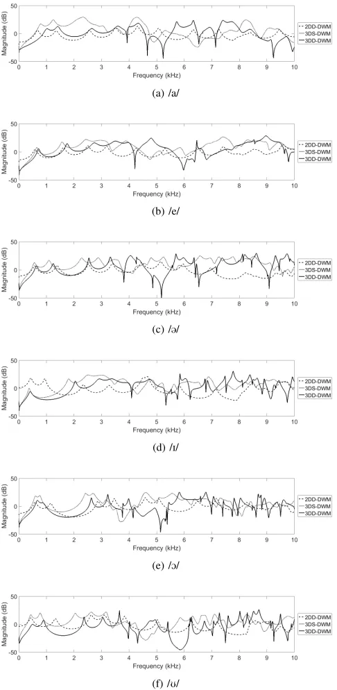
Fig. 7. VTTFs for monophthongs simulated using 2DD-DWM, 3DS-DWM and 3DD-DWM methods.
be used to assess the performance of the simulations.
B. Results and Discussion
The percentage errors of the first five formants relative to corresponding recorded speech are presented for each simulation method in Table I, and the calculated vocal tract transfer functions (VTTFs) are presented in Fig. 7.
It is apparent from Table I that simulation accuracy varies between vowels for all simulation methods. In particular, simulation of the vowel /O/ results in large errors for every method, suggesting that the subject may not have been consistent in their articulation between the MRI scan and
audio recording. The simulation errors vary even for the other five vowels, raising the important point that the accuracy of 3D vocal tract models may be vowel-specific. It should also be noted that some error may have been introduced during the process of segmenting the MRI data to obtain the vocal tract airway shape. It is worth noting that very few 3D vocal tract models in the literature compare their output to recorded speech, perhaps due to the lack of suitable speech data from the same subject used for MRI scans. The only available comparisons appear to be from [20] (FDTD), [21] (DWM) and [36] (FEM). Simulations in [20] produce a mean absolute error of 6.07%, for the vowel /a/ only, using a 3D FDTD vocal tract model—although the origin of the speech data used for comparison is not clear—which is of comparable magnitude to the mean error of 7.6% obtained for /a/ using the proposed 3DD-DWM method. The 3DS-DWM method in [21] provides formant errors in Hz rather than percentages, but these are also of comparable magnitude to the formant errors observed for the 3DS-DWM simulation in the present study. Finally, [36] indicates highly vowel-dependent results, but across the four vowels studied the mean absolute error is 12.3%.
The value of the first formant—except in the case of /O/ noted above—is generally underestimated by the 2DD-DWM and 3DS-DWM methods, whereas in the proposed 3DD-DWM method, F1 is generally overestimated by a significant margin. The frequency of the first formant is known to increase when yielding walls are taken into account [37], which may help to explain why the 3DD-DWM model, where sound is allowed to propagate through the vocal tract walls, results in a higher F1 value than the other simulations, which feature effectively hard walls with simple losses. The values of F1 for the proposed model remain higher than for the recordings, indicating that the value chosen for the wall impedance in Section III-C may still be too low; however, higher values were found to introduce more error in the higher formant frequencies. This result suggests that frequency-dependent impedances are necessary for accurate formant reproduction, in agreement with previous studies [38]. This issue is expected to be addressed in future versions of the model, which will incorporate filters to approximate frequency-dependent behavior at the vocal tract walls. In the meantime, audition indicates that the high F1 values do not affect vowel identification.
errors in these higher formants and the 2DD-DWM method in particular shows errors of greater than 50% for F2 for some vowels, which may affect intelligibility. The improvement of the 3DD-DWM simulation over the 2DD-DWM simulation is expected, as the 2DD-DWM makes a number of simplifying assumptions such as considering the vocal tract to be a straight, axisymmetric tube. Additionally, it has been shown in [39] and [40] that a number of tuning steps are required to produce accurate formation locations and bandwidths from 2D vocal tract simulations. The improvement of the 3DD-DWM model over the 3DS-DWM model appears to be, at least in part, due to the modeling of the vocal tract walls as having some depth through which sound can propagate, as in the real vocal tract. It has been shown that the “staircase” boundary approximation inherent in Cartesian meshes introduces significant errors in acoustic simulations [41]. This is most relevant to the 3DS-DWM simulation where the boundary is applied at the edge of the vocal tract, so interpolation of non-Cartesian boundary locations such as the immersed boundary method [42] or finite-volume boundary layers [41] may improve formant accuracy in this case.
The simulated VTTFs, illustrated in Fig. 7, provide more detail about the three simulation methods. It is immediately apparent that, in addition to the differences in formant frequencies described in Table I, the relative formant magnitudes, and often the formant bandwidths, differ with simulation method. Relative formant magnitudes are important in the perception of naturalness [27], but without a VTTF of the real vocal tract for comparison—planned for the next stage of this research—the accuracy of formant magnitudes are difficult to assess.
One clear feature of the 3DD-DWM VTTFs (see Fig. 5 and 6) are large spectral dips, occurring at different frequencies depending on the vowel. Similar spectral dips—occurring at different frequencies and with different depths—are visible in Fig. 7 in the VTTFs generated using the 3DS-DWM method. By systematic occlusion of the vocal tract side branches, individually and in combination, the spectral dips are identified as the contribution of the piriform fossae and epiglottic valleculae. Although [19] found the acoustic effects of the epiglottic valleculae to be small, for this subject they are found to contribute significantly to the VTTF, both individually and in combination with the piriform fossae. As the dips are associated with vocal tract side branches, which are not modeled in the 2DD-DWM simulation, they are not present in the VTTFs for the 2D simulation method.
Using the vowel /@/, which has a range of spectral dips visible in the VTTF, as an example, the contribution of the different side branches to the 3DD-DWM VTTF can be seen. Spectral dips occurring at 3.8 kHz and 4.8 kHz are due to the left and right piriform fossae respectively, indicating a difference in their size. The epiglottic valleculae are responsible for the spectral dips at 6.5 kHz and 9 kHz. Finally, it is the piriform fossae and epiglottic valleculae interacting with one another that produces the large spectral minimum at 5.2 kHz; none of the side branches account for this dip on their own.
The 3DS-DWM simulation features spectral dips for the same reasons, but they are generally lower in frequency and shallower in depth than those seen for the 3DD-DWM VTTFs. For example, for /@/, the dips corresponding to the left and right piriform fossae occur at 3.1 kHz and 4.1 kHz respectively. These differences appear to be a result of the boundary implementation on ΓW in the 3DS-DWM simulation, whereas in the 3DD-DWM model, a waveguide with the admittance of tissue spans this interface, effectively reducing the size of the vocal tract by up to one waveguide length (≈ 1.52 mm) in each direction. It is difficult to
determine which of the simulated VTTFs is the most correct, although the 3DD-DWM simulation produces piriform fossae dips closer to the expected range of 4–5 kHz [43]. This effective reduction in cavity size between the 3DS-DWM and 3DD-DWM simulations may also contribute to differences in formant locations between the two simulation methods.
Audition of the accompanying audio files (see Section VI) permits further insight into the simulation accuracy. In general, the 2DD-DWM simulations sound intelligible but buzzy, and as might be predicted from the large errors in F2, the simulated /I/ sounds more like /U/, and /O/ sounds more like /2/. The 3DS-DWM and 3DD-DWM simulations present a definite improvement over 2DD-DWM, although neither might be considered as sounding natural. Each of the 3D simulations has a different character, making it difficult to compare the two methods in terms of simulation accuracy, but both present intelligible vowel sounds.
It is important to note that the results presented in this section may be specific to the MRI subject used, and further studies must consider additional participants, with a range of ages and sexes, before general conclusions can be made.
V. DIPHTHONGSYNTHESIS
Dynamic models have a further advantage in that they are capable of moving between vocal tract shapes and hence simu-lating dynamic speech. In this section, results of a comparison between the dynamic 2D model, dynamic 3D model, and recorded diphthongs are presented.
A. Procedure
The procedure for the diphthong simulations is similar to that of the monophthongs in Section IV-A, but the 3DS-DWM model is excluded from the comparison as it is not capable of producing dynamic sounds. In both the 2DD-DWM and 3DD-DWM simulations, admittance maps are generated representing the start and end points of the diphthongs—for example, /a/ and /I/ for the diphthong /aI/—and the admittance map used in the simulation is interpolated between the two over the duration of the simulation, following a half-wave sinusoid trajectory (the shape of a sine wave from −π/2 to
(a)
(b)
[image:11.612.319.558.55.460.2](c)
Fig. 8. Spectrograms for diphthong /OI/: (a) 2DD-DWM simulation, (b) 3DD-DWM simulation, and (c) recording.
As the simulations in this comparison are dynamic, a source signal is injected directly into the simulation domain at the source position detailed in Section III-D. An electrolaryngo-graph (Lx) signal is used for this purpose, which is a measure of vocal fold conductivity, and is inverted to provide a signal approximating the real glottal flow during an utterance [44]. The Lx data was recorded simultaneously with the benchmark audio recordings, and is used as the simulation input to provide the correct pitch contour and amplitude envelope associated with the recorded audio. The use of the recorded Lx source facilitates direct comparison between the simulations and the recordings.
B. Results and Discussion
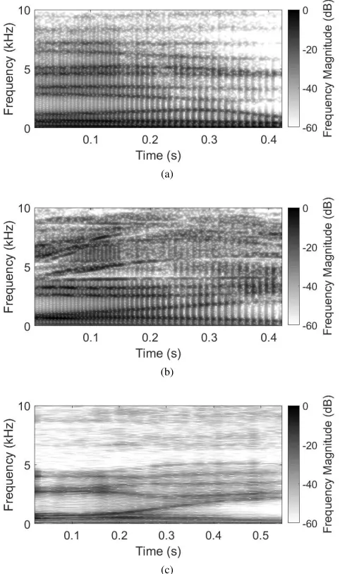
The spectrograms of the syntheized and recorded diphthongs /OI/ and /aU/ can be seen in Fig. 8 and Fig. 9 respectively. Spectrograms for all diphthongs under study are presented in the additional data described in Section VI. As is common for speech research, a pre-emphasis FIR filter,
(a)
(b)
(c)
Fig. 9. Spectrograms for diphthong /aU/: (a) 2DD-DWM simulation, (b) 3DD-DWM simulation, and (c) recording.
with coefficients [1 -0.97], has been applied to the recorded and synthesized speech data to more clearly illustrate the high frequency components.
It may be seen that although the 2DD-DWM simulations reproduce the lower formants with relative accuracy—apart from /I/ which was noted in the previous section to have an artificially low F2 value—above approximately 4 kHz additional spurious, closely-spaced formants are introduced due to simplification of the vocal tract geometry in the 2D simulation. This is consistent with the findings of the previous section. The dynamic 3D simulation more closely reproduces the number and frequencies of higher formants in the recorded data, due largely to the improved geometrical accuracy of detailed 3D simulations such as the inclusion of side branches.
[image:11.612.56.297.58.464.2]recorded speech data. This is consistent with the findings from [21]. This energy originates from the source Lx signal, which approximates the real vocal source but does not exactly reproduce it. The model currently contains no mechanism to reproduce the frequency-dependent damping within the vocal tract, which causes the reduction in high frequency energy visible in the spectrograms of recorded speech. This occurs due to viscous and thermal losses and other absorption phenomena, and may be approximated by the addition of a filter to the model. It should be noted, however, that similar high frequency energy is present in diphthongs simulated using the FEM method [17], indicating that the 3DD-DWM method produces comparable results.
Another issue that must be addressed in the dynamic 3D model is the matter of phoneme-specific transitions. As F2 in Fig. 8(a) illustrates, simulated formant transitions may not follow the same half-wavelength sinusoid shape used in the simulation. Furthermore, every articulation of a given diphthong will be different, even when uttered by the same speaker. It is also clear from the formant traces in Fig. 9(c) that articulations may be held fixed before and after a transition occurs. Clearly, a simple model such as a sinusoidal interpolation is insufficient for controlling the vocal tract model. Much work has been done on the subject of phoneme transitions in the context of transmission-line articulatory models (see, for example, [10] and references therein). The process of translating the control parameters of a highly simplified 1D vocal tract model into parameters suitable for control of a detailed 3D geometry presents a significant engineering challenge, but one which is essential to the generation of a suitable control system for the proposed model.
Audio data is also available for the dynamic simulations presented in this section. Upon audition, the 3DD-DWM simulations—while still subject to the high-frequency noise and transition limitations described above—sound significantly more natural than the 2DD-DWM simulations. Additionally, the phonemic content of the utterance is more clearly identifiable in 3D simulations. Both of these effects may be attributed to the considerably improved geometry of the 3D model over the 2D model. By reproducing vocal tract geometry more accurately, corresponding resonance and hence formant behavior is reproduced, leading to better vowel identification. The results are also consistent with the audio output of the FEM diphthong model [17]. Although the various limitations described throughout this paper mean that the 3DD-DWM model does not yet reproduce completely natural voice sounds, the results presented in this section indicate a significant increase in accuracy compared to previously available DWM models.
C. Implementation
The complexity of the proposed algorithm is presented in Table II. The primary computational expense is the large number of divisions required. The static 3D model explored in Section IV requires significantly fewer operations, as the
TABLE II
ALGORITHM COMPLEXITY OF DYNAMIC3D DWMSIMULATION IN TERMS OF ADDITION,MULTIPLICATION AND DIVISION OPERATIONS
For mesh sizeK×L×M, for timen= 1,2, . . .
+ × ÷
1. add input values topinput 1 – –
2. calculate junction pressurepJ 10KLM 7KLM KLM
3. calculate node outputsp−
J,i 6KLM – –
4. updatep+J,ivalues – – – 5. extract output sample – – – 6. update admittance maps 6KLM – – Total 22KLM+ 1 7KLM KLM
assumption of a homogeneous mesh eliminates divisions from step 2 and removes step 6 entirely, resulting in an overall requirement of9KLM+ 1additions and7KLM multiplica-tions per time step. In addition, the static model is a stationary system, and as such its impulse response is sufficient to describe its behavior: once this has been calculated, it may be convolved with any source. The dynamic model, however, cannot be completely defined in this way, and as such the simulation must be performed over the duration of every input, resulting in much higher computation times overall. A serial MATLAB implementation of the system requires processing times on the order of 13 hours to generate a second of output sound, which is still significantly faster than the 70–80 hours required to generate 20 ms of output using the FEM method in [18]. This speed can be further improved using parallel ar-chitectures and/or faster programming languages: for example, a parallel MATLAB implementation using an NVIDIA 1070 GPU reduces the processing time to approximately 3 hours per second of output. While the 2D dynamic model of [13] is capable of running in real time, this is only possible due to the highly simplified geometry and low sampling rate used in the study. In the case of the dynamic 3D model, the complexity is necessary in order to obtain both dynamic movement and improved naturalness in the output.
VI. DATA
The data used in this study has been made available at [45]. They consist of WAV-format audio files of recordings, all simulations, and Lx input files used for all monophthongs and diphthongs presented. In addition, full audio bandwidth figures for all monophthongs and diphthongs are presented, along with the MATLAB code used for their generation, and the 3D segmentation data for the 6 vocal tract shapes used.
VII. CONCLUSION
a significant increase in accuracy over existing 2D DWM models [13] for diphthong synthesis.
Future work will compare simulated vocal tract transfer functions to those measured from human subjects, in order to determine the frequency-dependent absorption characteristics of the vocal tract airway, and the influence of different tissue types within the vocal tract walls. A complete set of listening tests is also planned in order to determine the perceptual naturalness of the model, which is the ultimate measure of its success in synthesizing speech.
This work represents an important step towards the generation of a fully-functional articulatory model of the vocal tract which, in the future, may be able to operate in real time and produce natural sounding synthetic speech for implementation across society, in applications beyond the uses of current synthesis systems.
ACKNOWLEDGMENT
The authors would like to thank members of the Audio Lab at the Department of Electronics, University of York, and Pro-fessor David Howard, for support and helpful discussions, and Kat Young for providing the idealized head mesh. The authors also extend their thanks to the staff of York Neuroimaging Centre (YNiC) and the participants of the MRI data collection procedure. Author A. Gully is supported by a University of York EPSRC Doctoral Training Partnership.
REFERENCES
[1] S. J. Winters and D. B. Pisoni, “Perception and comprehension of speech synthesis,” inEncylopedia of Language and Linguistics, 2nd Edition, K. Brown, Ed. Oxford, UK: Elsevier Science, Ltd., 2006, pp. 31–49. [2] A. J. Hunt and A. W. Black, “Unit selection in a concatenative speech synthesis system using a large speech database,” inProc. Int. Conf. Acoust. Speech Signal Process., Atlanta, GA, 1996, pp. 373–376. [3] K. Tokuda, Y. Nankaku, T. Toda, H. Zen, J. Yamagishi, and K. Oura,
“Speech synthesis based on hidden Markov models,”Proc. IEEE, vol. 101, no. 5, pp. 1234–1252, May 2013.
[4] H. Zen, A. Senior, and M. Schuster, “Statistical parametric speech synthesis using deep neural networks,” inProc. Int. Conf. Acoust. Speech Signal Process., Vancouver, Canada, May 2013, pp. 7962–7966. [5] J. Yamagishi, B. Usabaev, S. King, O. Watts, J. Dines, J. Tian, Y. Guan,
R. Hu, K. Oura, Y. Wu, K. Tokuda, R. Karhila, and M. Kurimo, “Thousands of voices for HMM-based speech synthesis—analysis and application of TTS systems built on various ASR corpora,”IEEE Trans. Audio Speech Language Process., vol. 18, no. 5, pp. 984–1004, Jul. 2010.
[6] S. E. Stern, “Computer-synthesized speech and perceptions of the social influence of disabled users,”J. Lang. Soc. Psychol., vol. 27, no. 3, pp. 254–265, Sep. 2008.
[7] L. Blomert and H. Mitterer, “The fragile nature of the speech-perception deficit in dyslexia: natural vs. synthetic speech,”Brain Lang., vol. 89, no. 1, pp. 21–26, Apr. 2004.
[8] C. H. Shadle and R. I. Damper, “Prospects for articulatory synthesis: a position paper,” inProc. 4th ISCS Workshop Speech Synthesis, Blair Atholl, Scotland, 2001, pp. 121–126.
[9] P. Birkholz, D. Jack`el, and B. J. Kr¨oger, “Simulation of losses due to turbulence in the time-varying vocal system,”IEEE Trans. Audio Speech Language Process., vol. 15, no. 4, pp. 1218–1226, May 2007. [10] P. Birkholz, “Modeling consonant-vowel coarticulation for articulatory
speech synthesis,”PLOS One, vol. 8, no. 4, p. e60603, Apr. 2013. [11] J. L. Kelly and C. C. Lochbaum, “Speech synthesis,” inProc. 4th Int.
Congr. Acoust., Copenhagen, Denmark, Aug. 1962, pp. 1–4.
[12] V. V¨alim¨aki and M. Karjalainen, “Improving the Kelly-Lochbaum vocal tract model using conical tube sections and fractional delay filtering techniques,” inProc. Int. Conf. Spoken Language Process., Yokohama, Japan, 1994, pp. 615–618.
[13] J. Mullen, D. M. Howard, and D. T. Murphy, “Real-time dynamic articulations in the 2D waveguide mesh vocal tract model,”IEEE Trans. Audio Speech Language Process., vol. 15, no. 2, pp. 577–585, Feb. 2007. [14] R. Blandin, M. Arnela, R. Laboissi`ere, X. Pelorson, O. Guasch, A. V. Hirtum, and X. Laval, “Effects of higher order propagation modes in vocal tract like geometries,”J. Acoust. Soc. Am., vol. 137, no. 2, pp. 832–843, Feb. 2015.
[15] B. B. Monson, E. J. Hunter, A. J. Lotto, and B. H. Story, “The perceptual significance of high-frequency energy in the human voice,”
Front. Psychol., vol. 5, no. 587, pp. 1–11, Jun. 2014.
[16] O. Guasch, M. Arnela, R. Codina, and H. Espinoza, “A stabilized finite element method for the mixed wave equation in an ALE framework with application to diphthong production,”Acta Acust. united Ac., vol. 102, no. 1, pp. 94–106, Jan. 2016.
[17] M. Arnela, O. Guasch, S. Dabbaghchian, and O. Engwall, “Finite element generation of vowel sounds using dynamic complex three-dimensional vocal tracts,” inProc. 23rd Int. Congr. Sound Vib., Athens, Greece, Jul. 2016.
[18] M. Arnela, R. Blandin, S. Dabbaghchian, O. Guasch, F. Al´ıas, X. Pelor-son, A. V. Hirtum, and O. Engwall, “Influence of lips on the production of vowels based on finite element simulations and experiments,” J. Acoust. Soc. Am., vol. 139, no. 5, pp. 2852–2859, May 2016. [19] H. Takemoto, P. Mokhtari, and T. Kitamura, “Acoustic analysis of
the vocal tract during vowel production by finite-different time-domain method,”J. Acoust. Soc. Am, vol. 128, no. 6, pp. 3724–3738, Dec. 2010. [20] Y. Wang, H. Wang, J. Wei, and J. Dang, “Mandarin vowel synthesis based on 2D and 3D vocal tract model by finite-difference time-domain method,” inProc. APSIPA Annu. Summit Conf., Hollywood, CA, Dec. 2012.
[21] M. Speed, D. Murphy, and D. Howard, “Modeling the vocal tract transfer function using a 3D digital waveguide mesh,”IEEE Trans. Audio Speech Language Process., vol. 22, no. 2, pp. 453–464, Feb. 2014.
[22] A. S. Brand˜ao, E. Cataldo, and F. R. Leta, “On the apparent propagation speed in transmission line matrix uniform grid meshes,”J. Vib. Acoust., vol. 136, no. 6, Oct. 2014, 61013.
[23] M. Karjalainen and C. Erkut, “Digital waveguides versus finite differ-ence structures: equivaldiffer-ence and mixed modeling,”EURASIP J. Appl. Signal Process., vol. 2004, no. 7, pp. 978–989, Jun. 2004.
[24] S. A. V. Duyne and J. O. Smith, “Physical modeling with the 2D digital waveguide mesh,” in Proc. Int. Comput. Music Conf., Tokyo, Japan, 1993, pp. 40–47.
[25] D. T. Murphy and M. Beeson, “The KW-boundary hybrid digital waveguide mesh for room acoustics applications,”IEEE Trans. Audio Speech Language Process., vol. 15, no. 2, pp. 552–564, Feb. 2007. [26] S. Bilbao,Numerical Sound Synthesis: Finite Difference Schemes and
Simulation in Musical Acoustics. Chichester, UK: John Wiley and Sons Ltd., 2009.
[27] M. Arnela, O. Guasch, and F. Al´ıas, “Effects of head geometry simpli-fications on acoustic radiation of vowel sounds based on time-domain finite-element simulations,” J. Acoust. Soc. Am., vol. 134, no. 4, pp. 2946–2954, Oct. 2013.
[28] A. Southern, T. Lokki, and L. Savioja, “The perceptual effects of dispersion error on room acoustic model auralization,” inProc. Forum Acusticum, Aalborg, Denmark, 2011, pp. 1553–1558.
[29] D. Murphy, A. Kelloniemi, J. Mullen, and S. Shelley, “Acoustic mod-eling using the digital waveguide mesh,” IEEE Signal Process. Mag., vol. 24, no. 2, pp. 55–66, Mar. 2007.
[30] K. R. Kelly, R. W. Ward, S. Treitel, and R. M. Alford, “Synthetic seismograms: a finite-difference approach,”Geophysics, vol. 41, no. 1, pp. 2–27, 1976.
[31] K. Kowalczyk and M. V. Walstijn, “Formulation of locally reacting surfaces in FDTD/K-DWM modelling of acoustic spaces,”Acta Acustica united with Acustica, vol. 94, no. 6, pp. 891–906, Nov. 2008. [32] P. A. Yushkevich, J. Piven, H. C. Hazlett, R. G. Smith, S. Ho, J. C.
Gee, and G. Gerig, “User-guided 3D active contour segmentation of anatomical structures: significantly improved efficiency and reliability,”
Neuroimage, vol. 31, no. 3, pp. 1116–1128, Jul. 2006.
[33] H. Takemoto, T. Kitamura, H. Nishimoto, and K. Honda, “A method of tooth superimposition on MRI data for accurate measurement of vocal tract shape and dimensions,”Acoust. Sci. Tech., vol. 25, no. 6, pp. 468– 474, 2004.
[34] B. H. Story, I. R. Titze, and E. A. Hoffman, “Vocal tract area functions from magnetic resonance imaging,”J. Acoust. Soc. Am., vol. 100, no. 1, pp. 537–554, Jul. 1996.
increased model dimensionality,”IEEE Trans. Audio Speech Language Process., vol. 14, no. 3, pp. 964–971, May 2006.
[36] D. Aalto, A. Huhtala, A. Kivel a, J. Malinen, P. Palo, J. Saunavaara, and M. Vainio, “How far are vowel formants from computed vocal tract resonances?”arXiv:1208.5962v2 [math.DS], Oct. 2012.
[37] K. N. Stevens,Acoustic Phonetics. Cambridge, MA: The MIT Press, 1998.
[38] M. Fleischer, S. Pinkert, W. Mattheus, A. Mainka, and D. M urbe, “Formant frequencies and bandwidths of the vocal tract transfer function are affected by the mechanical impedance of the vocal tract wall,”
Biomech. Model. Mechanobiol., vol. 14, no. 4, pp. 719–733, 2015. [39] M. Arnela and O. Guasch, “Two-dimensional vocal tracts with
three-dimensional behavior in the numerical generation of vowels,”J. Acoust. Soc. Am., vol. 135, no. 1, pp. 369–379, Jan. 2014.
[40] ——, “Finite element synthesis of diphthongs using tuned two-dimensional vocal tracts,” IEEE/ACM Trans. Audio Speech Language Process., vol. 25, no. 10, pp. 2013–2023, Oct. 2017.
[41] S. Bilbao, B. Hamilton, J. Botts, and L. Savioja, “Finite volume time domain room acoustics simulation under general impedance bound-ary conditions,” IEEE/ACM Trans. Audio Speech Language Process., vol. 24, no. 1, pp. 161–173, Jan. 2016.
[42] J. Wei, W. Guan, D. Q. Hou, D. Pan, W. Lu, and J. Dang, “A new model for acoustic wave propagation and scattering in the vocal tract,” inProc. INTERSPEECH, San Francisco, CA, Sep. 2016.
[43] T. Kitamura, K. Honda, and H. Takemoto, “Individual variation of the hypopharyngeal cavities and its acoustic effects,” Acoust. Sci. Tech., vol. 26, no. 1, pp. 16–26, 2005.
[44] I. R. Titze, “Parameterization of the glottal area, glottal flow, and vocal fold contact area,”J. Acoust. Soc. Am., vol. 75, no. 2, pp. 570–580, Feb. 1984.
[45] A. Gully, 2016. [Online]. Available: tinyurl.com/h98peum
PLACE PHOTO HERE
Amelia J. Gully(M’12) received the B.Sc. (Hons.) degree in audio technology from the University of Salford, UK, in 2010 and the M.Sc. degree in dig-ital signal processing from the University of York, UK, in 2013. She is currently pursuing the Ph.D. degree in electronic engineering at the University of York, UK, studying dynamic physical modeling of the vocal tract. Her research interests include voice analysis and synthesis, numerical acoustic modeling, and assistive technologies.
PLACE PHOTO HERE
Helena Daffernreceived the BA (Hons.) degree in music, the M.A. degree in music, and the D.Phil. degree in music technology, all from the University of York, UK, in 2004, 2005, and 2009, respectively. She is currently a Lecturer in Music Technology in the Department of Electronic Engineering at the University of York. Her research focuses on voice science and acoustics, particularly singing perfor-mance, vocal pedagogy, choral singing and singing for health.
PLACE PHOTO HERE