Braid groups and quiver mutation

(1)

This is a repository copy of Braid groups and quiver mutation.

White Rose Research Online URL for this paper:

http://eprints.whiterose.ac.uk/113358/

Version: Accepted Version

Article:

Grant, J and Marsh, RJ orcid.org/0000-0002-4268-8937 (2017) Braid groups and quiver

mutation. Pacific Journal of Mathematics, 290 (1). pp. 77-116. ISSN 0030-8730

https://doi.org/10.2140/pjm.2017.290.77

© 2017 Mathematical Sciences Publishers. This is an author produced version of a paper

published in Pacific Journal of Mathematics. Uploaded in accordance with the publisher's

self-archiving policy.

[email protected] https://eprints.whiterose.ac.uk/ Reuse

Unless indicated otherwise, fulltext items are protected by copyright with all rights reserved. The copyright exception in section 29 of the Copyright, Designs and Patents Act 1988 allows the making of a single copy solely for the purpose of non-commercial research or private study within the limits of fair dealing. The publisher or other rights-holder may allow further reproduction and re-use of this version - refer to the White Rose Research Online record for this item. Where records identify the publisher as the copyright holder, users can verify any specific terms of use on the publisher’s website.

Takedown

If you consider content in White Rose Research Online to be in breach of UK law, please notify us by

(2)

Braid groups and quiver mutation

Joseph Grant and Robert J. Marsh

Abstract

We describe presentations of braid groups of type ADE and show how these presentations are compatible with mutation of quivers. In typesA andD these presentations can be under-stood geometrically using triangulated surfaces. We then give a categorical interpretation of the presentations, with the new generators acting as spherical twists at simple modules on derived categories of Ginzburg dg-algebras of quivers with potential.

Keywords: mutation, braid groups, cluster algebras, Ginzburg dg algebra, spherical twist

2010 Mathematics Subject Classification. Primary: 13F60, 16G20, 20F36; Secondary: 16E35, 16E45, 18E30.

1 Introduction

Braid groups are fundamental objects in mathematics. Although they are of a topological and geo-metric nature, they have an algebraic interpretation: a simple presentation by generators and relations which is just based on adjacency of integers [Ar]. This can be encoded in a line graph, and from there one can generalize to define a group from any finite graph, known as the Artin braid group.

(3)

quotient of a corresponding Artin braid group in a natural way. In particular, the symmetric group onnletters is a quotient of the classical braid group onnstrands. Coxeter groups naturally split into two distinct classes: those of finite type, corresponding to the Dynkin diagrams of type ADE, and those of infinite type. Although all Artin braid groups are infinite, the Artin braid groups of Dynkin type have a different character to those not of Dynkin type, and are known as Artin groups of ‘finite type’.

This dichotomy also arises in another area of mathematics which has generated a lot of interest in the recent years: cluster algebras. In this theory, there is a notion of finite-type cluster algebras, which again correspond to the Dynkin diagrams [FZ2]. Cluster algebras are specified by a directed graph, known as a quiver, together with other information. A key ingredient in the definition is the notion of mutation, which changes the arrows in a quiver in a non-obvious manner which generalizes reflection at a source or sink. Barot and Marsh [BM] have given new presentations of Coxeter groups of finite type based on quivers obtained from Dynkin diagrams under finite sequences of mutations. Our first result generalizes this to braid groups:

Theorem A. (Theorem 2.12) Let Q be a quiver, with vertices 1, 2, ... ,n, obtained from a Dynkin

quiver by a finite sequence of mutations. Let BQ be the group with generators s1,s2, ... ,sn, subject

to the relations:

(a) sisj=sjsi if there is no arrow between i and j (in either direction);

(b) sisjsi =sjsisj if there is an arrow between i and j (in either direction);

(c) si1si2· · ·sinsi1· · ·sin−2 = si2si3· · ·sinsi1· · ·sin−1 =· · ·, whenever i1 → i2 → · · · → in → i1 is a

chordless cycle in Q.

Then BQ is isomorphic to the Artin braid group of the same Dynkin type as Q.

We prove our result via isomorphisms between abstractly defined groups, which can be thought of as mutations of groups, even though the resulting groups are isomorphic. The Artin group presentations we obtain induce presentations of the corresponding Coxeter groups which are distinct from those in [BM]; we also give a compatibility result which shows the relationship between the two presentations. Why have we chosen to use presentations which don’t agree with the earlier work? This is explained in the following two sections of the paper, as we now detail.

Certain cluster algebras can be understood using pictures. A (tagged) triangulation of a Riemann surface with marked points on its boundary defines a quiver [FZ1, FoSTh]; see also [CCS]. Then mutation of the quiver has a natural interpretation in terms of swapping one diagonal of a given quadrilateral for the other. So these cluster algebras have a topological interpretation. In particular, such descriptions are available for the infinite families of Dynkin type. A natural question is: can we understand the generators above, and the isomorphisms corresponding to mutations, in terms of the geometry of the surface? The answer is yes:

Theorem B. (Theorem 3.6) Let∆be a Dynkin diagram of type An or type Dn. In the former case,

let (X,M) be a disk with n+ 3 marked points on its boundary. In the latter case, let(X,M)be a disk with n marked points on its boundary and one marked point in its interior, taken to be a cone point of order2 (so X is an orbifold in this case).

(4)

is an isomorphism between the subgroup HT of the braid group generated by theσi and the group BQ defined above, takingσi to si.

Furthermore, in type An, HT coincides with the braid group of (X,M), while in type Dn, HT is of index two in the braid group of (X,M).

As well as the original combinatorial and commutative algebraic approach to cluster algebras, and the geometric approach described above, there is a third approach which has proved very power-ful: the representation theoretic approach [BMRRT, CCS]. This approach uses finite dimensional (noncommutative) algebras and ideas from categorification to better understand cluster algebras, and has received intense study. Braid groups also appear in representation theory and categorifica-tion [RZ, ST]: in many important situacategorifica-tions there are accategorifica-tions of braid groups on derived categories via spherical twists. One example of this is given by certain derived categories of differential graded algebras [Gin, KY] which are known to cover the categories appearing in the representation theoretic approach to cluster algebras [Am]. One might hope that these categorical braid group actions are related to our presentations of braid groups, and we show that this is indeed the case.

First, we make a connection between the categorical and the geometric situations. The relevant differential graded algebras are defined by use of a quiver together with a formal sum of cycles in that quiver known as a potential [Gin]. Mutation of quivers of potential has been defined [DWZ] and, in the situations where our cluster algebra comes from a Riemann surface, the mutation of potentials also has a geometric interpretation [LF09]. Relying heavily on results of Labardini-Fragoso [LF09, LF12], we observe that the potential defined on mutation-Dynkin quivers according to the geometric procedure is equivalent to the ‘obvious’ potential that one might guess (Proposition 4.4). So, while the potential is important, it is in fact entirely determined by the quiver in types A and D. Note that this result could also be proved relatively easily via a direct calculation.

Next we show that we do indeed obtain an action of the groupsBQ (defined using mutation-Dynkin quivers) on derived categories of Ginzburg differential graded algebras in which the generators act via spherical twists. After setting up all the technical machinery correctly, the main difficulty in proving this is to check that the mutation procedure for the groups BQ, which relates the group associated to a quiver to the group associated to a mutated quiver, actually lifts to the categorical setting as a natural isomorphism of functors. We do this, using important results of Keller and Yang [KY]. From here, we can use the earlier theory developed here to show that the generators si of finite type Artin braid groups from Theorem A can be viewed as derived autoequivalences:

Theorem C. (Theorem 4.16) Let(Q,W)be a mutation-Dynkin quiver with potential of type ADE ,

and let ΓQ,W be the corresponding Ginzburg differential graded algebra. Let Dfd(ΓQ,W) denote the full subcategory of the derived categoryD(ΓQ,W)on objects with finite-dimensional total homology. Then there is a group homomorphism

BQ →Aut Dfd(ΓQ,W) si7→Fi

sending the group generator associated to the vertex i of Q to the spherical twist Fi at the simple ΓQ,W-module Si.

(5)

typeD. In [Nag,§2.2], K. Nagao refers to an action of the mapping class group of a marked surface on the derived category of a Ginzburg dg-algebra associated to a triangulation.

Since we released the first draft of this article, the preprint [HHLP] has appeared, where the authors give a presentation (different from the one given here) of the Artin braid group for each diagram of finite type (in the cluster-theoretic sense). This includes the non-simply-laced cases (not considered here) but does not include a topological or categorical interpretation.

2 Presentations of braid groups

2.1 Braid groups

Let ∆ be a graph ofADE Dynkin type, i.e., ∆ is a graph of typeAn forn≥1,Dnforn≥4,E6,E7,

or E8.

TypeAn: •1 •2 •3 n−• 1 •n

TypeDn: • 1

• 2

• 3

• 4

• n−1

• n

In particular, ∆ has no double edges or cycles. Let I be the set of vertices of ∆. We can associate a group B∆ to ∆, which we call the braid group of ∆. It has a distinguished set of generators

S∆ = {si}i∈I, and the relations depend on whether or not two vertices are connected by an edge. They are as follows:

(i) sisj=sjsi if •i •j ;

(ii) sisjsi =sjsisj if •i •j ;

If ∆ is of typeAn then we recover the “usual” braid group, sometimes denotedBn+1. Its generators

can be visualized as follows:

si = •

1 _•2 _•i i+ 1_•

•

n n+ 1_•

•

1 •2 •i i+ 1• •n n+ 1•

and the relations of type (i) record the fact that crossings of far-apart adjacent pairs of strings commute, while relations of type (ii) record a Reidemeister 3 move.

If we also impose the relation that s2

(6)

2.2 Mutation of quivers

A quiver is just a directed graph. Throughout this article we will only work with quivers with finitely many vertices and finitely many arrows that have no loops or oriented 2-cycles. For a given quiver Q, we again denote its set of vertices byI.

There is a procedure to obtain one quiver from another, called quiver mutation, due to Fomin and Zelevinsky [FZ1,§4]. FixQ and letk ∈I. Then we obtain the mutated quiverµk(Q) as follows:

(i) for each pair of arrowsi→k →j throughk, add a formal compositei→j;

(ii) reverse the orientation of all arrows incident withk;

(iii) remove a maximal set of 2-cycles (we may have created 2-cycles in the previous two steps).

It is a basic but important observation that quiver mutation does not change the set of vertices. One can also check that mutation is an involution.

We call a cycle in an unoriented graph (or in the underlying unoriented graph of a quiver) chordless if the full subgraph on the vertices of the cycle contains no edges which are not part of the cycle. We call a quiverDynkinif its underlying unoriented graph is a Dynkin graph of typeADE, and mutation-Dynkin if it can be obtained by mutating a Dynkin quiver finitely many times. By a theorem of Fomin and Zelevinsky [FZ2, Thm. 1.4], there are only finitely many quivers that can be obtained by mutating a given Dynkin quiver.

The following fact will be useful to us.

Proposition 2.1(Fomin-Zelevinsky). In any mutation-Dynkin quiver, there are no double arrows and

all chordless cycles are oriented.

Proof: By [FZ2, Theorem 1.8], the entries in the corresponding exchange matrixBsatisfy|BxyByx| ≤ 3 for all x,y (known as being 2-finite). Hence there cannot be any double arrows in the quiver.

Now letQ be a mutation-Dynkin quiver andC a chordless cycle inQ. Then, sinceQ is 2-finite, so is C. By [FZ2, Proposition 9.7],C must be an oriented cycle. 2

2.3 Groups from quivers

LetQ be a mutation-Dynkin quiver.

Definition 2.2. From the quiver Q with vertex set I, we define the group BQ as follows: it has a

distinguished generating setSQ={si}i∈I and the relations given by:

(i) sisj=sjsi if •i •j ;

(7)

(iii) if we have an oriented chordlessn-cycle

1 //2

n

OO

. ..

oo

then

s1s2...sns1s2...sn−2=s2s3...sns1...sn−1

=· · ·

=sns1s2...sns1s2...sn−3

Remark 2.3. If Q is a Dynkin quiver, then BQ is (isomorphic to) the Artin braid group of the

corresponding Dynkin type.

This presentation is symmetric but not minimal:

Lemma 2.4. For each single chordless n-cycle, in the presence of the relations of type (i) and (ii),

any one of the relations of type (iii) implies all the others.

Proof: It is enough to show that if the relation

s1s2· · ·sns1s2· · ·sn−2=s2s3· · ·sns1s2· · ·sn−1 (1)

holds then

s1s2· · ·sns1s2· · ·sn−2=s3s4· · ·sns1s2· · ·sn.

So, we assume that (1) holds. Then we have:

s2−1s1s2· · ·sns1s2· · ·sn−2sn=s3· · ·sns1s2· · ·sn−1sn.

The left hand side can be rewritten, using relations of type (i) and (ii), as:

s2−1s1s2· · ·sns1s2· · ·sn−2sn=s1s2s1−1s3· · ·sns1s2· · ·sn−2sn

=s1s2s3· · ·sn−1s1−1sns1s2· · ·sn−2sn

=s1s2· · ·sn−1sns1sn−1s2· · ·sn−2sn

=s1s2· · ·sns1s2· · ·sn−2,

and the result follows. 2

Though the relations look different, by taking an appropriate quotient we can obtain the groups defined by Barot and Marsh [BM] directly:

Lemma 2.5. If we also impose the relations s2

i = 1 for all i ∈ I , then the group BQ becomes isomorphic to the groupΓU(Q) defined in [BM, Section 3], where U(Q)is the underlying graph of Q.

(8)

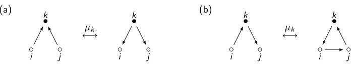
(a)

◦

i ◦j

•

k

µk

◦

i ◦j

•

k (b)

◦

i ◦j

•

k

µk

◦

i ◦j

•

[image:8.612.132.481.90.159.2]

k

Figure 1: Mutation of a quiver of mutation Dynkin type.

We need to show that, in the presence of relations (i), (ii), ands2

i = 1 for alli∈I, our extra relation (iii) holds if and only if the relation

(s1s2...sn−1snsn−1...s2)2= 1

and its rotations hold for eachn-cycle 1→2→ · · · →n→1. By symmetry, it is enough to check that the relation above is equivalent tos1s2...sns1s2...sn−2=s2s3...sns1...sn−1.

Using that si=s−1

i , we see that our our relation is equivalent to

s1s2...sns1s2...sn−2sn−1sn−2...s1sn...s3s2= 1.

Multiplying out the Barot-Marsh relation, we see that it is equivalent to

s1s2...sn−1snsn−1...s2s1s2...sn−1snsn−1...s2= 1.

Cancelling out n terms on the left and n−1 terms on the right of these two expressions, it just remains to show that

s1s2...sn−2sn−1sn−2...s2s1=sn−1sn−2...s2s1s2...sn−2sn−1.

As there is an arrowi→i+ 1 for eachiand the cycle is chordless, the symmetric group onnletters maps onto the subgroup generated by s1, ... ,sn−1 with the transposition which swaps i and i+ 1

being sent tosi. It is easy to see that the corresponding relation holds in the symmetric group, with both sides of the equation representing the transposition which swaps 1 and n. 2

We will justify our choice of relations in Remark 4.19.

2.4 Mutation of groups

Let BQ be the group associated to the mutation-Dynkin quiver Q, as above, and let k be a vertex of Q. Denote µk(Q) byQ′_{. Our aim in this section is to show that} _BQ _{is isomorphic to} _BQ

′. We

will do this by using a group homomorphismϕk :BQ →BQ′ defined using a formula which lifts the

formula used in [BM,§5].

The following lemma follows from results in [FZ2] (see [BM, §2]).

Lemma 2.6. Let Q be a quiver of mutation-Dynkin type, and fix a vertex k of Q. Suppose that

k has two neighbouring vertices. Then the possibilities for the induced subquiver of Q containing vertex k and its neighbours are shown in Figure 1. The effect of mutation is shown in each case.

(9)

Lemma 2.7. Let Q be a quiver of mutation-Dynkin type, and fix a vertex k of Q. Let C be an oriented cycle in Q. Then C is one of the following. In each case we indicate what happens locally under mutation at k.

(a)

◦

i ◦j

•

k

C

µk

◦

i ◦j

•

k (b)

◦

i1 ◦ir

•

k

◦

i2

◦

◦ir₋1

◦

C

µk

◦

i1 ◦ir

•

k

◦

i2

◦

◦ir₋1

◦ (c)

◦

i1 ◦ir

•

k

◦

i2

◦

◦ir₋1

◦

C

µk

◦

i1 ◦ir

•

k

◦

i2

◦

◦ir₋1

◦

(d) An oriented cycle containing exactly one neighbour of k. Mutation at k reverses the arrow between k and its neighbour in C .

(e) An oriented cycle containing no neighbours of k. Mutation at k does not affect C .

Recall that BQ is defined using generatorssi fori ∈I. We denote the corresponding generating set forBQ′ byti,i∈I. LetFQ be the free group on the generatorssi fori∈I.

Definition 2.8. Letϕk :FQ →BQ′ be the group homomorphism defined by

ϕk(si) =

(

tktit−1

k ifi→k inQ; ti otherwise.

Proposition 2.9. The group homomorphism ϕk induces a group homomorphism (which we also

denote byϕk) from BQ to BQ′.

Proof: Let us writeesi = ϕk(si). We must show that the elementsesi in BQ′ satisfy the defining

relations of BQ. Note that the ti satisfy the defining relations forBQ′.

Firstly, we check the relations (ii) for an arrow incident withk. Suppose that there is an arrowi→k. We have the following, using the fact that titkti =tktitk:

esi_esk_esi=tktitktit_k−1 =tk2titkt

−1

k =t

2

kti.

Also,

e

sk_esi_esk =t_k2tktit_k−1tk =t_k2ti.

So

(10)

If there is an arrowi←k, then we have

esieskesi =titkti =tktitk =eskesiesk.

Next, we consider relations (i) and (ii) for all other arrows in Q. Relations of this kind involving pairs of vertices which are not neighbours ofk follow immediately from the corresponding relations in BQ. If only one of the vertices in the relation is a neighbour of k, the relation again follows immediately since tk commutes with any generator corresponding to a vertex not incident withk in Q′ _{(equivalently, in}_Q_{). So we only need to consider the case where both of the vertices in the pair} is incident with k and we can use Lemma 2.6.

Going in either direction in part (a) of Lemma 2.6, the relation_esi_esj =_esj_esi follows from the relation titj=tjti inBQ′, so we consider part (b), firstly from left to right. The cycle inQ′ gives the relation

tkti =tjtktitjt_k−1t_j−1. Also applying the relationt_k−1t_j−1t_k−1=t_j−1t_k−1t_j−1, we obtain

esi_esj=tktit_k−1tj

=tjtktitjt_k−1t_j−1t_k−1tj

=tjtktit−1

k =esjesi.

Going from right to left in part (b), we have, using tjtktj=tktjtk,titj =tjti andtitkti =tktitk,

e

sj_esi_esj =tktjt−1

k titktjt −1

k =t_j−1tktjtit_j−1tktj

=t_j−1tktitktj

=t−1

j titktitj =tit_j−1tktjti

=titktjt_k−1ti =_esi_esj_esi.

Next, we have to check that the _esi satisfy the relations of type (iii) for Q, so we need to consider each the types of cycle described in Lemma 2.7. By Lemma 2.4, it is enough to check that, for any given cycle inQ, one of the relations in (iii) holds.

For part (a), we have

esk_esi_esj_esk =tktitktjt−1

k tk =tktitktj,

while

e

siesjeskesi =titktjt_k−1tkti =titktjti =titktitj,

(11)

For part (b) we have, applying a relation for the cycle in Q′ _{in the fourth step:}

e

si1esi2· · ·esiresi1esi2· · ·esir−2 =tkti1t

−1

k ti2· · ·tirtkti1t

−1

k ti2· · ·tir−2

=t_i−₁1tkti1ti2· · ·tirtkti1t

−1

k ti2· · ·tir−2

=t_i−₁1tkti1ti2· · ·tirtkti1ti2· · ·tir−2t

−1

k =t_i−₁1ti1ti2· · ·tirtkti1ti2· · ·tir−2tir−1t

−1

k =ti2· · ·tirtkti1t

−1

k ti2· · ·tir−2tir−1

=esi2· · ·esiresi1esi2· · ·esir−2esir−1.

For part (c), we have, applying a relation for the cycle in Q′ _{in the fourth step:}

esi1esi2· · ·esir−1esireskesi1· · ·esir−1=ti1ti2· · ·tir−1tktirt

−1

k tkti1· · ·tir−1

=ti1ti2· · ·tir−1tktirti1· · ·tir−1

=ti1tkti2· · ·tir−1tirti1· · ·tir−1

=ti1tkti1ti2· · ·tir−1tirti1· · ·tir−2

=tkti1tkti2· · ·tir−1tirti1· · ·tir−2

=tkti1ti2· · ·tir−1tktirt

−1

k tkti1· · ·tir−2

=_esk_esi1esi2· · ·esir−1esireskesi1· · ·esir−2,

and we are done. 2

Theorem 2.10. ϕk :BQ →BQ′ is a group isomorphism.

Proof: As mutation is an involution, we can consider the composition

ϕk :BQ ϕk

→BQ′ →ϕk BQ.

Fix some i ∈ I. Note that mutation atk does not change whether i and k are connected in the quiver: it just swaps the direction of any arrow that may exist betweeni andk. So if we havei→k then si 7→tktit−1

k 7→sksis −1

k . If we have i ←k then si 7→ti 7→sksis −1

k . And if there is no arrow between i andk then si 7→ti 7→si. But in this case si and sk commute, so si =sksis−1

k . Hence in every case ϕk(si) =sksis−1

k , soϕk is just a conjugation map and thereforeϕk :BQ →BQ′ is an

isomorphism. 2

Remark 2.11. The inverse ofϕk is the group isomorphismϕ−_k1:BQ′

∼

→BQ defined by

ϕ−_k1(ti) =

(

s_k−1sisk if i→k in Q; si otherwise.

Noting Remark 2.3, we have the following:

Theorem 2.12. If Q is a mutation-Dynkin quiver of type∆then BQ ∼=B∆.

3 Topological interpretation of the generators

3.1 Braid groups

(12)

group B∆ of the same Dynkin type. In other words,BQ gives a presentation ofB∆. In this section

we give a geometric interpretation of this presentation.

We associate an oriented Riemann surfaceS (with boundary) together with marked pointsMto ∆, as follows. If ∆ =An, we takeS to be a disk withn−3 marked points on its boundary, as in [FZ1, FZ2]. If ∆ = Dn, we take S to be a disk with one marked point in its interior and n marked points on its boundary, as in [FoSTh, Sch]. In each case, it was shown that every quiver of the corresponding mutation type arises from a triangulation of (S,M) (tagged, in the type Dn case) in the following way. We follow [FoSTh], in a generality great enough to cover both cases (noting that there is at most one interior marked point).

A (simple) arc in (S,M) is a curve in S (considered up to isotopy) whose endpoints are marked points inMand which does not have any self-crossing points, except possibly at its endpoints. Apart from these endpoints, it must be disjoint fromM and the boundary ofS, and it must not cut out an unpunctured one- or two-sided polygon.

Two arcs are said to be compatible if they are non-crossing in the interior of S. A maximal set of compatible arcs is a triangulation.

Atagged arc in (S,M) is an arc which does not cut out a once-punctured monogon; each of its ends is tagged, either plain or notched. Plain tags are omitted, while notched tags are displayed using the bow-tie symbol ⊲⊳. An end incident with a boundary marked point is always tagged plain. Two tagged arcsα,β arecompatible if

(i) the untagged arcs underlyingαandβ are compatible, and

(ii) if the untagged versions ofαandβ are different but share an endpoint, then the corresponding ends ofαandβ are tagged in the same way.

A tagged triangulation T of (S,M) is a maximal collection of tagged arcs in (S,M). Note that if none of the marked points inMlies in the interior ofS, every end of an arc in a tagged triangulation must be tagged plain, and tagged triangulations ofS can be identified with triangulations ofS.

The setM of marked points divides the boundary components of (S,M) into connected components, which we call boundary arcs. Note that the boundary arcs do not lie in a triangulation or tagged triangulation of (S,M), by definition.

The tagged triangulation T can be built up by gluing together puzzle pieces of the two types shown in Figure 2 (see [FoSTh, Rk. 4.2]) by gluing together along boundary arcs. Note that the puzzle piece of type II can only occur in the type Dn case, and then it occurs exactly once.

Ifαis an arc in a tagged triangulationT, then theflip ofT atαis the unique tagged triangulation containing T \ {α} but not containing α. By [FoSTh], the set of tagged triangulations of (S,M) is connected under flips.

Thequiver QT of a tagged triangulationT has vertices corresponding to the arcs inT. The quiver is built up by associating a quiver to each puzzle piece; see Figure 2. If a boundary arc in the puzzle piece is also a boundary arc of (S,M), then the corresponding vertex in the quiver is omitted, together with all incident arrows. The quivers are then glued together by identifying vertices whenever the corresponding edges are glued together in the puzzle pieces.

(13)

⊲⊳

1 2

3

1 2

3

Type I

1 2

3 4

1

2

[image:13.612.232.383.89.294.2]

Type II

Figure 2: Puzzle pieces for tagged triangulations in typesAn andDn and the corresponding quivers

Definition 3.1. Let T be a tagged triangulation of (S,M). We associate a graph to T, which we

call thebraid graph GT ofT, as follows. The verticesVT ofGT are in bijection with the connected components of the complement ofT in (S,M) and, whenever two such connected components have a common tagged arc on their boundaries, there is an edge inGT between the corresponding vertices. Thus the edges inGT are in bijection with the arcs inT.

We choose an embedding ι of GT into (S,M), mapping each vertex to an interior point of the corresponding connected component of the complement of T in (S,M) and each edge to a path between the images of its endpoints transverse to the corresponding edge inT. We identifyGT with its image under ι.

Note that in the type Acase the braid graph is the tree from Section 3.1 of [CCS].

We associate an orbifold X toS as follows. In the type An case, we just takeX =S, and in the typeDn case we takeX to beS with the interior marked point of S interpreted as a cone point of order two. In each case, the set M of marked points induces a corresponding set of marked points in X, which we also denote byM. Each arc or tagged arc αin (S,M) induces a corresponding arc or tagged arc in (X,M) which we also denote byα. Thus each (tagged) triangulation T of (S,M) induces a corresponding setT of (tagged) arcs in (X,M).

Note also that orbifolds have been used to model cluster algebras in [FeSTu]. In this approach, the model for Bn is an orbifold with a cone point of order 2, regarded as a folding ofDn, where Dn is modelled by a disk with a single interior marked point (see also Lecture 15 of [Thu], which was given by A. Felikson).

(14)

v1 v2

γv1

[image:14.612.247.366.91.156.2]

γv2

Figure 3: Thickening of the pathπ(πis the middle path)

π

Figure 4: The braidσπ

all v ∈V. Braids are considered up to isotopy, and two braids can be multiplied by composing the paths in a natural way; we compose braids from right to left, as for functions.

Remark 3.2. SupposeV andV′ _{are two sets of points in} _X◦ _{and there is a bijection}_ρ_:_V _→_V′_.

Suppose also that there is a set of pathsδv : [0, 1]→X◦_{, for}_v _∈_V_{, with}_δv_{(0) =}_v_and_δv_{(1) =}_ρ₍_v₎ for allv∈V. Suppose furthermore that that the pointsγv(t) forv ∈V andt ∈[0, 1] are all distinct. Then the maps δv induce a natural isomorphism between Γ(X,V) and Γ(X,V′_).

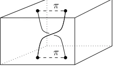
Definition 3.3. Each pathπin X◦ _{with endpoints}_v

1,v2inV determines a braid σπ in Γ(X,V) as follows (see [FN, §7]). We thicken the pathπ along its length (avoiding the other vertices), closing it off at the end points to form a (topological) disk. We give the boundary of the disk the clockwise orientation. The verticesv1andv2divide the boundary of the disk into two paths, one fromv1tov2

and the other from v2tov1. We defineγv1 to be the former andγv2 to be the latter. See Figure 3.

For v ∈ V such that v 6= v1,v2, we define γv(t) to be v for all t ∈ [0, 1]. Thenσπ is the braid (γv)v∈V. Note thatσπ only depends on the isotopy class of the image ofπin (X,V). In particular, it is unchanged ifπis reversed.

An example of a braidσπ is displayed as a picture (in the same way as in [All]) in Figure 4. In this figure only, we displayπas a dashed line to distinguish it from the braidσπ.

3.2 Interpretation of the generators

LetT be a triangulation of (S,M). LetQT be the quiver ofT. ThenQT has verticesI corresponding to the arcs inT. We denote the arc inT associated toi∈I byαi. The corresponding edge inGT is denoted πi. Letσi =σπi ∈Γ(X,VT) be the corresponding braid. We defineHT to be the subgroup

of Γ(X,VT0) generated by the braidsσi fori∈I.

Let T0 be an initial triangulation of (S,M) defined as follows. In the type An case, we choose a

[image:14.612.249.366.196.267.2]

(15)

⊲ ⊳

P α1

α2 α3

α4

α5

1 2 3 4 5

P

Q α1

α2

α3

α4

α5

α6 α7

1 2 3 4 5

6

[image:15.612.133.478.88.324.2]

7

Figure 5: Initial triangulations and the corresponding braid graphs and quivers

and Q (not homotopic to a boundary arc). We then take (noncrossing) arcs betweenP and every other marked point in M on the boundary of S not incident with a boundary arc incident with P. See Figure 5. Then the quiver QT0 associated toQT0 is a Dynkin quiver of type ∆. By Remark 2.3,

BQT₀ is isomorphic to the Artin braid group of type ∆.

Proposition 3.4. LetT0 be the triangulation of(X,M)defined as above. Then there is an

isomor-phism from HT0 to BQT₀ taking the braid σi to the generator si of BQT₀. Furthermore, in type An,

HT0 coincides withΓ(X,VT0), while in type Dn, HT0 is a subgroup of Γ(X,VT0)of index two.

Proof: For type An, see [FN] and the explanation in [All,§4]. For typeDn, note that the elements σi for i ∈I coincide with the generators hi defined in [All, §1] (via an isomorphism of the kind in Remark 3.2). The result then follows from [All, Thm. 1]. 2

The following lemma appears in [Ser, Th´eor`eme, part (iv)].

Lemma 3.5. Let A,B,C be three distinct points in X◦ _{and suppose there is a topological disk in}

X◦_{, with A, B and C lying in order clockwise around its boundary. Let AB denote the arc on this} boundary between A and B. We define BC and CA similarly. Then σABσBC =σBCσCA.

Theorem 3.6. LetT be an arbitrary tagged triangulation of(X,M). Then there is an isomorphism

from HT to BQT taking the braid σi to the generator si of BQT. Furthermore, in type An, HT

coincides withΓ(X,V), while in type Dn, HT is a subgroup ofΓ(X,V)of index two.

Proof: The result holds forT =T0by Proposition 3.4. Note that any triangulation can be obtained

from T0 by applying a finite number of flips of tagged triangulations. We show that the theorem is

true for an arbitrary tagged triangulationT by induction on the number of flips required to obtainT fromT0. To do this, it is enough to show that if the theorem holds for a tagged triangulationT and

(16)

[image:16.612.110.504.102.304.2]

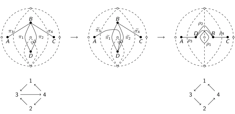
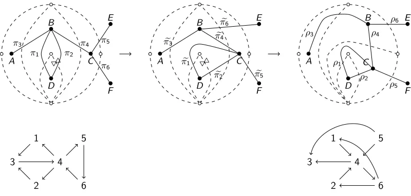
• C • D • F •E •_A • B π1 π3 π2 π5 π4 1 5 3 4 2 • C • D • F •E •_A • B e π1 e π3 e π2 e π5 e π4 • C • D • F •E •A • B ρ1 ρ3 ρ2 ρ5 ρ4 1 5 3 4 2

Figure 6: Flip involving an arc (α1) where two puzzle pieces of type I are glued

So we assume the result holds for a tagged triangulation T. Thus there is an isomorphism ψT : HT →BQT sendingσi tosi. We denote the corresponding elements ofHT′ byτi andti. The tagged

arcs inT are denoted byαi, fori∈I, and we denote the corresponding tagged arcs inT′ _by_βi_{, for} i ∈I. The edges ofGT are denoteπi, and we denote the edges ofGT′ byρi.

We define:

e

τi=

(

σ−1

k σiσk, if i→k in Q; σi, otherwise.

Then it is easy to see that HT is generated by theτie fori∈I.

We consider the possible types of flip that can occur, which are determined by the fact that T can be constructed out of puzzle pieces. Suppose first that T′ _{is the flip of} _T _{at an arc}_α _{where two} puzzle pieces of type (I) are glued together. We label the corresponding vertices in I by 1, 2, 3, 4, 5, for simplicity, and suppose we are flipping at the edge inT dual toα1. The braid graph local to the

flip is shown in the left hand diagram in Figure 6. Applying Lemma 3.5, we see that the middle figure shows paths πi_e with the property thatτi_e =σπei fori= 1, 2, 3, 4, 5.

Rotating vertices A and B clockwise, to get the right hand diagram in Figure 6, we obtain, via Remark 3.2, an isomorphism from HT to HT′ taking τie to τi for all i ∈ I. The inverse is an

isomorphism fromHT′toH_T takingτi toσ−1

k σiσkif there is an arrowi →kinQand toσiotherwise. Composing with the isomorphismϕk◦ψT, whereϕk is the isomorphism in Proposition 2.9, we obtain an isomorphism fromHT′ toBQ

T ′ takingτi toti as required. This proves the required result in type

A, so we are left with the type D case, where puzzle pieces of type II may occur.

We next consider a flip inside a puzzle piece of type II. We can apply essentially the same argument: see Figures 7 and 8. Here we draw the puzzle piece together with the two adjacent triangles, necessarily of type I (since there is only one cone point). We use the fact that in the right hand diagram of Figure 8, the resulting pathπ_e1 is isotopic to the pathρ1 in GT′, using the fact that the cone point

(17)

⊲⊳ ⊲⊳ ⊲ ⊳

⊲⊳ •

A

•

B

•

C

•

D

π3 π4

π1 π2

1

3 4

2

•

A

•

B

•

C

•

D

e

π3

e

π4

e

π1 πe2 •

A •

B

•

C

•

D

ρ3

ρ4

ρ1

ρ2

1

3 4

[image:17.612.114.501.143.322.2]

2

Figure 7: Flip (atα1) inside a puzzle piece of type II, first case

⊲⊳ ⊲⊳

•

A

•

B

•

C

•

D

π3 π4

π1 π2

1

3 4

2

•

A

•

B

•

C

•

D

e

π3 π_e4

e

π1 πe2 •

A •

B

•

C

•

D

ρ3

ρ4

ρ2

ρ1

1

3 4

2

[image:17.612.110.501.445.635.2]

(18)

⊲⊳ ⊲⊳ • A • B • C • D • E • F

π3 π4

π1 π2

π5 π6 1 3 4 2 5 6 • A • B • C • D • E • F e π3 e π4 e π4 e

π1 πe2

e π5 e π6 • A •

B C•

• D • E • F ρ5 ρ6

ρ3 ρ4

[image:18.612.108.513.99.291.2]

ρ2 ρ1 1 3 4 2 5 6

Figure 9: Flip involving an arc (α3) where puzzle pieces of type I and II are glued, first case

Note that the adjoining type I puzzle pieces (in Figures 7 and 8) may not occur, but the argument is easily modified to cover these cases. We also need to consider the flips from the right hand diagram in each case to the corresponding left hand one. We omit the details: a similar argument can be applied in these cases.

Finally, we need to consider a flip involving an arc where a puzzle piece of type I and a puzzle piece of type II have been glued together. These cases are shown in Figures 9 and 10: Figure 9 illustrates the case where the puzzle piece of type I is on the left of the puzzle piece of type II (when it is drawn as shown), while Figure 10 illustrates the case where it is on the right. Again, a similar argument applies in the case of flips from the right hand diagram to the left hand one in these cases. 2

4 Actions on categories

4.1 Quivers with potential

Fix an algebraically closed field F. To any quiver Q we can associate the path algebraFQ, which, as an F-vector space, has basis given by all paths inQ of length≥0, and the multiplication of two pathsp1 andp2 is their concatenationp1p2if p1ends andp2starts at the same vertex, and is zero

otherwise.

Let FQ≥n be the ideal of FQ generated by the paths in Q of length at least n. We can take the completionFQc ofFQ with respect toFQ≥1, which is defined as follows:

c

FQ= lim_←₋ n

FQ FQ≥n

={(an+FQ≥n)∞n=1|an∈FQ,ϕn(an+FQ≥n) =an−1+FQ≥n−1}

where the limit is taken along the chain of epimorphisms

FQ FQ≥1

և

ϕ2

FQ FQ≥2

և

ϕ3

FQ FQ≥3

(19)

⊲⊳ ⊲⊳ • A • B • C • D • E • F

π3 π4

π1 π2

π5 π6 1 3 4 2 5 6 • A • B • C • D • E • F e

π3 πe4

[image:19.612.104.504.99.290.2]

e π6 e π5 e π1 e π2 • B • C • A • D • E • F ρ6 ρ5 ρ4 ρ3 ρ1 ρ2 1 3 4 2 5 6

Figure 10: Flip involving an arc (α4) where puzzle pieces of type I and II are glued, second case

LetFQccyc denote the subspace of (possibly infinite) linear combinations of cycles inQ. Recall that a

potential for a quiverQis an element W ofFQccyc, regarded up to cyclic equivalence (and for which

no two cyclically equivalent paths inQ occur in the decomposition ofW). The pair (Q,W) is called a quiver with potential [DWZ], which we occasionally abbreviate to QP. The following definition is [DWZ, Definition 4.2].

Definition 4.1 (Derksen-Weyman-Zelevinsky). Let Q1andQ2be two quivers with the same vertex

setI and (Q1,W1) and (Q2,W2) be two QPs. A right equivalence between (Q1,W1) and (Q2,W2)

is an algebra isomorphism ϕ:FQd1→FQd2 such thatϕ(W1) is cyclically equivalent toW2 andϕis

the identity when restricted to the semisimple subalgebraFI ofFQd1.

A quiver with potential (Q,W) with W containing paths of length two or more istrivial if Q is a disjoint union of 2-cycles and there is an algebra automorphism of kQc preserving the span of the arrows of Q (a change of arrows) which takes W to the sum of the 2-cycles in Q. A quiver with potential (Q,W) is said to be reduced if W is a linear combination of cycles in Q of length 3 or more.

Thesplitting theorem [DWZ, Thm. 4.6] states that every quiver with potential can be written as a direct sum of a reduced quiver with potential and a trivial quiver with potential which are unique up to right equivalence.

Let (Q,W) be a quiver with potential, and letk be a vertex ofQ not involved in any 2-cycles. By replacing W with a cyclically equivalent potential on Q if necessary, we can assume that none of the cycles in the decomposition of W start or end atk. We denote byµkf(Q,W) the non-reduced mutation of (Q,W) atkinQ, as defined in [DWZ,§5]. Then the right equivalence class offµk(Q,W) is determined by the right equivalence class of (Q,W) by [DWZ, Thm. 5.2]. Themutationµk(Q,W) of (Q,W) atk is then defined to be the reduced component of_fµk(Q,W), and is uniquely determined up to right equivalence, given the right equivalence class of (Q,W).

(20)

potential (Q′_,_W′_{) is}_{mutation-Dynkin} _{if it can be obtained by repeatedly mutating a Dynkin quiver} with potential in the above sense. For the rest of Section 4.1we will restrict to Dynkin types A and D.

Let (S,M) be the Riemann surface with marked points associated to ∆ as in Section 3. So, if ∆ =An, we takeS to be a disk withn−3 points on its boundary, and if ∆ =Dn, we takeS to be a disk with one marked point in its interior and nmarked points on its boundary.

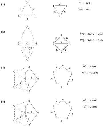
LetQbe a mutation-Dynkin quiver. By [FoSTh],Q=QT for some tagged triangulationT of (S,M). Let W,W′ _{be the sum of the terms coming from local configurations in} _T _{as shown in Figure 11} (where in (c) and (d) there are at least three arcs incident with the interior marked point).

ThenWT is the potential given by taking the sum of the induced cycles inQT (i.e. induced subgraphs ofQT which are cycles), andWT′ is the potential associated toT in [LF12,§3], taking the parameter associated to the internal marked point (if there is one) to be equal to −1. Then we have the following:

Lemma 4.2. The potentials WT and WT′ are right equivalent.

Proof: We assume we are in caseDn, since the two potentials coincide in caseAn. If the interior marked point is as in case (c) of Figure 11 (with at least 3 arcs incident with it), then there is a unique triangle in T with sides 1 and 2. We label the arrows in the corresponding 3-cycle inWT or W′

T by a,x,y, in order around the cycle. Then the automorphism ϕofkQdT negatinga andx and taking each other arrow to itself gives a right equivalence between WT andWT′, sincea andx are not involved in any other terms in any of these potentials.

If the interior marked point is as in case (d), then WT andWT′ coincide. 2

We recall the following special case of [LF12, Thm. 8.1].

Theorem 4.3. [LF12] LetT,T′ _{be triangulations of}₍_S_,_M₎_{. If}_T′ _{is obtained from}_T _{by flipping at}

an arc αk then µk(QT,WT′)is right equivalent to(QT′,W_T′′).

By [DWZ, Thm. 7.1], it follows from this that the quiver of µk(QT,WT) coincides with the quiver obtained from QT by Fomin-Zelevinsky quiver mutation at k.

Hence we can effectively ignore potentials:

Proposition 4.4. Any mutation-Dynkin quiver with potential(Qe,fW)of type A or D is right

equiv-alent to (Qe,WQe), where WQe is the sum of all chordless cycles inQ.e

Proof: Note that a Dynkin quiver with zero potential is of the form (QT,WT) for some triangulation T (see [FoSTh]). Suppose that (Qe,fW) is obtained from a Dynkin quiver with zero potential by iterated mutation in the sense of [DWZ]. Then, by Theorem 4.3 and Lemma 4.2, (Qe,Wf) is right equivalent to (QT,WT) for some triangulation T of (S,M). 2

Note that an alternative proof of Proposition 4.4 would be to compute the mutation of a quiver with potential (QT,WT′) directly, and show that it is right equivalent to (QT′,W′

T′). This is not too

(21)

⊲⊳

3 2 1

5 ₄

3 2 1

5 ₄

⊲⊳

⊲ ⊳

⊲⊳

⊲⊳ ⊲⊳ (a)

1 2

3

1 2

3 a

b c

WT : abc

W′ T : abc

(b)

1 2

3 4 3 4

1

2 a2 a1

b2 b1

c

WT : a1a2c+b1b2c

W′

T : a1a2c+b1b2c

(c)

3 2

1

5 ₄

b a

e

d

c

WT : abcde

W′

T : −abcde

(d)

3 2

1

5 ₄

b a

e

d

c

WT : abcde

W′

[image:21.612.121.481.164.608.2]

T : abcde

(22)

4.2 Differential graded algebras and modules

Let F be an algebraically closed field. We think ofF as a gradedF-algebra concentrated in degree 0. If V =LVi is a graded F-module then let V[j] be the graded F-module with (V[j])i =Vi+j. If f : V → W is a map of graded vector spaces with homogeneous components fi : Vi → Wi then let f[j] : V[j] → W[j] be the map of graded vector spaces with homogeneous components f[j]i : V[j]i → W[j]i defined by f[j]i(v) = (−1)jfi+j(v) for v ∈ V[j]i = Vi+j. Thus [1] is an endofunctor of the category of gradedF-modules, called the shift functor.

We say that a map f : V → W of graded vector spaces has degree i to mean that f is a map V →W[i]. We use the Koszul sign rule for gradedF-algebras, so if f :V →V′ _and_g _:_W _→_W′ are maps of gradedF-modules of degree mandnthen

(f ⊗g)(v⊗w) = (−1)in_f₍_v₎_⊗_g₍_w₎

forv ∈Vi andw ∈W.

A unital differential graded algebra (or dg-algebra, or dga) overFis a gradedF-algebraA=L_i∈ZAi with multiplication m : A⊗FA → A of degree 0 together with a unit ι : F ֒→ A and an F-linear differentiald:A→Aof degree +1. These should satisfy the following relations:

• the associativity relationm◦(1⊗m) =m◦(m⊗1);

• the boundary relationd2_{= 0;}

• the Leibniz relationd◦m=m◦(1⊗d+d⊗1);

• the unital relationm◦(idA⊗ι) =m◦(ι⊗idA), which should agree with theF-algebra structure ofA.

We often denote our dga by (A,d), or simply byA. Each dga (A,d) has an underlying unital graded algebra, obtained by simply forgetting the differential, which we denote u(A).

A left module M forA is a graded left F-module M with a left action mM :A⊗M →M of u(A) together with a mapdM:M →M of degree +1, called adifferential, such that

dM◦mM=mM◦(1⊗dM+d⊗1).

We always have the regular module M =Awith dM =d andmM =m. Similarly, a right module M for A is a graded right F-module M with a right action mM : M ⊗A → M of u(A) together with a differential dM such that dM◦mM = mM◦(1⊗d+dM ⊗1). If (M,dM) is an A-module, then (M[1],dM[1]) is also anA-module, which we sometimes just write asM[1]. Modules forAare modules foru(A), simply by forgetting the differential.

A map f :M→N of leftA-modules is a degree 0 map ofu(A)-modules such thatf commutes with the differentials: dN◦f =f◦dM. We thus obtain a categoryA-Mod of leftA-modules, and we write the morphism spaces in this category as HomA-Mod(M,N). A-Mod is anF-category: each morphism

space is anF-module.

Given two differential algebras (A,dA) and (B,dB), anA-B-bimodule (M,dM) is a gradedF-module which is a left (A,dA)-module with left action mℓ _{and a right (}_B_,_dB_{)-module with right action} _mr where the two actions commute: mr_◦₍_mℓ_⊗_id

(23)

andA-B-bimodules with leftA⊗FBop-modules, whereBop denotes the algebraB with the order of multiplication reversed. A map of bimodules should commute with the differential on both the left and the right, and we obtain anF-category A-Mod-B ofA-B-bimodules.

Given a map f :M →N of left A-modules, we can construct a new left A-module called thecone of f, denoted cone(f). As a left module foru(A), we have cone(f) =N⊕M[1]. The differential is

given by:

dN 0 f[1] dM[1]

.

IfLis isomorphic to cone(f) for some mapf :M →N, we say thatLis anextensionofM byL[−1].

We will use the following lemma, whose proof follows immediately from the definitions, repeatedly.

Lemma 4.5. Let f :M →N be a map in A-Mod.

(i) Let F :A-Mod→B-Modbe an additive functor which commutes with the shift functor. Then we have an isomorphismcone(Ff)∼=Fcone(f)in B-Mod.

(ii) For any commutative diagram

M f //

ϕM

∼

N

ϕN

∼

M′ f′ _//_N′

in A-Mod where bothϕM andϕN are isomorphisms, we have an isomorphism ϕN⊕ϕM[1] : cone(f)→cone(f′₎_{of A-modules.}

Let (A,dA), (B,dB), and (C,dC) be dgas. If (M,dM) is an A-B-bimodule and (N,dN) is an A-C -bimodule then let Homi_A(M,N) be the space of all graded left u(A)-module mapsf : M → N of degree i. Note that we do not require that these maps commute with the differential. We define HomA(M,N) = Li∈_ZHom

i

A(M,N), and this is a graded u(B)-u(C)-bimodule. We also have a version for right modules, which we write as HomAop(M,N).

Note the distinction between HomA(M,N) and the hom spaces in the category A-Mod. With the differentiald(f) =dN◦f−(−1)i_f_◦_dM_for_f _∈_Homi

A(M,N), HomA(M,N) becomes aB-C-bimodule. Similarly, if (M,dM) is an B-A-bimodule and (N,dN) is aC-A-bimodule, HomAop(M,N) is aC-B

-bimodule. HomA(−,−) is the internal hom in the bimodule category, and we can recover the hom spaces inA-Mod as the 0-cycles of HomA(M,N).

If (M,dM) is an A-B-bimodule and (N,dN) is aB-C-bimodule then let M⊗B N denote the space M⊗u(B)N. It is a gradedu(A)-u(C)-bimodule: ifm∈Mi andn∈Nj thenm⊗nhas degreei+j.

With the differential dM⊗idN+ idM⊗dN, it becomes anA-C-bimodule.

For anA-B-bimodule (M,dM), we thus have functorsM⊗B−:B-Mod→A-Mod and HomA(M,−) : A-Mod→B-Mod. The functorM⊗B−is left adjoint to HomA(M,−). For (N,dN) a leftA-module, the counit evN : M ⊗B HomA(M,N)→ N of the adjunction is the evaluation map, which acts as x⊗f 7→(−1)ij_f₍_m_{) for}_x _∈_Mi _and_f _∈_Homj

A(M,N).

4.3 Derived categories

(24)

If A is a graded vector space and d is a differential, i.e., a degree +1 endomorphism of A which satisfies d2 _{= 0, then the} _i_{th homology of} _A_{, denoted} _Hi₍_A_{), is the subquotient ker}_di/_im_di

−1,

where di : Ai → Ai+1 denotes the restriction of d to Ai. If (A,d) is a dga then the homology

H(A) =LHi(A) is a graded algebra, and ifM is a leftA-module thenH(M) =LHi(M) is a left H(A)-module. In fact, taking homology is a functor from the category ofA-modules to the category of graded H(A)-modules. We say that a leftA-module M is acyclic if H(M) = 0, and that a map f :M→N ofA-modules is aquasi-isomorphism ifH(f) is an isomorphism.

Thecategory up to homotopy ofA-Mod, denoted K(A), is theF-category whose objects are all left A-modules and whose morphism spaces, forM,N∈A-Mod, are HomK(A)(M,N) =H0HomA(M,N). Thederived category of A, denoted D(A), is theF-category obtained by localizing K(A) at the full subcategory of acyclic A-modules. As a map of modules is a quasi-isomorphism if and only if its cone is acyclic, this is equivalent to localizing K(A) at the class of all quasi-isomorphisms. So we have a canonical functor K(A)→D(A), which we call the projection functor. The finite-dimensional derived category, denoted Dfd(A), is the full subcategory of D(A) on objects with finite-dimensional

total homology, i.e., onA-modulesM such that H(M) is a finite-dimensionalF-vector space.

Let (A,dA) be a dga. We say that:

• P ∈ A-Mod is indecomposable projective if it is an indecomposable direct summand of the regular module,

• P ∈A-Mod isrelatively projective if it is a direct sum of shifts of indecomposable projective modules, and

• P ∈ A-Mod is cofibrant if, for each surjective quasi-isomorphism f : M → N, the map HomA-Mod(P,f) : HomA-Mod(P,M)→HomA-Mod(P,N) is surjective.

The following result (see [Kel94, Section 3] and [KY, Proposition 2.13]) characterizes cofibrant mod-ules.

Proposition 4.6 (Keller). An A-module P is cofibrant if and only if it is an iterated extension of a

relatively projective module by other relatively projective modules, possibly infinitely many times.

Let A-cofib denote the full subcategory of K(A) on the cofibrant objects. The projection functor K(A)→D(A) induces an equivalence A-cofib→∼ D(A). Each A-module M has a cofibrant replace-ment, defined up to quasi-isomorphism and denotedpM, which can be realized as the image of M under the left adjoint D(A)→K(A) to the canonical projection functor [Kel06, Proposition 3.1].

Let (B,dB) be another dga and letF :A-Mod→B-Mod be an additive functor. ThenF preserves chain homotopies, so induces a functor K(F) : K(A)→K(B). If K(F) preserves quasi-isomorphisms then, by the universal property of localization, it induces a functor D(F) : D(A)→ D(B). If P ∈ A-Mod-B is cofibrant as a left A-module then, by [Kel94, Theorem 3.1(a)] and [KY, Proposition 2.13], HomA(P,−) preserves acyclic modules, and so preserves quasi-isomorphisms. By imitating the proof of [Kel94, Theorem 3.1(a)] we see that if P ∈ A-Mod-B is cofibrant as a right B-module then P⊗B− also preserves acyclic modules. We often write P⊗B −and HomA(P,−), instead of D(P⊗B−) and D(HomA(P,−)), for the induced functors D(B)→D(A) and D(A)→D(B).

For an arbitrary M ∈A-Mod-B, we can obtain a functor M⊗L

B −: D(B)→D(A), known as the left derived functor ofM⊗B−, by composing the cofibrant replacement functor D(B)→K(B), the tensor functor K(M⊗B −) : K(B)→K(A), and the projection functor K(A)→D(B). By [Kel94, Lemma 6.3(a)], we have an isomorphism M ⊗L

(25)

Lemma 4.7. Let M ∈Mod-B.

(i) We have a natural isomorphism of functorspM⊗B− ∼=M⊗L B−.

(ii) If M is cofibrant then we have a natural isomorphism of functors M⊗B− ∼=M⊗L B−.

Proof:

(i) We need to show that for eachN ∈B-Mod there is a quasi-isomorphismϕN : pM⊗B N → M⊗BpN such that, for all mapsf :N→N′_{, the diagram}

pM⊗BN ϕN //

pM⊗f

M⊗BpN

M⊗pf

pM⊗BN′ ϕN′

//M⊗BpN′

commutes. Consider the following diagram:

pM⊗BpN

pM⊗πN

πM⊗pN

pM⊗BpN′

pM⊗πN′

πM⊗pN ′

pM⊗BN_ _ _ _ϕN_ _ _ _//

pM⊗f

,, Y Y Y Y Y Y Y Y Y Y Y Y Y Y Y Y Y Y Y Y Y Y Y Y Y Y Y Y Y Y

Y M⊗BpN

M⊗pf

,, Y Y Y Y Y Y Y Y Y Y Y Y Y Y Y Y Y Y Y Y Y Y Y Y Y Y Y Y Y Y Y Y

pM⊗BN′ ϕN′

// _ _ _ _ _ _ _

_ M⊗BpN′

As pM and pN are cofibrant and πM and πN are quasi-isomorphisms, both pM ⊗πN and πM⊗pN are quasi-isomorphisms, so we can defineϕN = (πM⊗pN)◦(pM⊗πN)−1 _{and it}

is a quasi-isomorphism. Then to check naturality we need to show that

(M⊗pf)◦(πM⊗pN)◦(pM⊗πN)−1_{= (}_πM_⊗

pN′₎_◦₍

pM⊗πN′)−1◦(pM⊗f).

By the bifunctoriality of the tensor product, the left hand side is equal to

(πM⊗pN′)◦(pM⊗pf)◦(pM⊗πN)−1

so we just need to show that

pf ◦π_N−1=π_N−′1◦f

but this follows from the functorialityf ◦πN =πN′◦pf of the cofibrant replacement functor p.

(ii) We just need to show that, forMcofibrant, there is a natural isomorphismM⊗B− ∼=pM⊗B−, and then the result will follow by part (i) of the lemma. This follows becauseπM :pM →M is a quasi-isomorphism and by the bifunctoriality of the tensor product.

(26)

If the functorM⊗L

B −is an equivalence D(B) ∼

→D(A), we say thatM is a tilting module.

We say that a module M is of finite projective dimensionif its cofibrant replacement is an iterated extension of finitely many shifted indecomposable projective modules.

The following basic lemma will also be useful. It can be found as [Kel94, Lemma 6.2(a)]. We include a proof for the convenience of the reader.

Lemma 4.8. Let M be a left A-module of finite projective dimension and let P be its cofibrant

replacement. Then we have a natural isomorphism of functors

HomA(P,A)⊗A− ∼

→HomA(P,−) :A-Mod→F-Mod .

Proof: First note that, for anyP∈A-Mod, we always have a natural transformation

HomA(P,A)⊗A− →HomA(P,−)

obtained by staring with the map

ev⊗1 : (P⊗FHomA(P,A))⊗AM→A⊗AM,

using the associativity isomorphism to obtain a map

P⊗F(HomA(P,A)⊗AM)→A⊗AM,

using the adjunction

HomF(HomA(P,A)⊗AM, HomA(P,A⊗AM))∼= HomA(P⊗F(HomA(P,A)⊗AM) ,A⊗AM),

and finally using the natural isomorphismA⊗AM ∼=M.

To show that our natural transformation is an isomorphism, we use induction on the number of times we need to extend a summand of the regular module to obtainP. We handle the base case as follows: the natural transformation is certainly an isomorphism whenP is the regular module and so, as hom functors commute with finite direct sums, it is an isomorphism for all summands of the regular module. For our inductive step, suppose the lemma holds for P1 andP2, and letP= cone(f) for some map

f :P1→P2. Then, forM ∈A-Mod, one can check that the map HomA(P,A)⊗AM→HomA(P,M) comes from the commutative diagram

HomA(P1,A)⊗AM

HomA(P2,A)⊗AM Hom(f,A)⊗M

oo

HomA(P1,M) HomA(P2,M) Hom(f,M)

oo

as in the construction from the second half of Lemma 4.5, where the vertical maps come from the natural transformation described above. Therefore, as both vertical maps are isomorphisms by induction, HomA(P,A)⊗AM→HomA(P,M) is an isomorphism. 2

4.4 Spherical twists

Our references are [ST, RZ, Gra1].

(27)

• M is ad-Calabi-Yau object, i.e., we have an isomorphism

HomDfd(A)(M,N)= Hom∼ Dfd(A)(N,M[d])

∗

which is functorial inN, and

• L_i∈ZHomDfd(A)(M,M[i]) is isomorphic as a graded algebra toF[x]/hx

2_i_{, with}_x _{in degree}_d_.

Associated to any spherical objectM, we have a spherical twist functorFM: Dfd(A)→Dfd(A) which

is defined as follows. First, let P=pM be a cofibrant replacement ofM. Then letXM be the cone of the following map ofA-A-bimodules:

P⊗_FHomA(P,A)

ev

→A

where the nonzero map is the obvious evaluation map. As both HomA(P,A) andAare cofibrant,XM is cofibrant as a right A-module. Then we define the spherical twist atM by

FM =XM⊗A−: Dfd(A)→Dfd(A).

The spherical twist is an autoequivalence of Dfd(A) (soXM is a tilting module).

Note that, by Lemmas 4.5 and 4.8, if M has finite projective dimension then

FM(N)∼=P⊗FHomA(P,N)

ev

→N.

We will need a simple result on the commutation relation of spherical twists with derived equivalences. It is a generalization of [ST, Lemma 2.11].

Proposition 4.9. Let A,B be dgas. Let T ∈ B-Mod-A be a tilting module and Φ = T ⊗L

A−: Dfd(A)→ Dfd(B)be the associated derived equivalence. Let M ∈A-Modhave finite dimensional

total homology and suppose it is d-spherical, for some d ∈ Z. Suppose thatΦ(M)∈ B-Mod has finite dimensional total homology. Then Φ(M) is also d-spherical and we have an isomorphism of functors

Φ◦FM∼=FΦ(M)◦Φ : Dfd(A)

∼

→Dfd(B).

In particular, we have an isomorphism

FΦ(M)∼= Φ◦FM◦Φ−1: Dfd(B)

∼

→Dfd(B)

where Φ−1_{is the quasi-inverse functor of} _Φ_.

Proof: As Φ : Dfd(A)→Dfd(B) is a derived equivalence it has quasi-inverse Φ−1: Dfd(B)→Dfd(A),

and so we have isomorphisms

HomDfd(B)(Φ(M), Φ(M)[i])∼= HomDfd(A)(M,M[i])

and

HomDfd(B)(Φ(M),N)∼= HomDfd(A)(M, Φ

−1₍_N₎₎

∼

= HomDfd(A)(Φ

−1₍_N_),_M_[_d_])∗

∼

= HomDfd(B)(N, Φ(M)[d])

∗ ,

the second natural in N ∈ Dfd(B), using the facts that M is a d-Calabi-Yau object and the shift

(28)

By Lemma 4.7 we may assume that T is cofibrant as a rightB-module and that Φ =T ⊗A−. We want to show thatT ⊗AXM⊗A− ∼=XΦ(M)⊗B T⊗A−, so it is enough to check that we have an

isomorphism T⊗AXM ∼=XΦ(M)⊗BT in Dfd(B⊗FAop). To construct this isomorphism, we use the following extension of Lemma 4.5, which follows from the triangulated 5-lemma: for any commutative diagram

M f //

ϕM

∼

N

ϕN

∼

M′ f′ _//_N′

in B-Mod-AwithϕM andϕN both quasi-isomorphisms, we have a quasi-isomorphismϕN⊕ϕM[1]:

cone(f)→cone(f′_).

As above, write P =pM. Then, by the first part of Lemma 4.5, we just need to find two vertical maps which are quasi-isomorphisms and make the following diagram commute:

T⊗AP⊗FHomB(T ⊗AP,B)⊗B T

ev⊗1T

//

∼

B⊗BT

∼

T⊗AP⊗FHomA(P,A)

1T⊗ev

//T ⊗AA

Our plan is to do this in stages: we will show that the vertical maps in the following diagram exist, and are quasi-isomorphisms, and that the diagram commutes:

T⊗AP⊗_FHomB(T ⊗AP,B)⊗B T

ev⊗1T

//

∼

B⊗BT

=

T⊗AP⊗_FHomB(T ⊗AP,B⊗B T)

ev

//

∼

B⊗BT

∼

T⊗AP⊗FHomB(T ⊗AP,T ⊗AA)

ev

//

∼

T ⊗AA

=

T⊗AP⊗FHomA(P,A)

1T⊗ev

//T ⊗AA

Let us show that the first square commutes. We’ll introduce some temporary notation for the rest of this proof. LetF andG denote the functorsF =T ⊗AP⊗F−andG = HomB(T ⊗AP,−), so F is left adjoint toG, and letH denote the functor− ⊗B T. Then we have unit and counit natural transformationsε:FG →1 andη: 1→GF, and a natural isomorphism ζ:HF →∼ FH coming from the associativity isomorphism for tensor products. We first need to define a map

HFGB=T ⊗AP⊗F HomB(T ⊗AP,B)⊗B T →T ⊗AP⊗F HomB(T⊗AP,B⊗BT) =FGHB

We define this as the composite

HFGBζ→GBFHGB FηHGB

→ FGFHGB FGζ

−1_GB

→ FGHFGBFGHεB

→ FGHB.

(29)

diagram commutes, we break it up into smaller diagrams as follows:

HFGB

∼ ζGB

HεB

//HB

FHGB 1 //

FηHGB

FHGB ∼

ζ−1GBJJJJ_%% J J J J J FGFHGB ∼ FGζ−1GB

εFHGB 88 r r r r r r r r r r HFGB HεB

CC

FGHFGB FGHεB

// εHFGB 44 i i i i i i i i i i i i i i i i i FGHB εHB OO

Now we see that both squares commute by the naturality ofε, the triangle commutes by the triangle identity εF ◦Fη = 1F, and the pentagon commutes because the isomorphisms are defined byζ and its inverse.

To define the second square we use the obvious composite isomorphism B⊗BT →∼ T →∼ T ⊗AA. This commutes because the evaluation map is a counit, and therefore a natural transformation.

To show that the third square commutes, we introduce some more notation. Let F′ _and_G′ _denote the functorsF′ ₌_P_⊗

F−andG′ = HomA(P,−), soF′is left adjoint toG′, and letH′andI′ denote the functorsH′ ₌_T_⊗A₋_and_I′ _{= Hom}

B(T,−), soH′ is left adjoint (in fact, quasi-inverse) toI′. We denote the counit and unit maps of the first adjunction byε′_:_F′_G′_→_{1 and}_η′_{: 1}_→_G′_F′_{, and} of the second adjunction by ε′′ _: _H′_I′ _→_{1 and} _η′′ _{: 1} _→ _I′_H′_{. Note that, because} _H′ _{induces an} equivalence of derived categories,ε′′ _and_η′′ _{give quasi-isomorphisms when applied to any object.}

Using the associativity isomorphism for tensor products we have a natural isomorphism of functors F ∼=H′_F′_{, and by the uniqueness of right adjoints (or by using the tensor-hom adjunctions directly)} this gives us another natural isomorphismG ∼=G′_I′_.

We now redraw our final square, breaking it up into smaller diagrams:

FGH′_A ε

′ H′_A

//

∼

H′_A

H′_F′_G′_I′_H′_A H

′

ε′_I′_H′_A

//H′_I′_H′_A

ε′′H′A

:: t t t t t t t t t

H′_F′_G′_A H

′

ε′A

// H′ F′ G′ η′′ A OO

H′_A H′ η′′ A dd JJJ JJJ JJJ 1 OO

Here, the top square commutes by definition of the isomorphisms F ∼= H′_F′ _and _G ∼₌ _G′_I′_{, the} triangle commutes by the triangle identityε′′_H′_◦_H′_η′′_{= 1}

H′, and the bottom square commutes by

the naturality ofε′_.

2

We now describe the braid relations for spherical twists, as in Propositions 2.12 and 2.13 of [ST] (see also [RZ, Gra2]).

Proposition 4.10. Suppose that M and N are spherical objects ofDfd(A)and let

(M,N) = dim_FM n∈Z

HomDfd(A)(M,N[n]).

Let FM,FN : Dfd(A)

∼

(30)

• If(M,N) = 0then FM◦FN ∼=FN◦FM;

• if(M,N) = 1 then FM◦FN◦FM∼=FN◦FM◦FN.

4.5 Ginzburg dg-algebras

There is a by now well-known method to associate a differential graded algebra to a quiver with potential ([Gin, Section 5], [KY, Section 2.6]).

Let (Q,W) be a quiver with potential. Construct a new quiverQ by adding arrows toQ: for each arrow a:i→j inQ we add a new arrowa∗_:_j _→_i_{, and for each vertex} _i _in_Q _{we add a new arrow} ti :i →i. We view Q as a graded quiver with the arrows ofQ in degree 0, the arrowsa∗ _{in degree} −1, and the arrowsti in degree−2. This induces a grading on the path algebraFQ ofQ such that the degree 0 part (FQ)0is just the path algebra ofFQ ofQ. LetJ denote the ideal ofFQ generated

by the arrows ofQ, and letFQc denote the completion of the graded algebraFQ with respect to J, as in Section 4.1.

We define a differential d on FQc by imposing thatd is zero on each idempotent ei associated to a vertex i of Q, specifying how d acts on arrows of Q, and then extending to the rest of FQc using the Leibniz rule and continuity. For degree reasons, we must have d(a) = 0 for each arrowa ofQ. For arrows a∗_{, we set} _d₍_a∗_{) =}_∂aW_{, where}_∂a _{denotes the cyclic derivative. For arrows} _ti_{, we set} d(ti) =ei(Paa∗₋_a∗_a₎_ei_{, where we sum over all arrows}_a _of _Q_{. Then Γ}

Q,W = (FQc,d) is called theGinzburg dgaof (Q,W).

Note that [KY, Lemma 2.9] if (Q1,W1) and (Q2,W2) are right equivalent, then we have an

isomor-phism of dgas ΓQ1,W1 ∼= ΓQ2,W2. Hence, if we are working with quivers with potential of mutation type

A or D, by Proposition 4.4 we only need to consider the Ginzburg dgas ΓQ,WQ, and so can denote

them ΓQ.

Keller and Yang showed [KY, Theorem 3.2] that QP-mutation lifts to equivalences of derived cat-egories of Ginzburg dgas. Suppose that (Q,W) is a QP and that (Q′_,_W′_{) =}_µk₍_Q_,_W_{) for some} k ∈I.

Theorem 4.11(Keller-Yang). There is a tilting complex T which gives an equivalence of triangulated