This is a repository copy of
A reduced basis model with parametric coupling for
fluid-structure interation problems
.
White Rose Research Online URL for this paper:
http://eprints.whiterose.ac.uk/81804/
Version: Submitted Version
Article:
Lassila, T., Quarteroni, A. and Rozza, G. (2012) A reduced basis model with parametric
coupling for fluid-structure interation problems. SIAM Journal on Scientific Computing , 34
(2). A1187 - A1213. ISSN 1064-8275
https://doi.org/10.1137/110819950
[email protected] https://eprints.whiterose.ac.uk/
Reuse
Unless indicated otherwise, fulltext items are protected by copyright with all rights reserved. The copyright exception in section 29 of the Copyright, Designs and Patents Act 1988 allows the making of a single copy solely for the purpose of non-commercial research or private study within the limits of fair dealing. The publisher or other rights-holder may allow further reproduction and re-use of this version - refer to the White Rose Research Online record for this item. Where records identify the publisher as the copyright holder, users can verify any specific terms of use on the publisher’s website.
Takedown
If you consider content in White Rose Research Online to be in breach of UK law, please notify us by
FOR FLUID-STRUCTURE INTERACTION PROBLEMS
TONI LASSILA† ‡, ALFIO QUARTERONI† §,AND GIANLUIGI ROZZA†
Abstract. We present a new model reduction technique for steady fluid-structure interaction problems. When the fluid domain deformation is suitably parametrized, the coupling conditions between the fluid and structure can be formulated in the low-dimensional space of geometric param-eters. Moreover, we apply the reduced basis method to reduce the cost of repeated fluid solutions necessary to achieve convergence of fluid-structure iterations. In this way a reduced order model with reliable a posteriori error bounds is obtained. The proposed method is validated with an exam-ple of steady Stokes flow in an axisymmetric channel, where the structure is described by a simexam-ple 1-d generalized string model. We demonstrate rapid convergence of the reduced solution of the parametrically coupled problem as the number of geometric parameters is increased.
AMS subject classifications. 65N30, 74F10, 76D07
Key words. fluid-structure interaction, model reduction, incompressible Stokes equations, re-duced basis method, free-form deformation
1. Introduction. The numerical simulation of Fluid-Structure Interaction (FSI) problems is an important topic in wide areas of engineering and medical research. Concerning the latter, of great importance is the modelling of blood flow in the large arteries of the human cardiovascular system, where pulsatile flows combined with a high degree of deformability of the arterial walls together cause large displacement effects that cannot be neglected when attempting to accurately model the flow dy-namics of the system. High fidelity computational fluid dydy-namics and structural mechanics solvers based on, for example, the Finite Element Method (FEM) need to be combined in a framework that is challenging both from a mathematical as well as implementation viewpoint. For an overview of cardiovascular modelling techniques we refer to [42, 44] and the book [14]. The complexity and nonlinearity of FSI problems has until recently limited the scope of physically meaningful simulations to just small and isolated sections of arteries. When attempting to consider the entire cardiovas-cular system as a complex network of different time and spatial scales, Model Order Reduction (MOR) techniques can accurately and reliably reduce the nonlinear FSI models to computationally more cost-efficient ones.
In the geometric multiscale approach to MOR [13] the flow network is decomposed to smaller parts that are joined together using physical coupling conditions, and each part of which is modelled at a level necessary to capture the relevant local dynamics of the system. The target for our proposed reduced model is those parts of the car-diovascular network, where a full fidelity 3-d Navier-Stokes solution is not necessary, but where fluid-structure interaction effects are still important. The reduced model should fulfill two conditions: (i) it should have certified a posteriori error bounds that can be tuned to the user’s requirements, and (ii) it should have sufficiently low online computational memory requirements to fit on one parallel node of a supercomputer.
†Modelling and Scientific Computing (CMCS), ´Ecole Polytechnique F´ed´erale de Lausanne,
Lau-sanne, Switzerland ([email protected], [email protected], [email protected]). Support provided by ERC-Mathcard Project (ERC-2008-AdG 227058).
‡Department of Mathematics and Systems Analysis, Aalto University, Helsinki, Finland.
Sup-ported by the Emil Aaltonen Foundation.
§Modelling and Scientific Computing (MOX), Politecnico di Milano, Milan, Italy.
An important aspect of any large-displacement FSI problem is finding the config-uration of the interface between fluid and structure. The process is typically iterative: a trial configuration of the geometry is used to solve the fluid and structure subprob-lems, the coupling conditions are tested, and if they are not satisfied within a desired degree of accuracy then the trial configuration is updated and the step is repeated. A traditional approach to FSI is that the discrete mesh is updated on each iteration by moving the boundary nodes and adjusting the interior mesh points to ensure mesh quality. This approach leads to a large number of coupling variables (the total number of mesh points on the free boundary). An external parametrization of the geometry can be used to drive down the number of coupling variables. When considering sim-ple flow geometries the shape of the deformable wall can be directly parametrized e.g. with splines. For realistic geometries it might be necessary to parametrize the geometry in a way that is relatively independent of its description.
There are many shape parametrization methods to choose from. Comparisons of different shape parametrization techniques from a fluid dynamics viewpoint can be found in [52], and from a model reduction viewpoint in [33]. We propose to describe the deformations of the fluid channel with Free-Form Deformations (FFDs) [53]. They are a technique for smooth parametric deformations of arbitrary shapes embedded in the grid of control points. FFDs can be used to give a flexible and global parametric deformation of a fixed reference domain that is completely independent of the shape and its computational mesh. Model reduction for FFD-based shape parametrizations has been previously considered for the shape design of airfoils in potential [27] and thermal flows [50]. In cardiovascular applications, FFDs have been used to track the motion of the left ventricle (see [34] for a review), and to solve an optimal shape design problem of an aorto-coronaric bypass anastomoses [32].
After parametrizing the geometry with a FFDs we need to address the coupling between fluid and structure. We use the deformation parameters of the FFD as coupling variables. A fixed point coupling algorithm can be written in the parameter space rather than the displacement space. Again an iterative procedure is needed to ensure the coupling conditions are satisfied to a desired tolerance. Thus a potentially large number of parametric PDE solutions for the fluid equations need to be performed in different parametric configurations.
To reduce the memory requirements and the online computational cost of solving the fluid system, we apply the Reduced Basis (RB) method (originally proposed and analyzed in [1, 11, 37, 41]). It is a reliable MOR method for parametric PDEs. An overview can be found in [49] and a more detailed exposition in [38]. The attractive-ness of these methods is based on their ability to give certified a posteriori bounds on the error of the field solutions and their outputs when compared to the underlying FEM solution. We use the reduced basis method to reduce the computational cost of the steady Stokes equations in different configurations of the geometry.
2. The steady fluid-structure interaction model. We use the following standard notations: Ω ⊂ Rd, d = 1,2,3, is a bounded open set, Hk(Ω) is the Sobolev space of functions with weak derivatives up to orderk square-integrable on
X, Hk−1/2(∂Ω) is the space of functions that are traces of Hk(Ω) on the boundary
∂Ω,Hk
0(Ω) is the subspace of functions whose trace vanishes on ∂Ω; Ck,α(Ω) is the space of functions with derivatives up to orderkbeing H¨older-continuous with expo-nent 0< α≤1 (if α= 1 these are the Lipschitz-continuous functions); L2(Ω) is the space of square-integrable functions, andL∞(Ω) is the space of essentially bounded functions on Ω.
Ωo Γw
Γin x2
x1 φ
η(x1)
R(x1)
[image:4.612.115.395.227.359.2]Γout
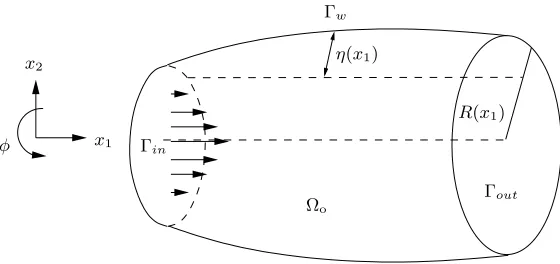
Fig. 2.1.Axisymmetric flow geometry for the fluid-structure interaction model problem
2.1. Fluid model: the steady incompressible Stokes equations. We as-sume the flow geometry represented in Fig. 2.1 that is axisymmetric with cylindrical coordinates (x, φ) = (x1, x2, φ) ∈ Ωo×[0,2π). The lengthwise cross-section of the domain Ωo := (0, L)×(0, R) depends on the unknown radius R(x1) of the channel, which satisfiesR(x1) :=R0+η(x1)>0, whereη∈H02(0, L) is a function describing the smooth displacement of the outer wall from its reference configuration (a cylin-drical tube of radiusR0 >0). We assume also axisymmetric forces, f =f(x) and
g =g(x2). Owing to the axial symmetry we can consider the steady Stokes equa-tions for incompressible fluid flow in the two-dimensional domain Ωo(η) with mixed boundary conditions on its boundary Γ(η) = Γin∪Γout∪Γw(η), that is
∇ ·σ+f = 0 in Ωo(η) ∇ ·u= 0 in Ωo(η)
u=0on Γw, u=gon Γin, σ·n=0 on Γout
, (2.1)
where u is the fluid velocity field, and σ is the symmetric Cauchy stress tensor. The data are assumed to have the following regularity: f ∈ [L2(Ωo)]2 and g ∈
H1/2(Γ), where the space [H1/2(Γ)]2 = γ
Γ([H1(Ωo)]2) is defined as usual with the continuous trace operator γΓ on Γ. We denote by gb ∈ [H1
0(Ωo)]2 any continuous extension of the Dirichlet data to the fluid domain. Assuming a Newtonian fluid, the stress-strain relationship is given by σ=−pI+ν(∇u+∇ut), whereν denotes the dynamic viscosity and pis the pressure field. After choosing the velocity space V := [H1
Γd(Ωo(η))]
2 of functions that vanish on Γ
p∈ Qs.t. Z Ωo
[ν∇u:∇v−p∇ ·v]dΩ =
Z
Ωo
f ·vdΩ−
Z
Ωo
ν∇gb· ∇vdΩ for allv∈ V
−
Z
Ωo
q∇ ·udΩ =
Z
Ωo
q∇ ·gbdΩ for allq∈ Q
.
(2.2) The treatment of the inhomogeneous Dirichlet condition is done by lifting – this is the standard way when aiming at reduced basis approximations in parameter-dependent domains1. For notational brevity we define the bilinear forms
A(u,v) :=ν Z
Ωo
∇u:∇vdΩ, B(q,v) :=−
Z
Ωo
q∇ ·vdΩ (2.3)
and the linear form
F(v) :=
Z
Ωo
f ·vdΩ. (2.4)
Then (2.2) can be compactly written as
(
A(u,v) +B(p,v) =F(v)− A(g,b v) for allv∈ V
B(q,u) =−B(q,bg) for allq∈ Q. (2.5)
With our assumptions on the displacement functionη the domain Ωo is of classC0,1 and the Stokes equations have a unique solution (u, p)∈ V × Q[16].
2.2. Structural model: the 1-d generalized string equation. Next we give the equations for the structural displacement functionη. These equations are in the Lagrangian form on the undeformed configuration of the wall, which we identify as the interval (0, L) in our simplified 1-d case. We assume the displacements are small and always in the normal direction of Γw, the tangential displacement being equal to zero. The equilibrium equation for the structural displacement is chosen as the second order equation with a fourth order perturbation (withε >0 small)
ε∂
4η
∂x4 1
−kGh∂
2η
∂x2 1
+ Eh 1−ν2
P
η
R0(x1)2 =τΓw, x1∈(0, L) (2.6)
where h is the wall thickness, k is the Timoshenko shear correction factor, G the shear modulus, E the Young modulus, νP the Poisson ratio, R0 the radius of the reference configuration, and τΓw denotes the applied traction. This is a simplified
1-d equation for the structure that is often used in haemodynamic fluid-structure interaction problems as a “first approximation” [44]. We have added a fourth order term in order to have added regularity for the displacement. The weak form of (2.6) is to find the structural displacement in the normal directionη ∈ Ds.t.
τΓw(φ) =ε RL 0 ∂2 η ∂x2 1 ∂2 φ ∂x2
1dx1+kGh
RL 0
∂η ∂x1
∂φ ∂x1dx1+
Eh 1−ν2
P RL
0 ηφ
R0(x1)2dx1:=C(η, φ) (2.7)
for allφin the spaceD:=H2
0(0, L) of kinematically admissible displacements.
1
2.3. Coupling of fluid and structure. The fluid and structure are coupled together by taking the applied tractionτΓwto be the normal component of the normal
Cauchy stress of the fluid on Γw, i.e.
τΓw= (σn)·n, on Γw. (2.8)
This can be expressed in the weak sense using the residual R(·;u, p)∈ Xw′ of the fluid solution on the interface defined as [28]
R(v;u, p) :=F(v)− A(u+g,b v)− B(p,v) forv∈Xw (2.9)
in the space of test functionsXw:={v ∈[H1(Ωo)]2 :v≡0 on Γin}, or more precisely its Riesz representantr(u, p)∈Xw, and the trace operatorγΓw:Xw→[H
1/2(Γ w)]2 that transfers velocity test functions to structural test functions by taking the trace on Γw. Finally the entire steady fluid-structure interaction model can be written as follows: find (u, p, η)∈ V × Q × D s.t.
A(u, v) +B(p,v) =F(v)− A(g, vb ) ∀v∈ V(η) B(q,u) =−B(q,bg) ∀q∈ Q(η)
C(η, φ) =hγΓw(r(u, p))·n, φiH−1/2(0,L)×H1/2(0,L) ∀φ∈ D .
(2.10)
Theorem 2.1. With the assumptions outlined above, the coupled fluid-structure interaction problem (2.10) has at least one solution (u∗, p∗, η∗)∈ V × Q × D. The
proof is with the Schauder fixed point theorem; we refer to [18, 19] for the details. By standard arguments it also follows that if the problem data are Lipschitz contin-uous with sufficiently small Lipschitz constant, then the fixed point map is a strict contraction and the fixed point is unique.
Remark 2.1. The displacement in (2.10) satisfies η ∈C1,1(0, L) so thatΩo(η) is piecewiseC1,1 with convex corners. If in addition we haveg∈H3/2(Γ)then this is
sufficient to obtain added regularity for the Stokes solution [17]. In this case the Stokes solution satisfies(u, p)∈[H2(Ω
o)]2∩ V ×H1(Ωo)∩ Q. However, this does not permit dropping the fourth order term in (2.6) sinceC0,1 continuity of the displacement (and
consequently the domain) would be lost. In cardiovascular applications the fourth order term is unphysically stiff for accurate modelling of vessel wall dynamics, and should be compensated for by choosing εvery small. In [26] we experimented with a second order equation for the structure.
3. Parametric fluid equations in a fixed domain. To remove the difficulty of dealing with variable domains Ωo(η) depending on the displacement η we rewrite the fluid equations in a fixed domain.
3.1. Parametric transformation to a fixed reference domain. Let Ω be a fixed reference domain at least of classC0,1 and consider parametric mapsT(µ,xe)∈
Denoting byJT :=∇xeT the Jacobian matrix ofT = (T1, T2) w.r.t the spatial variables we define the parametric transformation tensors for the viscous term
νT(µ,xe) := JT−t(µ,xe)JT−1(µ,xe) det(JT(µ,xe)) (3.1) and the pressure-divergence term (also known as the Piola transformation)
χT(µ,xe) := JT−1(µ,xe) det(JT(µ,xe)) (3.2) respectively. We introduce the parametric bilinear forms on the fixed domain
e
A(u,e ve;µ) :=ν Z
Ω
(νT(µ)∇ue) :∇vedΩ, B(eq,eve;µ) :=−
Z
Ωe
q∇ ·(χT(µ)ve)dΩ. (3.3)
and the linear form
e
F(ve;µ) :=
Z
Ω
f(T(µ,xe))·vedet(JT(µ,xe))dΩ. (3.4)
The spacesVe:= [H1 Γd(Ω)]
2andQe:=L2(Ω) do not depend on the parameter. Now the Stokes system (2.5) can be transformed back to the reference domain, and we obtain the parametric Stokes equations on a fixed domain to find (ue(µ),pe(µ))∈V ×e Qe
( e
A(u,e ve;µ) +B(ep,eve;µ) =F(e ve;µ)−A(eg,e ve;µ) for allve∈Ve
e
B(q,eue;µ) =−B(eeq,ge;µ) for allqe∈Qe. (3.5)
To obtain a parametric fluid domain that is compatible with the structural model, we assume Ω is chosen as the unperturbed configuration of the axisymmetric channel, Ω = (0, L)×(0, R0). While the structural equations are in the Lagrangian formulation, and therefore already written in the reference configuration, we make use of the parametric displacement functionη(µ) that in our simplified case can be written as
η(x1;µ) =T2(µ;x1 R0
t
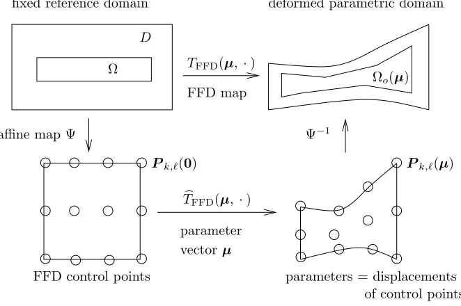
)−R0, forx1∈[0, L]. (3.6) 3.2. Free-form deformations for flexible shape parameterizations. To define the free-form deformations we assume again that there exists a reference ge-ometry Ω and look for a parametric family of smooth deformationsTFFD(µ) that can act on any kind of shape. Let Ω ⊂ D be embedded inside a control parallelogram
D, which can be mapped affinely onto the unit square, Ψ(D) = (0,1)×(0,1) with coordinates 0≤ξ1, ξ2≤1. We overlay on the unit square a regular (K+ 1)×(L+ 1) grid of control points, where the location of each control point depends only on two scalar components ofµaccording to
Pk,ℓ(µp(k,ℓ), µp(k,ℓ)+1) :=
k/K+µp(k,ℓ)
ℓ/L+µp(k,ℓ)+1
(3.7)
wherep(k, ℓ) := 2(K+ 1)ℓ+ 2k+ 1 is a condensed index into the parameter vectorµ
with a total of 2(K+ 1)(L+ 1) scalar components. Then we can define
b
TFFD(µ;ξ) := K
X
k=0 L
X
ℓ=1
a smooth, invertible “deformation of identity” mapTbFFDfor eachµin a neighborhood of0. The functionsbk,ℓare tensor products of the Bernstein basis polynomials defined as
bK,Lk,ℓ (ξ1, ξ2) :=
K
k
L ℓ
ξ1k(1−ξ1)K−kξ2ℓ(1−ξ2)L−ℓ (3.9)
for k = 0, . . . , K and ℓ = 0, . . . , L, forming a total of (K+ 1)(L+ 1) basis polyno-mials. By using the affine maps Ψ, Ψ−1 to map between the unit square and the original control parallelogram we can define the parametric free-form deformation map TFFD(µ) := Ψ−1◦Tb(µ)◦Ψ. The parametric domains are then obtained from the restriction Ωo(µ) :=TFFD(µ; Ω).
Pk,ℓ(0) Pk,ℓ(µ)
fixed reference domain deformed parametric domain
parameters = displacements FFD control points
FFD map
TFFD(µ, ·)
parameter vectorµ
Ψ−1 affine map Ψ
of control points
b
TFFD(µ, ·)
Ωo(µ) Ω
[image:8.612.91.422.250.470.2]D
Fig. 3.1.Schematic of the control points and resulting free-form parametric deformation
In Fig. 3.1 we display a schematic diagram of the free-form deformations. Using the definition and the fact that the Bernstein basis polynomials form a partition of unity it can be shown that TFFD(0) = I. Evaluation of the Bernstein basis poly-nomials (and subsequently TFFD and its Jacobian matrix) can be performed in a numerically stable fashion using the recursive de Casteljau algorithm [10] without ex-plicitly evaluating the formulas forTFFD. In case there is a need to reduce the number of geometric parameters, we can keep fixed a number of control points or only allow them to move in one dimension. This allows the user to keep the number of FFD parameters to a desired low level (in our case roughly 5-10 parameters).
4. Parametric coupling of fluid and structure. We now introduce the com-putational algorithm for the solution of the coupled fluid-structure interaction prob-lem.
equation (2.5), the trace operator Lr : V × Q → H−1/2(0, L) taking the normal component of the Cauchy stress on the interface Γw computed from the fluid residual according to (2.9), and the resolvant operatorLs:H−1/2(0, L)→ Dthat provides the structural displacement for a given applied traction. The nonlinear equation system (2.10) is equivalent to the following fixed-point problem: findη∈ Ds.t.
(I− Ls◦ Lr◦ Lf)(η) = 0. (4.1)
We can alternatively formulate the fluid-structure problem (4.1) as a minimization problem:
min
η∈D k(I− Ls◦ Lr◦ Lf)(η)k
2
D. (4.2)
Any solution of (4.1) is also a minimizer of (4.2). A simplified parametrized version of (3.5) can be given as follows: findµ∈ P that minimizes
min
µ∈P
k(I− Ls◦ Lr◦ Lf)(η(µ))k2D, (4.3)
but this time we expect that the compatibility between the traction applied by fluid and the structural displacement is only achieved in a least-squares sense. The “quality of fit” depends on the dimension of the parameter spaceP as well as the approxima-tion properties of the parametrizaapproxima-tion method. We call this theparametric coupling
approach. The parametric coupling approach was used in [35] to solve the same prob-lem, with the exception that there the applied traction (depending on this case only on the pressure profile on the wall) was directly parametrized.
Replacing the true displacement with its parametric counterpart can be under-stood as a nearest point projection step from the space of all kinematically ad-missible displacements D to the subset of parametrically admissible displacements, DP :={η ∈ D : η =η(µ),µ∈ P}, given by the operator Lp : D → DP defined as
Lp(η) := arg minη∗∈D
Pkη−η
∗k
D. We then find the equivalent formulation of (4.3)
being: findµ∈ Ps.t.
(I− Lp◦ Ls◦ Lr◦ Lf)(η(µ)) = 0. (4.4)
Remark 4.1. To prove an equivalent to Theorem 2.1 for the parametrically coupled problem, we need to adapt the Schauder fixed-point argument. This requires showing that the nearest point projection is continuous in the strongH2-norm topology.
A sufficient condition for the continuity of the parametric projection is that the set of parametric displacements DP ⊂ D be closed and convex. This is indeed the case in our FFD parametrized model problem when the parameter space P is closed and convex.
4.2. Finite element discretization of the Stokes equations. In order to give a computable algorithm for the solution of the parametrically coupled problem (4.4), we introduce discrete approximation spaces for the velocity Veh ⊂ V, pressuree
e
dim(Veh) + dim(Qeh) =Nv+Np =:Nf of the finite element spaces should be chosen large enough that for the entire parameter rangeP the finite element solution of
( e
A(ueh,veh;µ) +B(epeh,veh;µ) =F(e veh;µ)−A(egeh,veh;µ) for allevh∈Veh
e
B(eqh,ueh;µ) =−B(eqeh,geh;µ) for allqeh∈Qeh (4.5)
accurately represents the fluid solutions for the entire range of the parameter µ. While in the worst case this dictates that the finite element mesh needs to be refined uniformly everywhere, in Sect. 5 we will see that the reduced basis method alleviates the requirement of choosing a very large Nf. ByNswe denote the dimension of the structural displacement approximation space. We have corresponding bases{Ψi
v}Ni=1v, {Ψi
p}
Np
i=1, and{Ψiη}Ni=1s for each finite element space. The matrices A(µ)∈RNv×Nv,
B(µ) ∈ RNv×Np, and C ∈ RNs×Ns corresponding to the discrete operators in the
finite element basis are defined elementwise as
[A(µ)]i,j=A(Ψe jv,Ψvi;µ), [B(µ)]i,j=B(Ψe jp,Ψiv;µ), [C]i,j=C(Ψjη,Ψiη) (4.6)
and the right-hand side is given by [F(µ)]i = hF ,e Ψivi. Similarly we denote the vectorial counterparts of the variables [ue]i=ueh(xi), [pe]i=peh(xi), and [η]i=ηh(xi). We will also need the structural mass matrix M ∈ RNs×Ns defined as [M]
i,j =
RL 0 Ψ
j ηΨiηdΓ .
4.3. Parametric coupling algorithm for the discrete problem. In order to transfer the load applied by the fluid to the structure in the discrete equations, we need to construct a discrete trace operator that returns the normal component of the trace of any velocity test function on the free boundary. When the finite element spaces for the velocity and structural displacement are incompatible (because they feature either different order polynomials or they sit on nonconforming grids) one good strategy is to perform an L2-projection between the two spaces. The discrete trace operatorG:Veh→ Dhis thus defined according to
Z L
0
(Gveh)whdΓ =
Z L
0
(γΓw(evh)·n)whdΓ for allwh∈ Dh. (4.7)
In matrix form we have G:= M−1Γ, where [Γ]i,j = R L 0 (γΓw(Ψ
j
v)·n)Ψiη. This is a mortar-like approach in whichDh plays the role of slave space, see [46].
After the discrete trace operator has been formed, we can introduce a discrete version of the parametric coupled problem. Algorithm 4.1 computes a solution to the coupled problem by a fixed point iteration applied to the discretized equation (4.4). The nearest point projection is done by minimizing a least-squares functional, and involves no further fluid or structure solutions during the optimization loop. Since the analytic form (3.6) of the parametric displacement functionηh(µ) is available, the first- and second-order sensitivities are readily available, and the parametric projection step can be efficiently performed using affine-scaling interior-point Newton methods [7] for nonlinear programming with box constraints.
Algorithm 4.1Parametric coupling of fluid and structure Require: initial guess µ0
1: Letn= 0. 2: repeat
3: Solve the discretized Stokes equations foruenh=ueh(µn) andpenh=eph(µn)
4: Form the discrete fluid residual
Rh(ueh,eph;µ) =F(µn)−A(µn)
h e unh+egh
i
−B(µn)penh.
5: Form the discrete trace operatorG.
6: Solve the structural equations for the assumed displacement ηbh from Cbηh =
GRh(ueh,peh;µn).
7: Solve the constrained minimization problem in the parameter space
min
µn+1∈P h
b
ηh−ηh(µn+1)itChbηh−ηh(µn+1)i
to obtain the next configuration parameterµn+1.
8: Setn→n+ 1.
9: untilstopping criteria|µn+1−µn|<TOL is met
(Kolmogorov) N-width [40] can be used to measure the asymptotic approximation obtainable as the number of parametersP → ∞. LetX be a Banach-space endowed with norm k · kX, Y ⊂X its bounded subset whose elements we are trying to ap-proximate, and denote byXn ⊂X any linear subspace of dimension n. The optimal
N-width of the setY in the spaceX is defined as
dn(Y;X) = inf
Xn,dim(Xn)=n
sup y∈Y x∈infXn
kx−ykX (4.8)
and the spaceX∗
n that gives the infimum is the optimal subspace of dimensionn for approximatingY. In the case thatX =L2(0, L) and
Y ={y∈H2
0(0, L) : kyk2≤1} (4.9) it is known that the optimal subspace hasN-widthdn(X, Y) =λn−1/2, where 0< λ1<
λ2< . . . are the positive eigenvalues of an Euler-Bernoulli boundary-value problem: find (yk, λk)∈H02(0, L)×R+ s.t.
(y(2)k , w(2))L2 =λk(yk, w)L2 fork= 1,2, . . . . (4.10)
An optimal subspace Xn∗ is spanned by the first n eigenfunctionsyk. The N-width theory is useful in that it gives the an estimate of the worst case asymptotic con-vergence rate of an approximation to the structural displacement as the number of parametersP → ∞. The eigenvaluesλk=ℓ4k of (4.10) are solutions of (see e.g. [4])
1−(cosℓkL)(coshℓkL) = 0, (4.11)
5. Reduced basis for steady incompressible Stokes. The most computa-tionally expensive part of Algorithm 4.1 is step 3, that is, the solution of the parametric Stokes equations. With the assumption of small,C∞ geometric deformations the
de-pendence of the solutions of the Stokes equations on the parameter is also “smooth” in the sense that the manifold of parametrized solutions in the space X isC∞, and
there are no bifurcation points leading to large qualitative changes in the velocity field. With this assumption the reduced basis method can be reliably applied to reduce the problem to a much lower-dimensional subspace. The manifold of parametrized solu-tions retains its smoothness also for the Navier-Stokes equasolu-tions, provided that the Reynolds number is taken small enough. See [25, 39] for early development of the reduced basis method for Navier-Stokes equations, [6, 8, 55] for more recent results in a posteriori error estimation, and [43] for implementation details.
The reduced basis method consists of computing finite element solutions to the parametric PDEs at suitable parameter points and using their span to construct a low-dimensional approximation space for Galerkin projection. Let µ1,µ2, . . . ,µN
be a small collection of parametric configurations that form a good ensemble for approximating the behavior of the parametric fluid system in question. By computing the finite element snapshot solutions (ueh(µn),peh(µn)) s.t.
( e
A(ueh,veh;µn) +B(epeh,veh;µn) =F(e veh;µn)−A(egeh,veh;µn) for allveh∈Veh
e
B(qeh,ueh;µn) =−B(eeqh,egh;µn) for allqeh∈Qeh (5.1)
for n = 1, . . . , N we can define the problem-dependent approximation spaces for
velocity and pressure
VN
h := span(ueh(µn) : n= 1, . . . , N) QN
n := span(peh(µn) : n= 1, . . . , N)
, (5.2)
which possess some spectral approximation properties [5]. Namely, if we construct a suitably orthonormalized bases {ζnv}N
n=1 and {ζpn}nN=1 for the spaces VhN and QNn respectively and seek for a given µ ∈ P the Galerkin projection (ueNh(µn),epNh(µn)) s.t.
( e
A(ueNh,veNh;µ) +B(epeNh,ve N
h;µ) =F(e ve N
h;µ)−A(egeh,ve N
h;µ) for allve N h ∈VehN
e
B(qeNh,ue N
h;µ) =−B(eqehN,egh;µ) for allqeNh ∈QeNh (5.3) then the convergence of this reduced basis approximation, (ueNh,peNh) → (ueh,peh) as
N → ∞, is in the best case exponential inN [31] and in many applications very rapid for the entire parameter rangeµ∈ P. This means that the reduced basis dimension
N can be chosen much smaller than the finite element space dimension, N ≪ Nf, and we expect that the reduced system of sizeN×N can be efficiently assembled and solved for anyµ, and that its solution takes only negligible time and memory when compared to the cost of solving the finite element system of sizeNf× Nf. Three main aspects need to be addressed when using the reduced basis solution to approximate the underlying finite element solution:
1. Efficient methods for the assembly and solution of the reduced system (5.3). 2. Stability of the reduced basis Stokes approximation [51].
The a posteriori estimate also gives us a way to choose the parameter values{µn}N n=1 that define the RB space by a greedy algorithm that explores the parameter space [21, 49].
5.1. Efficient solution of the RB system for affine problems. The com-putational setup typical for reduced basis methods is ofoffline vs. online stages. We are willing to spend extra computational effort that depends on the (a priori large) dimension of the finite element approximation spaceNf and possibly takes consider-able time (the offline stage), provided that once the necessary data structures have been precomputed and stored, we can then assemble and solve the reduced basis sys-tem inexpensively and with complexity only depending on N, but not on Nf (the online stage) for any parametric configuration. The same requirements hold for any a posteriori error estimates we obtain in the online stage.
In reduced basis methods an important assumption that facilitates splitting the problem into offline and online stages is usually made. We say that the parametric PDE problem isaffinely parametrized if the bilinear forms satisfy
e
A(u,e ve;µ) = Qa X
q=1
Θqa(µ)Aeq(u,e ve), B(ep,e ev;µ) = Qb X
q=1
Θbq(µ)Beq(p,e ev) (5.4)
for some computable scalar functions Θa
q, Θbq depending only on the parameters, and continuous bilinear formsAeq,Beq depending only on the spatial variables, and if the linear form satisfies.
e
F(ve;µ) = Qf X
q=1
Θfq(µ)Feq(ve) (5.5)
for some computable scalar function Θf
q depending only on the parameters, and con-tinuous linear formsFeq depending only on the spatial variables. Accordingly we define the affinely decomposed matrices and right-hand sides
[Aq]i,j:=Aeq(Ψjv,Ψiv), [Bq]i,j:=Beq(Ψjp,Ψiv), [fq]j:=Feq(Ψjv). (5.6)
With assumption (5.4) the reduced basis problem splits into parameter-independent matrices and parameter-dependent scalar coefficient functions, and we obtain the linear system of 2N×2N equations to findueNh ∈RN andepN
h ∈RN s.t.
PQa
q=1Θaq(µ)ANq
PQb
q=1Θbq(µ)BNq
PQb
q=1Θbq(µ)[BNq ]t
ue
N h
e pN
h
=
f
N(
µ)
gN(µ)
, (5.7)
where the right-hand side is
f
N(
µ)
gN(µ)
:=
PQf
q=1Θfq(µ)Zvfq−
PQa
q=1Θaq(µ)ANq Zvgeh −PQb
q=1Θbq(µ)[BNq ]tZvgeh
and the reduced basis matrices and vectors are defined as
[Zv]i,j:=ζvi(xj) i= 1, . . . , N, j= 1, . . . ,Nv [Zp]i,j:=ζpi(xj) i= 1, . . . , N, j= 1, . . . ,Np
[ANq ]i,j:=ZvAqZtv, i, j= 1, . . . , N
[BNq ]i,j:=ZpBqZ t
v, i, j= 1, . . . , N
(5.9)
where the matricesZv,Zp,ANq , andBNq are assembled once and stored. The system (5.7) can then be assembled and solved for anyµ∈ Pwith complexity not depending onNf by simply evaluating the coefficient functions and summing the contributions from each term. If the affinity assumption is not in effect, the cost of the online evaluations increases and the reduced basis method becomes less attractive.
5.2. Empirical interpolation method for nonaffine problems. From the expression (3.3) for the parametric bilinear forms it is clear that the bilinear form
e
A does not satisfy the affine parametrization assumption. In fact, most geometric parametrizations are nonaffine. One way to treat nonaffinely parametrized PDEs is to use a process called the Empirical Interpolation Method (EIM) [3, 20, 30]. An approximation to the nonaffinely parametrized bilinear forms A,e B, and the lineare formFe are sought in the form
e
A(u, v;µ) = Qa X
q=1
Θaq(µ)Aeq(u,e ve) +εaEIM(x,e µ),
e
B(u, v;µ) = Qb X
q=1
Θqa(µ)Beq(u,e ev) +εbEIM(x,e µ),
e
F(v;µ) = Qf X
q=1
Θqf(µ)Feq(ve) +εfEIM(x,e µ),
(5.10)
that is, by suitable affine components plus suitable error termsεa
EIM,εbEIM,ε f EIMthat need to be controlled to an acceptable tolerance. The idea is as follows: for any scalar function g(x,µ) ∈ Cs(P;L∞(Ω)), with s ≥ 0, the goal is to find an approximate
expansion of the form
gQ(x,µ) = Q
X
q=1
Θq(µ)ψq(x) (5.11)
for whichkg(·,µ)−gQ(·,µ)kL∞(Ω)<TOL in the entire range of parametersµ∈ P.
In the empirical interpolation one seeks a set of interpolation points xq ∈ Ω and a set of shape functionsψq(x) s.t. the expansion (5.11) is obtained through solving the Lagrange interpolation problem
Q
X
q=1
[Υ]q′,q[Θ]j(µ) =g(xq ′
,µ), ∀q′ = 1, . . . , Q (5.12)
where the interpolation matrix Υ∈RQ×Qis defined elementwise as [Υ]q′,q:=ψq(xq ′
that proceeds to construct a hierarchical sequence of approximation spaces. Using the EIM for each component of [νT]i,jand combining the resulting approximate affine expansions
Ai,j
q (u,e ve) =ν
Z
Ω
ψi,jq (x)
∂uej
∂xi
∂evj
∂xi dx, forq= 1, . . . , Q
i,j (5.13)
we get
A(u,e ve;µ) = 2
X
i=1 2
X
j=1 Qi,j
X
q=1
Θi,jq (µ)Ai,jq (u,e ve) (5.14)
an expansion with a total of Qa := Q1,1+Q1,2+Q2,1+Q2,2 terms, and similarly for the other forms. In practice the EIM has been quite useful for solving nonaffinely parametrized PDEs with the reduced basis method [20, 36, 47].
Remark 5.1. For the free-form deformation detailed in Sect. 3.2 in fact the forms Be and Fe are affine due to the fact that the map TFFD is polynomial. This reduces the number of termsQa+Qb+Qf needed in the approximate affine expansion,
as was first observed in [50]. For generic nonpolynomial shape parametrizations the situation remains more challenging.
5.3. Inf-sup stability of the reduced basis Stokes approximation. We briefly recall the general existence and uniqueness theory for noncoercive linear PDEs. LetXbe a Hilbert-space endowed with the inner product (·,·)Xand the corresponding normk · kX:=
p
(·, ·)X. The general noncoercive PDE in weak form is: findU ∈X s.t.
Φ(U, V) =F(V) for allV ∈X (5.15)
where Φ :X ×X → Ris a continuous, symmetric bilinear form and F : X →R a continuous linear form. The Babuˇska inf-sup stability condition [2] that guarantees the existence of a unique solution is
∃ϕ >0 : inf U∈XVsup∈X
Φ(U, V) kUkXkVkX
≥ϕ, (5.16)
and that solution satisfies a Lax-Milgram -type stability estimate
kUkX≤ kFkX′/ϕ. (5.17)
In our Stokes case we haveU = (u, p),V = (v, q), the product spaceX :=V × Q, the norm kVk2
X := kvk2V+kqkQ2, and the bilinear form Φ(U, V) :=A(u,v) +B(p,v) +
B(q,u). The inf-sup constant ϕ in this case is the least singular value of the linear operator associated with the Stokes equation [15].
discretized problem, and thus a sufficient condition for stability is that the finite ele-ment velocity and pressure spacesVh andQhshould be chosen such that they satisfy the discrete Ladyzhenskaya-Babuˇska-Brezzi (LBB) condition [16]
∃βh>0 : inf qh∈Qh
sup
v∈Vh
B(q,v)
kvkVkqkQ ≥βh. (5.18)
Popular choices of element pairs that satisfy this condition include the mini element (P1+ bubble/P1), and the Taylor-Hood Pk+1/Pk family for k ≥ 1. In the case of parametric Stokes equations on the reference domain Ω we require further that
inf e qh∈Qeh
sup e
vh∈Veh
B(qeh,veh;µ) kevhkVekqehkQe
=βeh(µ)>0 for allµ∈ P. (5.19)
When the parametrization arises from geometric transformations and B is given by (3.3), we can use (in the case that the transform tensor is computed exactly and not approximated by numerical quadratures) the divergence of a vector field is invari-ant under the Piola transform and B(eq,eve;µ) =B(q,v), for allµ∈ P; consequently
e
βh(µ) =βh. For the reduced basis approximation we have a similar inf-sup condition
inf e qN
h∈Qe N h
sup e
vNh∈VehN
B(qeN h,ve
N h;µ) kveNhkVekqeN
hkQe
=βeNh(µ)>0 for allµ∈ P, (5.20)
but unfortunately it is not in general true that (5.19) implies (5.20). One way to guarantee stability of the reduced basis Stokes system is to enrich the velocity space with supremizers defined using the supremizer operator [51, 47]Tµ:Q
h→ Vh s.t.
(Tµqe
h,veh)Ve=B(eeqh,veh;µ) for allveh∈Veh. (5.21) Note that the name “supremizer” comes from the property
sup e
vh∈Ve e
B(qeh,veh;µ) kvehkVeh
=B(e eqh, T
µqe
h;µ) kTµqe
hkVe
. (5.22)
If for each pressure basis functionpen
h we compute the corresponding supremizer ve-locity field
e
snh(µ) :=Tµpenh (5.23)
and add these to the velocity approximation basis
e
VhN,supr(µ) :=VehN ⊕ span(es n
h(µ) : n= 1, . . . , N) (5.24)
we can replace in (5.20) the spaceVeN
h withVe N,supr
h (µ) and prove (see [51]) that now
e βN
h (µ)≥βeh(µ) so that the supremizer-enriched velocity space VehN,suprof dimension 2N inherits the inf-sup stability from the finite element problem. A difficulty related to the supremizers is that now the reduced velocity space depends explicitly on the parameter. In [51] a way to deal with this is proposed so that the explicit parameter dependence is lost. The condition βeh(µ) > 0 then implies that both ϕeh(µ) > 0 andϕeN
5.4. A posteriori error bounds for the reduced basis solution. Denoting the error between the finite element solution and its reduced basis approximation both for the velocity and pressure as eu := ueh−ueNh and ep := qeh−qehN, we denote the combined error in both velocity and pressure as
k(eu, ep)k2X:=keuk2V+kepk2Q (5.25)
and the combined residual as
Rµ(veh,qeh) :=A(eeu(µ),veh;µ) +B(eep(µ),veh;µ) +B(eqeh,eu(µ);µ) ∀(veh,qeh)∈Xh.
(5.26) ThenRµ(evh,qeh)∈Xh′ and satisfies
Rµ(evh, qh) =F(veh;µ)−A(eue
N
h,ve;µ) +B(eqehN,veh;µ) +B(eqeh,ueNh;µ) ∀(veh,qeh)∈Xh (5.27) and can be evaluated without knowing the truth finite element solution. For purposes of dual-norm computation we can define the Riesz representantbe(µ) s.t.
(be(µ),(veh,qeh))X =Rµ(veh, qh) for all (veh,eqh)∈Xh (5.28)
for whichkbe(µ)kX=kRµ(·, ·)kXh′. By applying the Babuˇska stability result (5.17)
and the inf-sup constant (5.16), we have
ϕ(µ)k(eu, ep)kX≤ sup e
v∈V,qe∈Qe
A(eu,ev;µ) +B(ep,ve;µ) +B(q,eeu;µ) k(v,e qe)kX
=kRµ(·, ·)kX′
h =kbe(µ)kX.
(5.29)
Thus for any computable lower boundϕLB(µ) for the parametric stability factor s.t. 0< ϕLB(µ)≤ϕ(µ) for allµ∈ D, the error estimator
∆N(µ) :=
kbe(µ)kX
ϕLB(µ) (5.30)
gives an upper bound for the errork(eu, ep)kX.
5.5. Estimation of the parametric stability factor. The difficulty related to the estimator (5.30) is that the definition of the parametric Babuˇska inf-sup involves the combination of two different bilinear forms AandBthat, to our knowledge, has not been as widely analyzed as the Babuˇska-Brezzi inf-sup constant, which involves only B. A successive constraint method (SCM) [24] for the construction of a lower boundϕLB(µ)>0 for the inf-sup constant was given in [22] and it works in practice also in the Stokes case. We present briefly an outline of that work with emphasis on our Stokes application (the noncoercive problem treated in the original paper was the Helmholtz equation).
First define the Babuˇska supremizer operatorTµ :X →X as the solution of
(TµU, V)
X = Φ(U, V;µ) for allV ∈X. (5.31) Note that this operator acts on the whole Stokes system whereas the supremizer operatorTµ acts only on the pressure. Similarly to the other supremizer operator it
holds that, due to (5.31), we have
sup V∈X
Φ(U, V;µ) kUkXkVkX
= Φ(U,T
µU;µ)
kUkXkTµUkX =kT
µUk
X kUkX
Note that the evaluation ofϕ(µ) at a given point can be performed by observing that in the discrete case
ϕ2h(µ) =
inf Uh∈Xh
sup Vh∈Xh
Φ(Uh, Vh;µ) kUhkXkVkX
2 =
inf Uh∈Xh
kTµU
hkX kUhkX
2 = inf
Uh∈Xh
kTµU
hk2X kUhk2X
(5.33) is a problem of finding the least eigenvalue. In matrix form the inner product is defined (Uh, Vh)X =VthXUh using a s.p.d. matrixX with Cholesky decomposition
X =HtHand thus after some computations we obtain the following matrix eigenvalue problem: find the smallestϕ2
h(µ) s.t.
H−tΦ(µ)X Φ(µ)H−1Vh=ϕ2h(µ)Vh for someVh6= 0. (5.34) The SCM was originally proposed for computing a parametric lower bound for the least eigenvalue of coercive problems that could be affinely decomposed intoQterms with complexity that is linear in Q (but depends explicitly on N and thus rather expensive). While the same could be done to find a parametric lower bound for (5.34), the operator hasQ2affine terms and the standard approach is much too cumbersome for problems with largerQ. A modification of the SCM is thus needed for noncoercive problems.
The local natural norm version of SCM for noncoercive problems seeks a lower bound for a surrogate inf-sup constant that, for a fixed parameter value ¯µ, is defined as
¯
ϕµ¯(µ) = inf U∈X
Φ(U,Tµ¯U;µ)
kTµ¯Uk2 X
. (5.35)
Values of ¯ϕµ¯(µ) are solutions of the eigenproblem (in matrix form) to find the smallest ¯
ϕµ¯(µ) s.t.
HΦ(µ)Φ−1( ¯µ)H−1Vh= ¯ϕµ¯(µ)Vh for some Vh6= 0. (5.36) Unlike the version (5.34), for ¯µfixed the operator contains only Qaffine terms. In some neighborhoodP¯µ∋µ¯ it holds thatkT
¯
µUk
X ≥CkUkX for allU ∈X, and thus thek · kX norm and the natural normkTµ¯· kX are equivalent in that neighborhood. It can be shown that ϕ( ¯µ) ¯ϕµ¯(µ) ≤ ϕ(µ) and therefore it suffices to seek a lower bound for the surrogate (5.35). This surrogate problem is coercive, so the standard successive constraint method [24] can be used. Through an iterative greedy procedure it finds a set of constraint points around which we define a set of linear constraints to find a positive lower bound for ¯ϕµ¯(µ) in the entire neighborhoodPµ¯. When this is
performed for sufficiently many ¯µthe sets P¯µ cover the entire parameter range and
we can compute a parametric lower bound for ϕ(µ) accordingly. For details of the local lower bound construction for ¯ϕµ¯(µ) inPµ¯, we refer to [22].
OFFLINE
ONLINE
Solution Basis selection by greedy algorithm
Affine decomposition Successive constraint
∆N(µ)
AN(µ), BN(µ), fN(µ)
and assembly method
Assembly
ΦN(
µ)UN(µ) =fN(µ)
ϕLB(µ)
A posteriori estimator STAGE
STAGE
Aq, Bq, fq
Zv, Zp, A N q, B
N q, f
N q
Certified RB solution
UN(
[image:19.612.118.394.86.344.2]µ),∆N(µ)
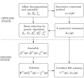
Fig. 5.1. Schematic description of the offline and online stages of the RB method. All the structures created in the offline stage are independent ofµ, and thus are computed once and stored
in preparation for the online stage. The online stage is independent of the truth FEM dimensionN once these structures have been precomputed.
dependent onN, but also magnified by a factor relating to the inherent complexity of the parametrization as codified by the number of affine terms Qb. As is typical for offline-online reduction schemes, the cost of the offline stage is therefore orders of magnitude larger than the cost of one finite element solution of the parametric PDE.
Once the inf-sup lower bound has been constructed, the estimator (5.30) is used to drive a greedy algorithm [21], such as the one detailed in Algorithm 5.1. The al-gorithm selects hierarchically the velocity and pressure basis functions by adding at each iteration the worst approximated element of a finite training set according to the error estimator (5.30), computes the supremizer (5.23) and adds it to the velocity basis, and performs an orthonormalization of the basis to improve the algebraic con-ditioning of the small but full linear system (5.7). Finally, the reduced order matrices and right-hand sides (5.9) are computed and stored. With the assumption of affine parameter dependence, the computation of the residual (5.28) in the a posteriori es-timator can be treated with a similar offline-online procedure. In matrix form we can write the vectorsUNh(µ) andVNh(µ) in the reduced basis expansion
UNh(µ) = N
X
n=1
UnN(µ)ζnU, VNh(µ) = N
X
n=1
so that the residual can be affinely decomposed
R(V;µ) = Qf X
q=1
Θfq(µ)Fq(V)− Q
X
q=1
ΘΦq(µ)Φq(UhN, V)
= Qf X
q=1
Θfq(µ)Fq(V)− N
X
n=1
uNn(µ) Q
X
q=1
ΘΦq(µ)Φq(ζUn, V)
, (5.38)
which together with (5.28) implies
b e(µ) =
Qf X
q=1
Θfq(µ)Cq− N
X
n=1
uNn(µ) Q
X
q=1
ΘΦq(µ)Lnq (5.39)
where (Cq, V)X =Fq(V) for allV ∈Xh and (LNq , V)X = Φ(ζUn, V) for allV ∈Xh. Then
kbe(µ)k2X= Qf X
q=1 Qf X
q′=1
Θfq(µ)Θ f
q′(µ)(Cq, Cq′)X
− Q X q=1 N X n=1
uNn(µ)ΘΦq(µ)
2
Qf X
q=1
Θfq(µ)(Cq, Lnq)X− Q
X
q′=1
N
X
n′=1
uNn′(µ)ΘΦq′(µ)(Lnq, Ln ′
q′)X
(5.40) The inner products (Cq, Cq′)X, (Cq, Ln
q)X, (Lnq, Ln
′
q′)Xcan be precomputed at the end
of the offline stage and stored in the offline stage once the reduced basis{ζn
U}Nn=1 has been selected. In the online stage the norm of the residual can then be evaluated from the formula (5.40) for eachµwith complexity only involvingN.
6. Numerical results. To demonstrate the reliability of the RB method for the parametrized Stokes equations, we used a simplified FFD parametrization with
P = 2 parameters. The reference domain Ω = (0,3)×(−1,0) represents a half-width of the actual channel owing to symmetry, and its radius was taken as R0 = 0.5 cm. The free-form deformation used a 4×2 regular grid of control points, where only the 2 central points on the upper row were allowed to move freely in the x2-direction. In Fig. 6.1(a) we present the resulting deformed image of the reference domain in two different parameter configurations overlaid with the corresponding positions of the control points. For the Stokes problem using P2/P1-elements this mesh gives a total of Nf = 7940 degrees of freedom. We choose to refine locally the mesh near the free boundary Γw and the outlet Γout, since in our experience these parts yield the largest contribution to the error in the reduced basis approximation of the Stokes equations. The viscosity was chosen as the physiological valueν = 0.035 g/cm·s, and the parabolic inflow velocityg(x2) =30(1−(1 +x2)2) 0tcm/s.
The transformation tensors (3.1) and (3.2) were computed symbolically using a Computer Algebra System (CAS). The empirical interpolation procedure was used to obtain an affinely parametrized version of the Stokes equations on the reference domain. The transformation tensor elements were evaluted by the CAS and the EIM procedure was used to obtain an affine approximate expansion for each tensor compo-nent separately. With a stopping tolerance of 1e-5 in theL∞-norm the total number
Algorithm 5.1Greedy reduced basis selection Require: Large training sample ΞRB
train ⊂ P, initial snapshot parameter valueµ1
1: Letn= 1.
2: Set the first reduced basis vectors ζ1 v = e
uh(µ1)
kuhe (µ1)kVe, andζ
1 p = e
ph(µ1)
kpeh(µ1)kQe
3: repeat
4: Compute (Cq, Lnq)X and (Lnq, Ln
′
q′)X forn′ = 1, . . . , nand q= 1, . . . , Q needed
to evaluate ∆n(µ) via (5.40).
5: Choose next parameter using the estimatorµn+1= argmaxµ∈ΞRBtrain ∆n(µ
n+1). and compute the corresponding snapshot FE solution (ueh(µn+1),eph(µn+1)).
6: Compute the next supremizer by solvingXs(µn+1) =B(µn+1)peh(µn+1).
7: Orthonormalize to get the next basis vectors and supremizers
zvn+1=ueh(µn+1)− n
X
n′=1
ζvn′(ueh(µn+1), ζn
′
v )Ve
zpn+1=peh(µn+1)− n
X
n′=1
ζpn′(peh(µn+1), ζn
′
p )Qe
ζn+1
v =
zn+1 v kzvn+1kVe
, ζn+1
s =
sn+1 ksn+1k
e
V ,
8: until∆n(µn+1)≤TOL
0 0.5 1 1.5 2 2.5 3
−1 −0.8 −0.6 −0.4 −0.2 0 0.2
(a)
0 0.5 1 1.5 2 2.5 3
−1 −0.8 −0.6 −0.4 −0.2 0 0.2
[image:21.612.73.443.168.480.2](b)
Fig. 6.1. Two different parametric configurations ofΩo(µ) induced by the FFD in case (a)
P = 2 and (b) P = 10. Positions of control points in the reference and deformed configurations marked in by◦.
also be possible to derive by hand the affine decompositions, nevertheless, to be consis-tent in treating the different coefficient functions we used the empirical interpolation method on both parts. When the EIM is applied to an affinely parametrized function it simply stops after a finite number of steps as the error drops to zero (up to machine precision).
6.1. Reduction of the parametric Stokes problem withP = 2. After the flow channel has been parametrized with FFDs and the affinely parametric decom-position of the problem has been achieved using the EIM, we can apply the reduced basis machinery. Using the same parameter range as for the EIM,µ1, µ2∈[−0.1,0.1], we used the SCM to compute a lower bound for the parametric Babuska inf-sup con-stant ϕLB(µ). It turns out that for this parametrization the SCM only needed one
¯
−0.1 −0.05
0 0.05
0.1
−0.1 −0.05 0 0.05 0.1 0.2 0.3 0.4
µ 1 µ
2
Inf−sup lower bound given by the SCM 0.2 0.22 0.24 0.26 0.28 0.3 0.32 0.34 0.36
(a)
−0.1 −0.05
0 0.05
0.1
−0.1 −0.05 0 0.05 0.1 0.2 0.3 0.4
µ1
µ 2
Inf−sup upper bound given by the SCM 0.2 0.22 0.24 0.26 0.28 0.3 0.32 0.34 0.36
[image:22.612.85.421.107.248.2](b)
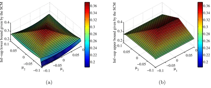
Fig. 6.2.Successive constraint method obtained (a) lower bound surfaceϕLB(µ)and (b) upper
bound surfaceϕUB(µ)for the parameter-dependent Babuska inf-sup constant
training sample up to the acceptable tolerance for the bound gap, i.e.
ϕUB(µ)−ϕLB(µ)
ϕUB(µ) ≤0.25 for allµ∈Ξ SCM
train. (6.1) In Fig. 6.2 we present the online lower bound estimate ϕLB(µ) and upper bound estimate ϕUB(µ) computed for the entire parameter range. The lower bound is ev-erywhere positive, and therefore the SCM can be deemed to have been successful.
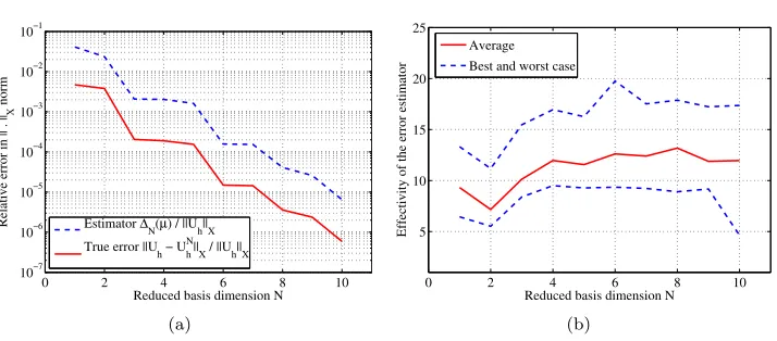
Using the a posteriori estimate (5.30) and the greedy Algorithm 5.1 for basis selection, a total of Nmax = 10 basis functions were chosen to satisfy the tolerance ∆N(µ) < 1e-5 for all µ ∈ ΞRBtrain. After the necessary online structures have been computed, we compare the (affinely decomposed2) finite element “truth solution” to the reduced basis approximation using a variable numberN = 1,2, . . . , Nmaxof basis functions. In Fig. 6.3(a) we display the true error and compare it to the a posteriori estimator ∆N(µ) for one typical parameter value (in this caseµ= [0.1,−0.1]). The convergence is rapid, if not quite exponential, and the gap between the true error and the a posteriori estimator remains more or less the same for allN. In the other plot we show the effectivity of the error estimator
ϑ(µ) := ∆N(µ)
kUh(µ)−UhN(µ)kX
(6.2)
over a random sample of 1000 different parameter points both as an average over the entire sample as well as the best- and worst-case bounds. For a rigorous upper bound we must haveϑ≥1 and to have an efficient upper bound we demand thatϑremains bounded forN → ∞. From Fig. 6.3 we see that the obtained bounds in this case are both rigorous and efficient.
6.2. Reduction of the parametric Stokes problem with P = 10. To test the parametric coupling Algorithm 4.1 we introduced a different FFD parametrization with P = 10 parameters. This time we used a 14×2 regular grid of control points,
2
0 2 4 6 8 10 10−7
10−6 10−5 10−4 10−3 10−2 10−1
Reduced basis dimension N
Relative error in || . ||
X
norm
Estimator ∆
[image:23.612.79.436.92.249.2]N(µ) / ||Uh||X
True error ||U
h − Uh N
||
X / ||Uh||X
(a)
0 2 4 6 8 10
5 10 15 20 25
Reduced basis dimension N
Effectivity of the error estimator
Average
Best and worst case
(b)
Fig. 6.3. Case P = 2: (a) Relative error between reduced basis solution Un
h and truth FEM solution Uh and the corresponding error estimate ∆N(µ) for one parameter value µ ∈ P; (b)
Effectivity of the a posteriori error estimator∆N(µ)over a sample set of 1000 different parameter
values for different reduced basis dimensionsN
where only the 10 central points on the upper row were allowed to move freely in the
x2-direction. In Fig. 6.1(b) we present the resulting deformed image of the reference domain in two different parameter configurations overlaid with the corresponding positions of the control points. Again the two left- and rightmost columns of control points were kept fixed. Using a stopping tolerance of 1e-4 in the L∞-norm for the EIM, the total number of affine terms wereQa = 68 for viscous part the andQb= 22 for the pressure-divergence part. As we can observe, the number of affine terms grows considerably as a function of the number of FFD parameters P. The acceptable parameter range was againµp ∈[−0.1,0.1] forp= 1,2, . . . ,10. The discretization of the Stokes problem remained the same.
The natural norm SCM algorithm converges very slowly when the number of parameters is larger than P ≤ 3. Thus for the setup with P = 10 we were not able to obtain a lower bound estimate in a similar fashion. We however observe that for the channel problem adding more free-form parameters does not affect the range of stability factors ϕ−1(µ). In fact, in [56] it was demonstrated that for a periodic channel the Brezzi inf-sup constant β(µ) (which is related to the Babuˇska inf-sup constant, see e.g. [48]) depends mostly on the width of the narrowest part of the channel. Thus we circumvented the problems related to the SCM by using a global constant,ϕLB= 0.185 for allµ∈ D, as the lower bound. This was obtained according to Fig. 6.2(a) from the caseP = 2. The greedy Algorithm 5.1 for basis selection was driven to select a fixed number of Nmax = 30 basis functions. In Fig. 6.4 we show as before the error estimate and its effectivity over a random sample of 1000 different parameter points. Despite the rather pessimistic bound for the parametric stability factor the resulting estimator still has reasonable effectivity. The relative error of the reduced Stokes solutions is slightly larger than in the previous case, but still less than 0.1%.
0 5 10 15 20 25 30 10−5
10−4 10−3 10−2 10−1 100 101
Reduced basis dimension N
Relative error in || . ||
X
norm
[image:24.612.80.436.102.248.2] [image:24.612.84.439.442.577.2]Estimator ∆ N(µ) / ||Uh||X True error ||U
h − Uh N ||
X / ||Uh||X
(a)
0 5 10 15 20 25 30
100 200 300 400 500 600 700
Reduced basis dimension N
Effectivity of the error estimator
Average Best and worst case
(b)
Fig. 6.4. CaseP = 10: (a) Relative error between reduced basis solution Un
h and truth FEM solution Uh and the corresponding error estimate ∆N(µ) for one parameter value µ ∈ P; (b)
Effectivity of the a posteriori error estimator∆N(µ)over a sample set of 1000 different parameter
values for different reduced basis dimensionsN
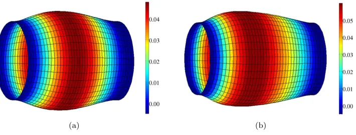
solved using the full finite element model. The physical parameters of the structural equations were chosen asE= 0.75·106 dyn/cm2,h= 0.1 cm, ν
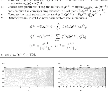
P = 0.5,K= 0.9643, and G= 0.20·106 dyn/cm2 according to [12]. The fourth order perturbation term was chosen according to two different values, ε= 1e-2 and ε = 1e-3. In the former case the shape of the deformed tube is closer to being symmetric, while in the latter case we obtain a highly unsymmetric deformed shape due to the reduced stiffness of the wall and the pressure profile imposed by the mixed boundary conditions. In Fig. 6.5 we display a visualization of the displacement of the structure at the end of the coupling iteration in both of the aforementioned cases.
(a) (b)
Fig. 6.5. Visualization of the displacement of the structure of the coupled solution (displace-ments magnified) for (a)ε= 1e-2 and (b)ε= 1e-3.
measure the coupling accuracy. In this case after the final iteration we obtained
kη(µk)−ηb(µk)k
kη(µk)k = 1.112e-3 (6.3) The prototype code was written in Matlab and ran serially on one Intel Xeon 2.40 GHz processor with 4 GB of working memory. In this case the coupled solution was obtained in 580 s with the reduced fluid equations, and in 630 s with the full finite element fluid equations. The rather small difference is due to several factors. A partitioned procedure that subiterates between fluid and structure solves is usually computationally more expensive than a monolithic procedure that solves directly the coupled nonlinear fluid-structure system. Only one fluid solve is needed on each major iteration of the partitioned algorithm, while the rest of the work is done to minimize the least squares difference between the structural deformation and the parametric deformation of the geometry. The latter part does not currently benefit from the reduction by reduced basis and can dominate the computational cost, especially when a small coupling tolerance was requested. This reduced considerably the computa-tional savings related to the partitioned procedure. The fixed point iteration was also employed as is, whereas an accelerated fixed point method [9] or a Newton method would considerably improve the convergence rate. Together with the implementation of the nonlinear Navier-Stokes equations for the fluid these are future improvements. In any case, the reduced systems of size 30×30 are small enough to be used as part of a very large flow network consisting of hundreds of coupled FSI elements.
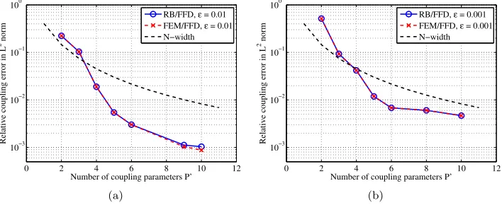
To test the coupling accuracy obtained using a different number P′ of free-form
deformation parameters we defined a monotonically increasing subset of the parame-ters forP′= 2,3,4,5,6,7,8,9, where the rest of the parameters were fixed atµ
p= 0 in each case. The coupled solution was then computed in each of these cases. In Fig. 6.6 we display the relative error of the final displacement for different values of
P′ forε = 1e-2 andε= 1e-3, both computed with the reduced fluid equations and the full FEM. The coupling accuracies obtained by using RB and FEM were virtu-ally the same. The theoretical optimalN-width was computed from (4.11). In both cases the coupling accuracy converges at least as fast as the worst-case asymptotic rate predicted by the N-width theory. We read this as an indication that the FFD parametrization is suitable for the problem at hand and allows the user to achieve desired coupling accuracy by selecting the number of FFD parametersP large enough.
7. Conclusions and future work. We have presented a new approach to model reduction of a coupled fluid-structure interaction problem. By introducing a paramet-ric free-form deformation of the flow geometry the fluid equations can be written as parametric partial differential equations on a fixed domain. We then applied the reduced basis method to the fluid equations to obtain an efficient reduced model with certified error bounds. The geometric deformation parameters were also used to couple the fluid domain to a 1-d wall equation, where the parameters acted as the coupling variables. We demonstrated that for a modest number of free-form de-formation parameters an approximate coupling between fluid and structure can be achieved. The same coupling accuracy was achieved for both the full finite element fluid model and the reduced model withN = 30 basis functions. Future work involves extending the approach to the unsteady case and coupling the individual reduced basis fluid-structure models into a large flow network.
contri-0 2 4 6 8 10 12 10−3
10−2 10−1 100
Number of coupling parameters P’
Relative coupling error in L
2 norm
RB/FFD, ε = 0.01 FEM/FFD, ε = 0.01 N−width
(a)
0 2 4 6 8 10 12
10−3 10−2 10−1 100
Number of coupling parameters P’
Relative coupling error in L
2 norm
RB/FFD, ε = 0.001 FEM/FFD, ε = 0.001 N−width
[image:26.612.80.434.103.248.2](b)
Fig. 6.6. RelativeL2
-errorkη−ηk/kηkb at the end of Algorithm 4.1 for (a)ε= 1e-2 and (b) ε= 1e-3. The theoreticalN-width is computed according to (4.11).
butions on the Stokes part. Numerical simulations were based on the rbMIT toolkit [23] developed by the group of Anthony Patera as well as the MLife fluid mechanics solvers originally authored by Fausto Saleri.
REFERENCES
[1] B.O. Almroth, P. Stern, and F.A. Brogan,Automatic choice of global shape functions in structural analysis, AIAA J., 16 (1978), pp. 525–528.
[2] I. Babuˇska and A.K. Aziz,Lectures on the mathematical foundations of the finite element method, Tech. Report BN-748, University of Maryland, College Park, Washington DC, 1972.
[3] M. Barrault, Y. Maday, N.C. Nguyen, and A.T. Patera, An ‘empirical interpolation’ method: application to efficient reduced-basis discretization of partial differential equations, C. R. Math. Acad. Sci. Paris, 339 (2004), pp. 667 – 672.
[4] H. Bremer,Elastic multibody dynamics: a direct Ritz approach, Springer Science+Business Media, 2008.
[5] C.G. Canuto, M.Y. Hussaini, A. Quarteroni, and Th.A. Zang,Spectral Methods: Evolution to Complex Geometries and Applications to Fluid Dynamics, Springer, 2007.
[6] C. Canuto, T. Tonn, and K. Urban,A posteriori error analysis of the reduced basis method for nonaffine parametrized nonlinear PDEs, SIAM J. Numer. Anal., 47(3) (2009), pp. 2001– 2022.
[7] T. F. Coleman and Y. Li, An interior trust region approach for nonlinear minimization subject to bounds, SIAM J. Optimization, 6 (1996), pp. 418–445.
[8] S. Deparis, Reduced basis error bound computation of parameter-dependent Navier–Stokes equations by the natural norm approach, SIAM J. Num. Anal., 46 (2008), pp. 2039–2067. [9] S. Deparis, M.A. Fern´andez, and L. Formaggia,Acceleration of a fixed point algorithm for fluid-structure interaction using transpiration conditions, ESAIM Math. Modelling Numer. Anal., 37 (2003), pp. 601–616.
[10] G. Farin,Curves and surfaces for computer-aided geometric design: a practical guide, Morgan Kaufmann, 2001.
[11] J.P. Fink and W.C. Rheinboldt,On the error behavior of the reduced basis technique for nonlinear finite element approximations, Z. Angew. Math. Mech., 63(1) (1983), pp. 21–28. [12] L. Formaggia, J.-F. Gerbeau, F. Nobile, and F. Quarteroni,On the coupling of 3D and 1D Navier-Stokes equations for flow problems in compliant vessels, Comput. Methods Appl. Mech. Engrg., 191(6-7) (2001), pp. 561–582.
[13] L. Formaggia, A. Quarteroni, and A. Veneziani,Multiscale models of the vascular sys-tem, In: Formaggia, L.; Quarteroni, A; Veneziani, A. (Eds.), Cardiovascular Mathematics, Springer, (2009).