White Rose Research Online URL for this paper:
http://eprints.whiterose.ac.uk/88836/
Version: Accepted Version
Article:
Kim, J orcid.org/0000-0002-3456-6614 and Cho, K-H (2016) Robustness analysis of
network modularity. IEEE Transactions on Control of Network Systems, 3 (4). 16561944.
pp. 348-357. ISSN 2325-5870
https://doi.org/10.1109/TCNS.2015.2476197
© 2015, IEEE. Uploaded in accordance with the publisher's self-archiving policy. Personal
use of this material is permitted. Permission from IEEE must be obtained for all other
users, including reprinting/ republishing this material for advertising or promotional
purposes, creating new collective works for resale or redistribution to servers or lists, or
reuse of any copyrighted components of this work in other works.
[email protected] https://eprints.whiterose.ac.uk/ Reuse
Unless indicated otherwise, fulltext items are protected by copyright with all rights reserved. The copyright exception in section 29 of the Copyright, Designs and Patents Act 1988 allows the making of a single copy solely for the purpose of non-commercial research or private study within the limits of fair dealing. The publisher or other rights-holder may allow further reproduction and re-use of this version - refer to the White Rose Research Online record for this item. Where records identify the publisher as the copyright holder, users can verify any specific terms of use on the publisher’s website.
Takedown
If you consider content in White Rose Research Online to be in breach of UK law, please notify us by
Robustness analysis of network modularity
Jongrae Kim,
Member, IEEE
, and Kwang-Hyun Cho,
Senior Member, IEEE
Abstract—Modules are commonly observed functional units in large-scale networks and the dynamics of networks are closely related to the organization of such modules. Modularity analysis has been widely used to investigate the organizing principle of complex networks. The information about network topology needed for such modularity analysis is, however, not complete in many real world networks. We noted that network structure is often reconstructed based on partial observation and therefore it is re-organized as more information is collected. Hence, it is critical to evaluate the robustness of network modules with respect to uncertainties. For this purpose, we have developed a robustness bounds algorithm that provides an estimation of the unknown minimal perturbation, which breaks down the original modularity. The proposed algorithm is computationally efficient and provides valuable information about the robustness of modularity for large-scale network analysis.
Index Terms—Network modularity, community structure, ro-bustness analysis
I. INTRODUCTION
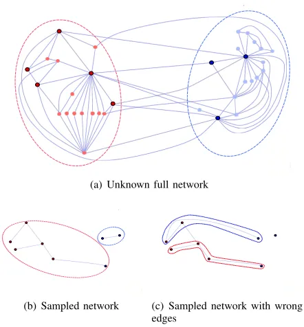
Network or graph theory has been applied to modelling many physical, biological, and social systems for various interaction data such as internet communications, biomolecular interactome, and social relationships. A network consists of nodes and edges as shown in Fig.1(a), where a node may represent a computer server in the internet, a protein species in a protein-protein interaction network, or an individual person in a social network, and an edge may denote a physical network connection between two computers, a protein-protein interaction between the protein species, or friendship between two people. Because of the simplicity of network modelling, a massive number of components and interactions can be considered easily for many cases.
The most important finding in large-scale network analysis is arguably the scale-free characteristic [1]. This explains two important properties, i.e., robustness and small-worldness, in large-scale networks. Another important way of compre-hending large-scale networks is modularity analysis, which has been one of academic research interest in recent years. There are several different definitions on network modularity [2], [3], [4], [5], [6]. Among these, a defining characteristic of a module is that nodes in the same module have more frequent interconnections than to the connections to the nodes in different modules. The formulation proposed by Newman [2] is one of the widely accepted definitions as it shows a quite intuitive result and the module calculation can be done efficiently using the power iteration. The community or
J. Kim is with the School of Mechanical Engineering, University of Leeds, Leeds LS2 9T, UK, Tel. +44(0)113 343 2159, E-mail: [email protected]. K.-H. Cho, Corresponding Author, is with the Department of Bio and Brain Engineering, Korea Advanced Institute of Science & Technology (KAIST), Daejeon 305-701, Republic of Korea, Tel. +82(0)42 350 4325, E-mail: [email protected]
(a) Unknown full network
[image:2.612.329.550.142.380.2](b) Sampled network (c) Sampled network with wrong edges
Fig. 1. Modularity and sampling effects: (a) Eight darker nodes are sampled for (b) and (c); (b) One node is categorized in the wrong module; (c) The thick gray edge is incorrectly identified, and one edge and one node are not observed.
modular structure provides us with the information about the hidden functional organization of the networks. For instance, two modules indicated by the ellipsoids in Fig.1(a) indicate that social division occurred in a Karate club in America [7], where the network shows the friend-relationships among the club members.
A profound consequence of the modular structure of com-plex networks is the enhanced robustness to various internal and external perturbations and disturbances. Robustness is considered to be one of the key factors that shaped biolog-ical systems through evolution. Modular system design is an efficient way to distribute and organize functions as frequently observed in many engineering systems, whose design evolves as well based on their performance. The functional modu-larization might be the origin of robustness [8] and highly optimized tolerance [9]. In addition, graph partition is an important control problem to organize multiple agents in order to perform a common mission while communications among them are limited [10].
A number of previous studies reported how to dissect hierarchical modular structures [1] and interpret their physical, biological and social meanings [1], [11], [12].
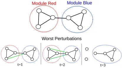
Module Red Module Blue
Worst Perturbations
[image:3.612.71.278.52.167.2]t=1 t=2 t=3
Fig. 2. A simple network and its worst case perturbation for each number of edge alterations (t).
a snap shot at a fixed time. For instance, we may not have the full network data as shown in Fig.1(a) but only have the partial sampling such as Fig.1(b) or 1(c). As the available network data are only a partial subset of the unknown true network, the modular structure inferred from such data would be influenced by the sampling effect as illustrated in Fig.1(b), where one node is included in a wrong module. In addition, a sampled network might include a false interaction, e.g. the gray edge in Fig.1(c) (false positive) or miss a true edge between one of the blue nodes and the lighter blue nodes (false negative). This sampling effect was reported in the past. For example, identifying high degree nodes in different categories of biological networks [11] cannot be supported from the data used [13] and the power-law degree distribution in scale-free networks is highly sensitive to the data analyzed [14]. Hence, any network modularity analysis needs to be further validated by robustness analysis with respect to the network uncertainty in terms of false positive or negative nodes and edges.
To examine the effect of such uncertainties on the modular-ity structure, we need to identify the minimal perturbation that can break down the original modularity of the network. For instance, a simple six-nodes network shown in Fig. 2 can be divided into two modules, the red and the blue. By applying all possible perturbations, we find that removing three edges shown in Fig. 2 is the minimum number of edge perturbations, which destroys the original modularity. Based on this minimal perturbation, we can measure the robustness of the current modular structure. The number of possible perturbations to be examined for an exhaustive search increases exponentially along with the size of a network and therefore it is impossible to perform a full search even for a network of a moderate size. This paper is organized as follows. First, the robustness analysis is formulated as a quadratic integer programming problem. Second, the upper and lower bound algorithms are established. Third, the algorithms are applied to various ex-ample networks including a social network, the yeast protein-protein interaction (PPI) network, and a research citation network. Finally, conclusions are made.
II. ROBUSTNESS OF MODULARITY
An n×nadjacency matrix,A, describes a network withn number of nodes, where thei-H row andj-th column of the matrixAis set to 1 if the two nodes are directly connected or 0 if there is no direct connection. The solution of the following
maximization problem [2],
Maximize
s∈S Q(
s, A) := 1
4ms
TBs, (1)
dividesn nodes in Ainto two groups for Q >0 or declares the network indivisible for Q≤ 0, where S is the set of
n-dimensional column vectors,s, whose element is either 1 or -1, mis the number of edges in the network,(·)T is the transpose,
k=A1, each value inkis called the degree of node,1is the n-dimensional column vector whose elements are all 1, and
B:=A−kk
T
2m .
B measures the difference between the current edge distri-bution,A, and the average edge distribution,kkT/(2m). The maximum value ofQbeing positive indicates more edges than expected in each subgroup for a division given bys, and the nodes are separated into two groups depending on the sign of elements ins.
With the optimal solution to (1) denoted bys∗
, the maxi-mum modularity,Q∗
, is given by
Q∗
= max(Q) =Q(s∗
, A).
WhileAis fixed in the maximisation problem, in reality, the network is most likely a subset of the unknown true network including some false positive or false negative edges/nodes, and it might even change with time. For brevity, only the edge perturbation case is considered and the general case including node perturbation will be discussed at the end. Once edges are added to and/or removed from the current network, the adjacency matrix is changed.
Ag :=A+ ∆A,
where the subscript g represents the perturbed network, ∆A
isn×n matrix representing removal (-1) or addition (+1) of edges to the original network. The perturbedB is given by
Bg:=Ag−
1 2mg
kgkTg,
kg:=Ag1=k+δk,
mg is the number of edges in the perturbed network, 1 is
assumed to have an appropriate dimension from now on, and δk is an n-dimensional vector, whose elements represent the
degree changes of the nodes in the network. he robustness analysis problem is formulated as follows:
Problem 1: (Robustness analysis of modularity) For a given network,A, and the partition,s∗
, find∆A minimisingQg as
follows:
Minimize
∆A
Qg(s∗,∆A)
for a fixed number of alterations, t ∈[1,min(t1, t2)], where Qg(s∗,∆A) :=Q(s∗, Ag),t1=mandt2=n(n−1)/2−m.
For each number of alterations,t, the worst perturbation,∆A,
connected. The upper bound oftcorresponds to either one of these two extreme cases. It can be shown that the following is equivalent toProblem 1:
Problem 2: (Robustness analysis of modularity) Fortin the range of [1,min(t1, t2)], find dv such that
Minimize
dv∈Dv q(
dv) =a·dv−(b·dv) 2
b , (2)
whereDv is the set of all feasible column vectors,dv, whose dimension is n(n−1)/2 and the value of each element is 0 (no change) or 1 (either remove the edge if an edge exists or add an edge if not).dv is constructed by vectorizing∆Aand dT
v1 =t. “·” is the dot product, a andbare vectors, which
are constructed fromA,m, ands∗
, andbis the magnitude of b(see Appendix for the full definitions).
Proof: See Appendix.
Once the minimization problem is solved, the worst Qg is
calculated as follows:
Qworst
g (t) := min α∈Sα(t)Qg
= min
α∈Sα(t)
(
1 1 +α
"
Q∗
+ α(k·s
∗
)2 8m2(1 +α)+
q∗
4m
#)
,
whereq∗
is the minimum ofq(dv),αis given by
2mg=1TAg1= 2m(1 +α),
andSα(t)is the set of all possible elements ofαfor a fixed
t as follows:
Sα(t) =
(
{0,±2/m,±4/m, . . . ,±t/m} for tis even,
{±1/m,±3/m, . . . ,±t/m} fort is odd. α is the net number of edge alterations. Positive or negative values ofαimply that after perturbation the number of edges in A has increased or decreased, respectively. For a fixed number of alterations,t, there is more than one possible value of αgiven by the setSα(t).
Modularity robustness analysis is presented as a quadratic integer programming problem. The computational cost in-creases exponentially as fast asPn
k=1n!/[k!(n−k)!]. Calculat-ing the exact solution requires unreasonable computation time for even some moderate size problems. Hence, developing an efficient lower and upper bounds algorithm is greatly desirable. However, we note that any bounds algorithm will eventually produce conservative results for some cases, which is the unavoidable risk for using bounds algorithms.
A. Robustness lower bound
By the definition of vector dot product, the minimization problem, (2), can be written as
Minimize
dv∈Dv q(
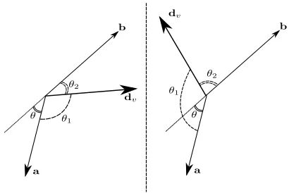
dv) =advcosθ1−bd2vcos2θ2 (3) subject to dv·1=t, wheret ∈[1,min(t1, t2)], aand dv is the magnitude of a anddv, respectively. The angle between
a and dv is θ1, while the angle between b anddv is θ2. It can be shown thatθ1 is in the following range:
cos−1
P i∈M¯ ai
a√t
≤θ1≤cos−1
P i∈Mai
a√t
!
,
whereM¯ andM are the sets, whose elements are the indices of the first t-number of largest and smallest elements in a, respectively.θ2 is equal toπ+θ−θ1 forθ+θ1+θ2> π or π−θ−θ1 otherwise (See Proposition A.1 in appendix). The minimizingq(dv)is shown to be equivalent to:
Minimize
θ1∈[θ1,θ¯1]
q(θ1) =a√tx−bt(xcosθ±p1−x2sinθ)2, and the minimum of q(θ1) occurs at x∗
, which is either the solution of quartic equation, i.e., P4
i=0wixi = 0, where
x = cosθ1, or one of the boundary values for θ1, i.e., x = cosθ1 or x = cos ¯θ1 . The definitions of wi and the
proofs are shown in Propositions A.2 and A.3 in appendix. All solutions of the quartic equations for x can easily be calculated and the minimum solution, θ∗
1, is given by
cos−1x∗
. Now, we are ready to present a lower bound algorithm.
Theorem 2.1: (Lower Bound) For a givent, the worst case, Qworst
g (t), is bounded below by
QLB[α∗LB(t)]≤Qworstg (t),
whereα∈Sα(t),
QLB(α) :=
1 1 +α
"
Q∗
+ α(k·s
∗
)2 8m2(1 +α)+
q(θ∗
1)
4m
#
,
α∗
LB(t) = argmin α∈Sα(t)
QLB(α).
Proof: By the definition, q(θ∗
1) is less than or equal to q
∗
, and it leads toQLB[α∗LB(t)]≤Q
worst
g (α).
In order to find the lower bound, first, calculate minq(θ1)
for allα∈Sα(t), second, substitute these intoQLB(α), take
the minimum among QLB(α) for α ∈ Sα(t), and finally,
repeat these for differenttvalues. This algorithm requires only polynomial computation time.
B. Robustness upper bound
Whether the lower bound is close to the true worst or not can be verified by an upper bound. To develop an upper bound, the following inequality is derived:
min
dv∈Dvq(
dv)≤q(¯dv),
whered¯v represents some specific perturbation, ∆A, defined by Proposition A.4 in appendix. The next step is to solve the following minimization problem, which is constructed from q(dv)shown in Proposition A.4:
Minimize
dv∈Dv p(
This is only a function ofdv excludingα. Expand the vector multiplications,
p(dv) =a1dv1+a2dv2+. . .+aldvl
−˜b1dv1+ ˜b2dv2+. . .+ ˜bldvl 2
,
where ai, ˜bi and dvi are the i-th element of (aT1 −a˜T2)Av,
˜
b and dv, respectively, for i = 1,2, . . . , l − 1, l, and l=n(n−1)/2. Notice thatd2
vi=dvi asdviis either 0 or 1.
For brevity, consider n= 3 case, the formulations for the general cases can be derived similarly.
p(dv) =c1dv1+c2dv2+c3dv3
−2˜b1˜b2dv1dv2−2˜b1˜b3dv1dv3−2˜b2˜b3dv2dv3,
where ci =ai−˜b2i for i= 1,2,3. Again, this is a quadratic
integer programming problem. Although any perturbation will provide an upper bound, in order to reduce the unknown distance from the worst case and simplify the calculations, p(dv)is modified as follows:
ˆ
p(ˆdv) =c1dv1dv2+c1dv1dv3+c2dv1dv2+c2dv2dv3
+c3dv1dv3+c3dv2dv3−2˜b1˜b2dv1dv2
−2˜b1˜b3dv1dv3−2˜b2˜b3dv2dv3,
i.e.,
ˆ
p(ˆdv) =fTdˆv, where
fT :=
c1+c2−2˜b1˜b2 c1+c3−2˜b1˜b3 c2+c3−2˜b2˜b3
,
ˆ
dv:=
dv1dv2 dv1dv3 dv2dv3
T ∈Dvv.
The minimum value pˆ(ˆdv) is obtained by simply choosing the first τ smallest elements in f and set the corresponding elements of dˆv to 1, where τ is an integer in [1, l]. This is a heuristic modification of p(dv). There is no guarantee that a minimising solution of pˆ(ˆdv) is the same as the one of p(dv). This is the reason that the solution for pˆ(ˆdv) will be an upper bound, where calculating the solution for the modified equation is simply a sorting procedure.
The following inequality is obtained using the solution obtained frompˆ(ˆdv):
q(¯dv)≤q(˜dv),
whered˜vis a specific perturbation calculated from the solution of pˆ(ˆdv). A detailed proof is shown in Proposition A.5 in appendix.
Now, the upper bound is given by the following Theorem 2.2.
Theorem 2.2: (Upper Bound) For a givent, the worst case perturbation is bounded above by
Qworst
g (t)≤QU B(t),
where
QU B(t) :=
1 1 + ¯α
"
Q∗
+ α˜(k·s
∗
)2 8m2(1 + ˜α)+
q(˜dv)
4m
#
,
for the right hand side of the equation less than Q∗
or QU B(t) =Q∗ otherwise, whereα˜ =1Avd˜v.
Proof: The proof is trivial and omitted.
In the upper bound calculation, the perturbed modularity is compared with the nominal modularity. This is to ensure that the upper bound is always below Q∗
. The upper bound calculation does not guarantee that the perturbation will always decrease the modularity. The perturbation calculated by the algorithm might improve the modularity of original network by chance and the perturbed modularity will be larger than Q∗
. For these rare cases, the calculated upper bound will be rejected and the unperturbed one is declared as the upper bound.
In order to improve the upper bounds, some heuristic opti-mization algorithms could be used such as genetic algorithms, particle swarm optimization, and simulation annealing, where the estimate provided by the upper bound algorithm could be an initial guess.
C. Subnetwork robustness bounds
Once a given network is divided into two modules, each module is investigated again whether it can be further divided or not and this procedure is repeated until all modules are no longer divisible. The minimization problem for subnetwork modularity robustness is given by Theorem 2.3.
Theorem 2.3: (Subnetwork Robustness) The minimization sub-problem for the worst case analysis of subnetwork is
Minimize
dv∈Dsgv q
sg(d
v) =a·dv−
(b·dv)2 b
+ 2mαsg+2 (msg+mαsg)
2
m(1 +αsg) , (4)
whereαsg, msg,a, b, and all other notations follow similar
definitions of the full network.
Proof: See the appendix.
The minimization problem for subnetwork robustness is exactly the same as the previous minimization problem except the last two constant terms in (4), which does not affect the minimization solution. Hence, the same lower and upper bounds algorithms for the full network are used for the subnetwork robustness analysis.
III. EXAMPLES
0 0.05 0.1 0.15 0.2 0.25 0.3 0.35 0.4 0.45 −0.2
0 0.2 0.4 0.6 0.8 1
No. of network perturbation(t) / No. of the original edges (m)
S
ca
le
d
Qg
w
or
st
Q* QLB
QUB
zero Qworst
[image:6.612.71.275.51.207.2] [image:6.612.334.536.52.207.2]true
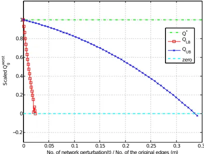
Fig. 3. A simple network (6 nodes, 7 edges): The true worst modularity indicated by the black circled line is tightly confined by the upper and the lower bounds.
A. A simple network
The network shown in Fig. 2 has six nodes and seven edges. The two modules, red and blue, are the optimal partition. The upper and lower robustness bounds are illustrated in Fig. 3. The true worst perturbation found by an exhaustive search is indicated in the black circled line. The upper bound presents the worst case perturbation scenario and t = 0
corresponds to the original network without any perturbation. The first negative value corresponds to the smallest number of perturbations that make the original two module partition invalid. The perturbed network in Fig. 2 shows the worst case perturbation. After removing the three edges, one module disappears and this leaves only the blue module with an additional node that originally belongs to the red module. The lower bound shows that the modularity measure will be negative for the three perturbations. Note that the negative modularity implies that the original partition is destroyed. The robustness of the network module is measured as 43% (addition/removal of three edges out of seven edges) where the upper and lower bounds become negative at the same level of perturbations, i.e.,t= 3.
B. Karate network
The robustness analysis result of the Karate network is shown in Fig. 4. This Karate network illustrates the actual social division that took place among people in a Karate Club in America in 1970’s where each node represents an individual member and each edge denotes the relationship between two members in the club [7]. From the robustness analysis of this division, we found that such division can hold up to 16% perturbations (t/m) before the lower bound becomes negative. An exhaustive search is not possible for this network since there are too many combinations. The minimum worst change (t/m) found in order to resolve the social division is 42%¯ perturbation. This implies that if a perturbation corresponding to this upper bound is applied so that some relations are prohibited and new connections are encouraged, the social division might be resolved.
0 0.05 0.1 0.15 0.2 0.25 0.3 0.35 0.4 0.45 −0.2
0 0.2 0.4 0.6 0.8 1
No. of network perturbation(t) / No. of the original edges (m)
S
ca
le
d
Qg
w
or
st
Q* QLB QUB
zero
[image:6.612.333.537.264.418.2]t / m t / m
Fig. 4. Karate network (34 nodes, 78 edges): The worst upper bound (¯t/m) indicates that minimum 42% perturbations in the edges can destroy the modularity. The worst lower bound (t/m) shows that the modularity will become negative by 16% perturbations.
0 0.05 0.1 0.15 0.2 0.25 0.3 0.35 −0.2
0 0.2 0.4 0.6 0.8 1
No. of network perturbation(t) / No. of the original edges (m)
S
ca
le
d
Qg
w
or
st
Q* QLB QUB
zero
Fig. 5. Yeast PPI network (1004 nodes, 8319 edges): Addition and/or removal of 34% edges (¯t/m) will void any modularity of this network. The worst lower bound (t/m) indicates that the modularity will become negative by 2% perturbations
C. Yeast protein-protein interaction network
The protein-protein interaction (PPI) network of yeast is a well-characterized biological interaction network [15]. Each node in this network represents a particular protein and each edge connecting two proteins indicates an identified biomolec-ular interaction between them. The network has several iso-lated groups and the largest one composed of 1,004 nodes and 8,319 edges and is used in this analysis. The worst lower bound shown in Fig. 5 is 2% and this indicates that we might have a very conservative lower bound, which is not close to the worst upper bound, 34% perturbation. It might be the opposite case where the upper bound is conservative and the lower bound indeed indicates the extreme fragility of the network modularity structure. This is an unavoidable result in any bounding algorithms corresponding to an NP-hard problem.
D. Citation Network
300 350 400 450 500 550 600 650 700 10−4
10−3 10−2 10−1 100
time [days]
No.
of
perturbatio
ns
(t)
/
No.
of
notes
(m)
Citation Network Citation Network Scale−Free Network
Scale−Free Network
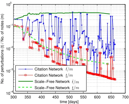
Fig. 6. Comparison of the upper and lower bound perturbations between the citation network and the scale-free network
arxiv (http://arxiv.org) [16]. The information about how each paper cited others is available as a network growth data set. In this network, two papers are connected by an edge if one of them cites the other. A complete history of citations of all papers in the database is available from the beginning date of the website. In the first year, the size of the network is very small and the number of papers reached around 20 at the 304th day. The number of nodes grows up to 2500 per year since the 304th day. In order to compare the characteristics of the citation network, the time history of an artificial network data is constructed using one of the well-known scale-free network generating algorithms, the preferential attachment [17].
The modularity robustness analysis is performed as follows: i) current network is divided into two modules, ii) the worst upper (¯t/m) and lower (t/m) bounds are calculated using the bounds algorithms, iii) once additional nodes with connections to the existing nodes are introduced, the additional nodes are distributed optimally to the existing two modules by maximising the modularity,Q, iv) if the modularity is negative, then we go to step i), otherwise we go to step ii) with the updated network by the additional nodes and edges. In other words, the worst bounds for the current module are calculated until the module is broken down. Once it is broken down, then a new modular structure is found and repeat the calculation.
The number of increasing nodes is roughly the same for both networks. Fig. 6 shows the worst bounds histories for both networks. The gap between the bounds for the scale-free network becomes larger as time evolves and the initial modular structure remains the same. The increasing gap with time is mainly caused by the conservatism of the lower bound calculation. On the other hand, the lower bound for the citation network is not conservative and the gap between them is very small once in a while, which implies there is a highly dynamic mixing nature of the citation modularity. The citation modules are not fixed but there exists a strong mixing and re-organising force in the network, which seems quite normal in an academic society with some narrow concentrated topics. This is completely opposite to the modularity dynamics of the scale-free network since the scale-free network always
maintains the original modular structure. In other networks, these mixing forces and the modularity conservation energy might be balanced in some ways.
IV. CONCLUSIONS& FUTUREWORKS
An efficient algorithm for the robustness analysis of network modularity is developed. The algorithm calculates the lower and upper bounds of robustness with respect to structural perturbation of the network. The computational cost does not increase exponentially with the number of nodes. Hence, the bounds for a time-varying network, i.e., nodes alterations, can be obtained by applying the algorithm for each fixed time without incurring a significant computational cost.
The tightness of the bounds is case dependent. Some optimization algorithms can be further employed to obtain a tighter bound with the cost of increasing computational time. In general, however, the modular structure starts breaking down from the submodules, which have a smaller number of nodes. In most cases we are more interested in the robustness analysis of small to medium size networks. Therefore, the proposed algorithms can provide valuable information on the fundamental robustness nature of modular structures of complex networks in many practical cases.
The bound estimation algorithms assume that a modular partition, which might not be optimal, is provided based on the modularity definition. As long as the partition is not significantly different from the true, it is unlikely that the worst perturbation would enhance the true partition. However, there are several degeneracy cases for finding the commu-nity structures by maximizing the modularity as shown in [18]. Whenever the robustness analysis shows that a network module is fragile, then the modularity partition should be re-investigated whether there exists a better partition.
As one of the important future works, network perturbations corresponding to minimizing or maximising the modularity could be identified as malicious attacks to the network or defence mechanisms of the network. This leads to a min-max optimization problem and it would be one of the ways to design robust network structure with respect to external disturbances.
ACKNOWLEDGEMENT
[image:7.612.63.286.50.229.2]APPENDIX
DERIVATION OF(2) ExpandQg as follows:
Minimize
∆A
Qg(s∗,∆A)
= 1 1 +α
Q∗
+ 1 4m
s∗T∆
11s∗− 1
2m(1 +α)
×2s∗TkδT ks
∗
+s∗Tδ kδTks
∗
−αs∗TkkTs∗io
.
For a fixed α, the minimisation problem is reduced to
Minimize
∆11∈D q(∆11) := s∗T∆
11s∗
−2m(1 +1 α)2s∗TkδT ks
∗
+s∗Tδ kδTks
∗
.
Re-arrange
∆11s∗=
dT 1 dT 2 .. . dT n s∗ =
s∗Td
1 s∗Td
2 .. . s∗Td
n
= In⊗s∗T d1 d2 .. . dn ,
wheredT
i is thei-th row of∆11,In isn×nidentity matrix,
and⊗is the Kronecker product. As∆11is a symmetric matrix andn2 elements of d
i for i= 1,2, . . . , nare not completely
independent but only n(n−1)/2 elements are independent. By defining a matrix L appropriately, the following can be found: d1 d2 .. . dn :=L
d21..n d32..n .. . d(n−1)..n
n−2 dn..n
n−1
=Ld˜v,
where dj..n
i is the vector only taking the elements from
j-th to n-th elements of di for i = 1,2, . . . , n−1 and j =
2,3, . . . , n−1.
In addition, each element of d˜v cannot be freely +1 (add edges) or -1 (remove edges) but it can be only +1 or -1 if the corresponding element of Ais 0 (no edge) or 1 (pre-existing edge). In order to restrict each element ofd˜v to 0 (no change) or 1 (change: remove the edge if there is an edge or add an edge if there is no edge) without considering the corresponding element value of A, define a diagonal matrix, Av, composed
from the element ofA, i.e.,aij,
Av:=diag[f(a12), f(a13), . . . , f(a1n),
f(a23), f(a24), . . . , .f(a2n),
. . . , f(a(n−2)(n−1)), f(a(n−2)n), f(a(n−1)n)
,
wheref(aij)is equal to -1 foraij = 1or 1 for aij = 0, for
i= 1,2, . . . , n−1andj= 2,3, . . . , n. Then,
d1 d2 .. . dn
[image:8.612.337.542.51.188.2]=Ld˜v:=LAvdv,
Fig. 7. Worst perturbation: two topological cases
wheredvis the element ofDvandDvis the set ofn(n−1)/2
dimensional vectors, whose element is either 0 or 1. Hence,
∆11s∗= In⊗s∗T
LAvdv
and
δk= ∆111= In⊗1T
LAvdv.
Finally, the minimization problem is reposed as follows:
Minimize
dv∈Dv q(
dv) =aTdv−dT
vBdv, (5)
where
a:=
"
s∗T I
n⊗s∗TL−
s∗Tks∗T I
n⊗1TL
m(1 +α)
#
Av,
B:= A
T
vLT In⊗1T
Ts∗s∗T I n⊗1T
LAv
2m(1 +α) .
AsB is a rank one matrix,
Minimize
dv∈Dv q(
dv) =aTdv−dT
vbeTdv,
where B = beT, each element in b is the magnitude of
each row vector of B and e is the unit vector spanning the one-dimensional row space of B. Note that B is symmetric andbandeare parallel. Hence, (2) is obtained.
INEQUALITY FORθ1
Proposition A.1: θ1andθ2are related to each other asθ2=
π+θ−θ1for θ+θ1+θ2> πor θ2=π−θ−θ1 otherwise, where θ is the angle between a and −b. θ1 is in the range betweenθ1 andθ1, where¯
θ1:= min(θ1) = cos
−1
P i∈M¯ ai
a√t
,
which is greater than or equal to zero, M¯ is the index set whose elements are the indices of the firstt-number of largest elements ina,
¯
θ1:= max(θ1) = cos−1
P i∈Mai
a√t
!
,
elements in a.
Proof: As shown in Fig. 7, without loss of generality dv is assumed to be in the plane formed by a and b as the perpendicular component of dv to the plane does not have any effect on the value of q(dv). There are two geometrical cases for θ2, i.e., θ2 =π+θ−θ1 for θ+θ1+θ2 > π or θ2=π−θ−θ1 otherwise. By the definition, θ1is given by
θ1= cos−1
aTd v
a√t
,
and cos(θ1) is a monotonically decreasing function for θ1∈[0, π]. Hence, for a fixedt, i.e., the number of 1’s indv, the minimum or the maximum of θ1occurs at the summation of the maximum or the minimumt-number of elements ina.
QUARTIC EQUATION
Proposition A.2: q(dv)in (3) is equivalent to
Minimize
θ1∈[θ
1,θ¯1]
q(θ1) =a√tx−bt(xcosθ±p1−x2sinθ)2, where x= cosθ1, and the following inequality is satisfied if θ1 takes any values between θ1 andθ1:¯
minq(θ1)≤minq(dv).
Proof: The magnitude ofdv is √t and (3) becomes
q(dv) =a√tcosθ1−btcos2θ2. Substituteθ2=π±θ−θ1 into the above
q(θ1) =a√tcosθ1−btcos2(±θ−θ1)
=a√tcosθ1−bt(cosθcosθ1±sinθsinθ1)2, and sinθ1 =√1−cos2θ1 for θ1∈[θ
1,θ1¯ ].θ1 is allowed to be any angle between θ1 andθ1. However, not all angles in¯
[θ1,θ1¯] are feasible by dv as its elements are restricted into
either 0 or 1. Hence, minq(θ1) is always less than or equal tominq(dv).
Proposition A.3: Let q(θ∗
1) = minq(θ1) and θ1∗ is equal to θ1, θ1¯ or cos
−1x∗
, where x∗
is the solution of quartic polynomial equation:P4
i=0wixi = 0, whose coefficients are
given by the following two cases:
w4= 4b2t2h4 sin2θcos2θ+ 2 cos2θ−12i
,
w3=−4abt√t 2 cos2θ−1
,
w2=−16b2t2sin2θcos2θ+a2t2−4b2t2 2 cos2θ−12
, w1= 4abt√t 2 cos2θ−1
, w0= 4b2t2sin2θcos2θ−a2t, or
w4= 4b2t2 2 cos2θ−12
, w3=−4abt√t 2 cos2θ−1
,
w2=a2t2−4b2t2 2 cos2θ−12
, w1= 4abt√t 2 cos2θ−1
, w0= 4b2t2sin2θcos2θ−a2t,
andx∈[−1,1]. Proof: θ∗
1 will occur either on the boundary, i.e.,θ1 orθ1, or¯ the angles in(θ1,θ1¯ ), where the derivative ofq(θ1)is equal to zero.
dq(θ∗
1) dθ1 =
dq(θ∗
1) dx
dx dθ∗
1
=−dq(θ ∗
1) dx sinθ
∗
1 = 0. Immediate solutions fromsinθ∗
1= 0areθ
∗
1 = 0orπand they would be either on the boundary of the domain ofθ1or outside of the boundary. Hence, they are automatically considered when the boundary values are checked. The remaining θ∗
1 values to be checked are the ones making the derivative equal to zero. Take the derivative
dq(θ)
dx =a
√
t−2bt 2 cos2θ−1
x
∓2btsinθcosθp1−x2±2btsinθcosθ x 2
√
1−x2 = 0. After squaring both sides and some algebraic manipulations, which is tedious and omitted, it leads to the two quartic polynomials inx.
INEQUALITY FOR THE UPPER BOUND
Proposition A.4: The minimum ofq(dv)is bounded above by
min
dv∈Dvq(
dv)≤q(¯dv), where
q(¯dv) =
¯
αaT1Avd¯v+p(¯dv)
×(1 + ¯α)−1, p(dv) := aT1 −a˜T2
Avdv−dTvb˜b˜Tdv,
aT1 :=s∗T I
n⊗s∗TL,
˜
aT2 :=s∗Tks∗T I
n⊗1TL×m−1,
˜
b:=ATvLT In⊗1TTs∗
×(√2m)−1,
¯
dv:= argmin dv∈Dv
p(dv),
¯
α:=1TAvd¯v.
Proof) Recall (5) in Appendix and rearrange it as follows:
Minimize
dv∈Dv q( dv) =
aT1 − ˜a
T
2
(1 +α)
Avdv−dTv
˜
bb˜T
(1 +α)dv = 1
1 +α
n
(1 +α)aT1 −˜aT2
Avdv−dTvb˜b˜Tdv o
.
minp(dv) is the minimizing solution of only parts of q(dv) and the corresponding solution, (¯dv,α¯), is substituted into q(dv), which is equal toq(¯dv). Hence,minq(dv)≤q(¯dv).
Proposition A.5: The following inequality is satisfied:
q(¯dv)≤q(˜dv), where
˜
i.e., T(·) is the operator to transform dˆv in Dvv to the
correspondingdvinDv. For example, forl= 3,d˜v= [1 0 0], thend˜v=T(ˆdv) =T([1 0 0]) = [1 1 0]T.
Proof) As d˜v is transformed from the minimizing solution of pˆ(ˆdv) by T(·). By the definitions, p(˜dv) is greater than or equal to minp(dv). Hence, q(˜dv) is also greater than or equal to q(¯dv).
PROOF OFTHEOREM2.3
As each submodule is part of a whole network, the modu-larity definition for a submodule is as follows [2]:
Maximize
s∈S Q(
s, Asg) = 1
4ms
TBsgs,
where
Bsg=Asg−21mksgksgT −diagh˜ksg1 , ˜ksg2 , . . . , ˜ksgn
g
i
+ 1 2mdiag
k1sg1Tksg, k
sg
2 1Tksg, . . . , knsgg1
Tksg
,
Bsg is scaled by the last two terms in order to evaluate the
modularity in the whole network,Asg is the adjacency matrix
including only the concerned submodule,
˜
kisg= ng
X
j=1 Asgij,
for i= 1,2, . . . , ng,
ksg=Pn j=1Al1j,
Pn
j=1Al2j, . . . ,
Pn j=1Alngj
T
,
l1, l2, . . . , lng are the indices including the nodes that
be-long to the submodule, and ng is the number of nodes in the
submodule. Re-arrange Qfor submodule
Q(s, Asg) =sT 1
4m
Asg− 1
2mk
sgksgT
s
−41msT
s1˜k1sg s2˜k2sg . . . sng˜k
sg ng + 1 8m2s
Tdiag
ksg1 1Tksg
ksg2 1Tksg
.. . ksg
ng1
Tksg s
=sT 1
4m
Asg−21mksgksgT
s−s
Tdiag[s]
4m k˜
sg
+ksgTdiag[s] s1
T
8m2 k
sg,
wherek˜sg is the vector constructed by ˜ksg
i . Note that
pertur-bations only occur in the submodule, i.e. Asg
g =Asg+ ∆11,
hence
ksg
g =ksg+δk andk˜sgg = ˜ksg+δk.
Then,
Q(∆11) =s∗T 1
4mg
Asgg −
1 2mg
ksgg ksgTg
s∗
−s
∗Tdiag[s∗
] 4mg
˜
ksg
g +ksgTg
diag[s∗
] s∗
1T
8m2
g
ksg
g ,
wheres∗= argmaxQ(s, Asg). The worst-case analysis
prob-lem is given by
Minimize
∆11∈Dsg Q(∆11) = s∗T 1
4mg
Asg g −
1 2mg
ksgg ksgTg
s∗
−s
∗Tdiag[s∗
] 4mg
˜
ksg
g +ksgTg
diag[s∗
] s∗
1T
8m2
g
ksg
g ,
where the first term in the right hand side has exactly the same form as the one in the whole network andmg can be written
as
2mg=1TAg1=1TA1+1T∆111= 2m(1 +αsg), andαsg =δsg
m/m. From the same logic as before, there are
two extreme perturbations and
−m˜ sg
m ≤α
sg ≤ nsg(nsg−1)
2m −
˜
msg
m .
With two additional terms in the right hand side, the worst sub-modularity is
Qsg g
worst
(αsg) = 1
1 +αsg "
Q∗
+α
sg(ksg·s∗)2
8m2(1 +αsg) +
qsg∗
4m
#
,
and the robustness analysis sub-problem is given by
Minimize
dv∈Dsgv q
sg(d v) = "
s∗T I ng ⊗s
∗T
Lsg−s
∗Tksgs∗T I
ng⊗1TLsg
m(1 +αsg)
#
Asgv dv
−dTv A
sgT
v LsgT Ing⊗1
TT
s∗s∗T I ng⊗1
T
LsgAsg v
2m(1 +αsg) dv −s∗Tdiag[s∗
]δk+ksgT
g
diag[s∗] s∗
1T
2m(1 +αsg) k sg g ,
whereαsg,Lsg andAsg
v are defined similarly toα,LandAv,
respectively. The last two terms in the right hand side become
s∗T
diag[s∗
]δk=1Tδk= 2δsg
m = 2αsgm,
and
ksgTg diag[s
∗] s∗
1T
2m(1 +αsg) k sg g =
ksgT+δT k
1(ksg+δ
k)
2m(1 +αsg)
=
ksgT +δT k
(2msg+ 2δsg m)1
2m(1 +αsg) =
2 (msg+αsgm)2 m(1 +αsg) ,
wheremsg =1Tksg/2 andδsg
m =1Tδk/2.
REFERENCES
[1] E. Ravasz, A. L. Somera, D. A. Mongru, Z. N. Oltvai, and A. L. Barab´asi, “Hierarchical organization of modularity in metabolic networks.” Science (New York, N.Y.), vol. 297, no. 5586, pp. 1551– 1555, Aug. 2002. [Online]. Available: http://dx.doi.org/10.1126/science. 1073374
[3] F. Radicchi, C. Castellano, F. Cecconi, V. Loreto, and D. Parisi, “Defining and identifying communities in networks,” Proceedings of the National Academy of Sciences of the United States of America, vol. 101, no. 9, pp. 2658–2663, Mar. 2004. [Online]. Available: http://dx.doi.org/10.1073/pnas.0400054101
[4] M. E. J. Newman and M. Girvan, “Finding and evaluating community structure in networks,”Physical Review E, vol. 69, no. 2, pp. 026 113+, Aug. 2003. [Online]. Available: http://dx.doi.org/10.1103/physreve.69. 026113
[5] Y.-Y. Ahn, J. P. Bagrow, and S. Lehmann, “Link communities reveal multiscale complexity in networks,” Nature, vol. 466, no. 7307, pp. 761–764, Aug. 2010. [Online]. Available: http://dx.doi.org/10.1038/ nature09182
[6] I.-C. Morarescu and A. Girard, “Opinion dynamics with decaying confidence: Application to community detection in graphs,”Automatic Control, IEEE Transactions on, vol. 56, no. 8, pp. 1862–1873, 2011. [7] W. W. Zachary, “An Information Flow Model for Conflict and Fission in
Small Groups,”Journal of Anthropological Research, vol. 33, no. 4, pp. 452–473, 1977. [Online]. Available: http://dx.doi.org/10.2307/3629752 [8] H. Kitano, “Biological robustness,” Nat Rev Genet, vol. 5, no. 11,
pp. 826–837, Nov. 2004. [Online]. Available: http://dx.doi.org/10.1038/ nrg1471
[9] J. C. Doyle, D. L. Alderson, L. Li, S. Low, M. Roughan, S. Shalunov, R. Tanaka, and W. Willinger, “The robust yet fragile nature of the Internet,” Proceedings of the National Academy of Sciences of the United States of America, vol. 102, no. 41, pp. 14 497–14 502, Oct. 2005. [Online]. Available: http://dx.doi.org/10.1073/pnas.0501426102 [10] N. Monshizadeh, H. Trentelman, and M. Camlibel, “Projection-based
model reduction of multi-agent systems using graph partitions,”Control of Network Systems, IEEE Transactions on, vol. 1, no. 2, pp. 145–154, June 2014.
[11] J.-D. J. Han, N. Bertin, T. Hao, D. S. Goldberg, G. F. Berriz, L. V. Zhang, D. Dupuy, A. J. M. Walhout, M. E. Cusick, F. P. Roth, and M. Vidal, “Evidence for dynamically organized modularity in the yeast protein-protein interaction network,” Nature, vol. 430, no. 6995, pp. 88–93, Jul. 2004. [Online]. Available: http://dx.doi.org/10.1038/nature02555
[12] R. Krishnadas, J. Kim, J. McLean, D. G. Batty, J. McLean, K. Millar, C. Packard, and J. Cavanagh, “The envirome and the connectome: exploring the structural noise in the human brain associated with socioeconomic deprivation,” Frontiers in Human Neuroscience, vol. 7, pp. 722+, Nov. 2013. [Online]. Available: http://dx.doi.org/10.3389/fnhum.2013.00722
[13] N. N. Batada, T. Reguly, A. Breitkreutz, L. Boucher, B.-J. Breitkreutz, L. D. Hurst, and M. Tyers, “Still Stratus Not Altocumulus: Further Evidence against the Date/Party Hub Distinction,” PLoS Biology, vol. 5, no. 6, pp. e154+, Jun. 2007. [Online]. Available: http://dx.doi.org/10.1371/journal.pbio.0050154
[14] M. P. H. Stumpf, C. Wiuf, and R. M. May, “Subnets of scale-free networks are not scale-scale-free: Sampling properties of networks,”
Proceedings of the National Academy of Sciences of the United States of America, vol. 102, no. 12, pp. 4221–4224, Mar. 2005. [Online]. Available: http://dx.doi.org/10.1073/pnas.0501179102
[15] S. R. Collins, P. Kemmeren, X.-C. Zhao, J. F. Greenblatt, F. Spencer, F. C. P. Holstege, J. S. Weissman, and N. J. Krogan, “Toward a Comprehensive Atlas of the Physical Interactome of Saccharomyces cerevisiae,” Molecular & Cellular Proteomics, vol. 6, no. 3, pp. 439–450, Mar. 2007. [Online]. Available: http://dx.doi.org/10.1074/ mcp.m600381-mcp200
[16] J. Leskovec, J. Kleinberg, and C. Faloutsos, “Graphs over time: densification laws, shrinking diameters and possible explanations,” in
Proceedings of the eleventh ACM SIGKDD international conference on Knowledge discovery in data mining, ser. KDD ’05. New York, NY, USA: ACM, 2005, pp. 177–187. [Online]. Available: http://dx.doi.org/10.1145/1081870.1081893
[17] A. Barabsi and R. Albert, “Emergence of scaling in random networks,”
Science, vol. 286, no. 5439, pp. 509–512, Oct. 1999. [Online]. Available: http://www.sciencemag.org/cgi/content/abstract/286/5439/509
[18] B. H. Good, Y.-A. de Montjoye, and A. Clauset, “The performance of modularity maximization in practical contexts,” Physical Review E, vol. 81, no. 4, pp. 046 106+, Apr. 2010. [Online]. Available: http://dx.doi.org/10.1103/physreve.81.046106
Jongrae Kim is an Associate Professor in Insti-tute of Design, Robotics & Optimisation (iDRO) and Aerospace Systems Engineering in the School of Mechanical Engineering at University of Leeds, Leeds, UK. He received the Ph.D. degree in Aerospace Engineering from Texas A&M Univer-sity, College Station, TX, USA. He was a Post-Doctoral Researcher with the University of Califor-nia, Santa Barbara, CA, USA, in 2002 and 2003 and a Research Associate with the University of Leicester, Leicester, U.K., in 2004 and 2007. He was a Lecturer in Biomedical Engineering/Aerospace Sciences, University of Glasgow, Glasgow, U.K., in 2007 and 2014. His main research interests are in the area of robustness analysis, optimal control and estimation, large-scale network analysis, system identification, dynamics, robotics, molecular biology, and neuroscience (http://robustlab.org).