Computational Complexity of Electrical Power System Problems

(1)

Computational Complexity of

Electrical Power System Problems

Karsten Lehmann

A thesis submitted for the degree of

Doctor of Philosophy

The Australian National University

(2)

(3)

Except where otherwise indicated, this thesis is my own original work.

(4)

(5)

Acknowledgments

Foremost, I would like to thank my primary supervisor Alban Grastien. His door was always open for me (figuratively, his office does not have a door), whether for discussions about work or the latest board game we played. I am very grateful to have had such a smart and supportive supervisor. I also want to express my thanks to my panel chair Sylvie Thiébaux. Her support and guidance, in times when I was struggling, were essential to allow me to make progress on this journey. I want to thank my secondary supervisor, Pascal van Hentenryck, for trying to make me see the big picture.

A big thanks goes to my colleague, Paul Scott, for all the insightful discussions about our work and for his patience with me and my questions about the English language. I am also very grateful to Carlton Coffrin for his scientific advice and for sharing his knowledge and passion ; and to Hassan Hijazi for all the help and fruitful discussions about my work.

Last but not least, I particularly want to thank my partner Christina Burt for invit-ing me to Melbourne and into her heart. I cannot imagine I would have gotten this far without her support, patience, corrections and advice.

(6)

(7)

Abstract

The study of the computational complexity of real-world applications, although the-oretical, can provide many pragmatic outcomes. For example, demonstrating that some types of algorithms cannot exist to solve the problem; the creation of challeng-ing benchmark examples; and new insights into the underlchalleng-ing structure and proper-ties of the problem. In this thesis, we study the computational complexity of several important problems in the application of electrical power systems.

Knowledge of the current state of the power system is important for power net-work operators. This helps, for example, to predict if the netnet-work is trending towards an undesirable state of operation, or if a power line is working at its operational limits. The state of a power system is determined by the demand, the generation and the bus voltage magnitudes and phase angles. The demand of loads can be reliably estimated via forecasts, historic records and/or measurements and the operators of generators report the generation values. Given generation and demand values, the voltage mag-nitudes and phase angles can be computed. This is what is called the POWER FLOW (PF) problem. Cost for generating power often varies from generator to generator. In the OPTIMALPOWERFLOW(OPF) problem, the aim is to find the cheapest generation dispatch, such that the forecast demand can be satisfied. Disasters, such as storms or floods, and operator errors have to potential to destroy parts of the network. This can make it impossible to satisfy all the demand. In the MAXIMUM POWERFLOW(MPF) problem, the aim is to find a generation dispatch that can satisfy as much demand as possible.

In this thesis, we provide the proofs that the MPF, OPF and the PF problem are NP-hard for: radial networks in the Alternating Current (AC) power flow model and planar networks in the Linear AC Approximation (DC) power flow model with line switching. Furthermore, we show that there does not exist a polynomial approxi-mation algorithm for the OPF problem in any of these settings. We also study the complexity of the Lossless-Sin AC Approximation (SIN) power flow model, showing that the MPF and OPF problem are stronglyNP-hard for planar networks.

(8)

(9)

List of Figures

2.1 The networkNeshowing all graphical features used in this thesis. . . . 14 3.1 The common pattern found in manySSPbased reductions. . . 22 4.1 An example of a network where switching of lines makes a difference

for the MPF and the OPF. . . 29 4.2 The phase-angle-difference choice networkAx

r,l. . . 31 4.3 The two possible solutions of a phase-angle difference choice network

Ax

r,l[G

p

r=-1|Lp_l=1]. . . 32 4.4 The reduction of anSSPinstance presented in Theorem 4.3.4. . . 33 4.5 The load-choice networkLex_e. . . 36

4.6 Two different solutions of Le x

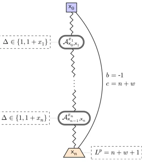
e in the case where the connector e is a generator and a load. . . 36 4.7 The networkNS,w from Theorem 4.4.4 for theSSP instance(S, w)with

S =_{x₁, . . . , x_n}. . . 38

4.8 The networkNS,w from Theorem 4.5.2 for theSSP instance(S, w)with S =_{x₁, . . . , x_n}. . . 41

4.9 Presenting the network NG from Theorem 4.5.5 for the graph G :=

({e,w₂,w₃,s},{s←→e←→w₂←→w₃←→s←→w₂}). . . 43

5.1 Thesinchoice network_Dex. . . 54 5.2 The flows along the pathe←→d(sin(2y)) and the pathe←→s←→a(sin(y))

dependent ony. . . 55

5.3 An example for the X3C instance(X, S)whereX:={x₁,x₂,x₃,x₄,x₅,x₆}

andS :=_{{x₁,x₂,x3},_{x₂,x₃,x4},_{x₃,x₄,x5},_{x₄,x₅,x6}}used in

Theo-rem 5.2.5. . . 57 5.4 An optimal solution for the example from Fig. 5.3. . . 58 5.5 From the proof of Lemma 5.2.4: a nodes ∈ S of degree two or three;

the neighbors of s in some planar layout; and the added edges which bypasss. . . 59 5.6 The networkNS,wfrom Theorem 5.3.1 for theSSPinstance({x1, . . . , xn}, w).

. . . 62 6.1 The network from Lemma 6.2.1. . . 75 6.2 The networkYex,y,v,v. . . 77 6.3 The structure of the networkMx,∆e 0,v,v,rwherez := ₁₋_cos(∆0₎1₋_r_sin(∆0₎. . 79

(12)

6.4 The ratio choice networkRs,∆,b,ge from Definition 6.3.1. . . 82 6.5 The active and reactive power flow and their ratio for a line with

sus-ceptance -1and the conductance0. . . 84 6.6 The reduction of theSSPinstance({x₁, . . . , xn}, w)used in Theorem 6.3.3.

. . . 84 6.7 The voltage choice networkVes from Definition 6.4.1. . . 86 6.8 The solution space for various active power (blue, dashed) and reactive

power (green, solid) values over the phase angle difference (y-axis) and the voltage magnitudes (x-axis). For(₋2,1), both possible solutions are

marked. . . 87 6.9 The networkNS,w from Theorem 6.4.4 for({x1, . . . , xn}, w)wherem:=

P

x∈Sxandu:=

r(1−cos(∆0_))+sin(∆0₎

1−cos(∆0₎₋_r_sin(∆0₎ . . . 90 6.10 The networkNS,wfrom Theorem 6.5.1 for({x1, . . . , xn}, w),m:=

P x∈Sx, z :=w(p0

2−p01) +mp01andy := 21

−cos(∆0_)+r_sin(∆0₎

1−cos(∆0₎₋_r_sin(∆0₎. . . 93 6.11 The setup from Lemma 6.6.1. . . 95 6.12 The solution space for various active power (dashed) values over the

phase angle difference (y-axis) and the voltage magnitudes (x-axis). . . 95 6.13 The networkT2

e using the values from Lemma 6.6.3. . . 97 6.14 The networkNS,w from Theorem 6.6.5 for({x1, . . . , xn}, w)wherem:=

P

(13)

List of Tables

1.1 Overview of all results of this thesis and including the results from Bi-enstock and Mattia [2007] (1), Kocuk et al. [2014] (2), and Verma [2009]

(2). . . 4

4.1 DC Model with Line Switching (DS Model) Result Overview . . . 26

5.1 SIN Model Result Overview . . . 52

6.1 AC Model Result Overview . . . 67

(14)

(15)

Chapter 1

Introduction

An electricalpower systemis a network of powergeneratorsandloads, typically defined

on nodes, and transmissionlinesnaturally defined on edges. Many interesting

ques-tions arise from such a network. For example, how vulnerable is the network to line disconnection, how is theflowinfluenced by the existence of specific edges, and how

can we use the knowledge of some part of the network to infer or determine the state of the other parts, specifically those parts that can change, i.e. variables.

Many interesting computational problems in electrical power systems are about determining the values of bus voltages of the system. This is called the POWERFLOW (PF) problem and was introduced by Ward and Hale [1956]. Other computational problems in power systems optimize an objective function, e.g. the optimal generation dispatch problem also called OPTIMAL POWERFLOW (OPF) introduced by Carpen-tier [1962] and the MAXIMUM POWER FLOW(MPF) as discussed by Adibi [2000]. A variety of optimization applications in power systems also involve adding or remov-ing lines in a power network. These include transmission extension plannremov-ing Hobbs [1995]; Bent et al. [2010], vulnerability analysis Alsac and Stott [1974]; Bienstock and Verma [2010], and power restoration Yolcu et al. [1983]. The switching of lines may also help to improve “optimal” solutions to the OPF and MPF problems, e.g. Fisher et al. [2008]; Van Hentenryck et al. [2011].

Researchers and engineers around the world are faced with finding algorithms to solve these power system related computational problems. The theory of computa-tional complexity enables these scientist to classify computacomputa-tional problems according to their inherent difficulty. The classes to which a problem belongs to define the types of algorithms that can solve the problem. Conversely, by showing that a problem is not included in a class, we are able to rule out the existence of the corresponding types of algorithms. For example, if a problem isNP-hard, we can rule out the existence of a polynomial time algorithm unlessP=NP. Furthermore, the instances of the problem obtained by the reduction can serve as “hard to solve” test cases.

The flow of power is given by theAlternating Current(AC) power flow equations.

These describe a non-convex solution set. Furthermore, Klos and Kerner [1975]; Klos and Wojcicka [1991] and Iba et al. [1990] showed that the PF problem can have mul-tiple solutions and Bukhsh et al. [2013] provided examples illustrating that the OPF problem can have locally optimal solutions. This is why computational problems

(16)

ing the AC power flow equations are perceived to be NP-hard1_{. The challenge to}

solve these problems sparked a lot of research, especially for the OPF problem, see e.g. Alsac et al. [1990]; Huneault et al. [1991]; Momoh et al. [1999a,b]; Baldick [2006]; Pandya and Joshi [2008]; AlRashidi and El-Hawary [2009]; Frank et al. [2012a,b] for overviews.

As solving the AC equations is challenging, current practice in the electricity in-dustry is to use the Linear AC Approximation (so-called DC model) (O’Neill et al.

[2011]). The DC model was presented by Schweppe and Rom [1970] to approximate the PF problem. It exploits the usually tight bounds for voltage magnitudes and the

small voltage phase angle differences in real life network operations. Furthermore, it

ignores reactive power. This makes the DC model linear and hence easy to solve by

design. Armed with an easy-to-solve approximation of AC power flow based prob-lems, researchers have been interested in analyzing the impact of particular complex problems, such asline switching. Line switching is the problem of changing the set of

lines in the network to achieve a particular goal, i.e. improving on optimal solutions of the OPF problem.

The first proof ofNP-hardness for the OPF and the MPF over the AC power flow model was given for a cyclic network structure by Verma [2009]. The proof was done for theLossless-SinAC Approximation(SIN), a variant of DC which uses a sine

func-tion around the voltage phase angle difference. From an AC perspective, this means that conductances are0, voltage magnitudes are all fixed at1, and reactive power is ignored2_{. The first proof of}_{NP-completeness for the OPF, MPF and the PF problem}

over the DC model with line switching (called DS model) was given for a series-parallel network structure with an unbounded maximum node degree3 _{by Kocuk}

et al. [2014]4_.

In this thesis, we present the first comprehensive study of the computational com-plexity of the OPF, MPF and the PF problem over the AC, SIN and the DS model. In particular, we improve on the results from Verma [2009] and Kocuk et al. [2014] by presenting reductions with more realistic network structures. We also investigate the complexity of approximating the OPF. We investigate the SIN model separately from the AC model as the SIN model is close to the DC model, property-wise and by appearance, yet it is a special case of the AC model. Hence, any result about the SIN model indicates that any model “in between” the AC and the DC will have similar complexity.

The detailed contributions of the thesis and its organization are as follows. We first

1_{The non-convexity of the problem does not automatically imply that problems based on the AC}

power flow areNP-hard. For example, the family of optimization problemsminysuch that0 ≤y ≤

Qn

i=1xiwheren ∈ Nhas a non-convex constraint and a non-convex solution set but the solution is

alwaysy= 0. Hence, the problem can be solved in constant time.

2_{“Ignoring” reactive power can be achieved by placing a generator with unbounded reactive power}

at every bus.

3_{The degree of a node is the number of edges/lines it has.}

(17)

3

describe the basic mathematical notations of this thesis in Chapter 2. Then, in Chap-ter 3, we present a discussion about the properties of our reductions and introduce in an abstract way, the idea on which the majority of reductions in this thesis are based.

In Chapter 4, we present the mathematical definitions and the results regarding the DC model with line switching (DS model). We show that the DS-MPF and DS-OPF for cacti5_{networks with a bounded maximum degree are}_{NP-complete. Furthermore,}

we show that the DS-OPF for cacti cannot be approximated and that the DS-PF prob-lem is NP-complete for series-parallel networks with a bounded maximum degree. All problems are easy for trees and cacti are a simple extension of trees. Hence, we can derive that any type of network structure will beNP-complete.

In Chapter 5, we present the mathematical definitions and the results regarding the SIN model. We show that the SIN-OPF and SIN-MPF are stronglyNP-hard for a planar network structure with a bounded maximum degree. We also show that the SIN-OPF cannot be approximated for a planar network structure with arbitrary maximum degree.

In Chapter 6, we present the mathematical definitions, results and a review of related work regarding the AC model. Here we show that the AC-MPF, AC-OPF and AC-PF problem areNP-hard for a tree network structure. We also show that the AC-OPF cannot be approximated.

In Table 1.1, we present an overview of all major results. The overview contains a selection of properties of our reductions: number of generators (nG), number of loads (nL), maximum bus degree (mD) and network structure (Structure). The table also includes the results from Bienstock and Mattia [2007] (1), Verma [2009] (3) and Kocuk et al. [2014] (2) as well as the results which can be easily derived from these papers. Note that Bienstock and Mattia [2007] did not present a proof. Hence, the properties of the reduction are unknown.

In Chapter 7, we draw conclusions and discuss open problems and questions.

(18)

Problem Result Structure mD nG nL Theorem DS-PF NP-complete series-parallel 3 1 1 4.3.4

DS-OPF not APX cacti 3 ∞ ∞ 4.4.4

DS-OPF NP-complete cacti 3 ∞ ∞ 4.4.5

DS-OPF NP-complete series-parallel 3 2 1 4.4.6

DS-MPF NP-complete cacti 3 ∞ ∞ 4.5.2

DS-MPF NP-complete series-parallel 3 1 1 4.5.3

DS-MPF not APX arbitrary ∞ 6 6 4.5.5

DS-MPF stronglyNP-complete planar 3 1 1 4.5.6

DS-PF NP-complete ? ? ? ? (1)

DS-PF NP-complete series-parallel ∞ 1 1 (2)

DS-OPF NP-complete series-parallel ∞ 1 1 (2)

DS-MPF NP-complete series-parallel ∞ 1 1 (2)

AC-MPF NP-hard tree ∞ ∞ 1 6.3.3

AC-PF NP-hard tree ∞ 1 ∞ 6.4.4

AC-OPF not APX tree ∞ 2 ∞ 6.5.1

AC-OPF NP-hard tree ∞ 2 ∞ 6.5.2

AC-OPF not APX tree ∞ ∞ 1 6.5.3

AC-OPF NP-hard tree ∞ ∞ 1 6.5.4

VPF NP-hard tree ∞ ∞ ∞ 6.6.5

SIN-MPF stronglyNP-hard planar 6 ∞ ∞ 5.2.5

SIN-OPF not APX planar 4 ∞ ∞ 5.3.1

SIN-OPF stronglyNP-hard planar 6 ∞ ∞ 5.3.2

SIN-OPF stronglyNP-hard arbitrary ∞ ∞ 1 (3)

[image:18.595.77.475.225.589.2]

SIN-MPF stronglyNP-hard arbitrary ∞ ∞ 1 (3)

(19)

Chapter 2

Background

In the first four sections of this chapter, we present mathematical notations and defi-nitions which are shared among all result chapters (Chapters 4 to 6). These parts are essential to understand the model specific background sections within these chapters. Note that when presenting results regarding computational complexity, we will al-ways have to define specific networks. To that end, the background sections present concepts, such as the extension of a function or the sum of two networks, and nota-tions, for example variants of networks or a function for the phase angle difference. These concepts are not found in academic literature presenting methods to solve (al-gorithms, heuristics, . . . ) the problems we study because a solving method has to work for arbitrary networks.

To present our results we use the same identifier for network types, problems and objectives. For example, an OPF networkis the specific type of network used in the

definition of the OPF. The word OPF represents the function that maps every OPF network onto the optimal value of the optimization problem which is finding the gen-eration dispatch that minimizes the gengen-eration costs. The OPFproblemis the decision

variant this: decide if the OPF of a given OPF network is less or equal than a given value.

The chapter starts with concepts about functions in Section 2.1 and graphs in Sec-tion 2.2. We than present thegeneral purpose(GP) network in Section 2.3. In Section 2.4,

we introduce the basic networks for our three problem types (MPF, OPF, PF) as spe-cial cases of GP networks. Afterwards, in Section 2.5, we introduce the graphical no-tation used in this thesis. And, finally, in Section 2.7, we provide a short introduction to approximation algorithms.

2.1 Functions

At the heart of all functions in this thesis are thereal numbersRand therational numbers Qas well as functions that map to the real and rational numbers. Anextensionof a

function is any function that has the same mapping with a potentially bigger domain. One special extension is the function that extends the domain such that every new element is mapped to the same value.

(20)

Definition 2.1.1(function extension). LetX , Y be sets andz _∈R. A functiong:Y → Rextendsa functionf :X →RifX ⊆Y and∀x ∈X :f(x) =g(x). Thezextension of

f onY is the functionf_|Yz :Y →Rdefined by

∀x∈Y :f|Yz(x) := (

f(x) ifx ∈X

z ifx _∈Y _\X .

Another concept we use is thesumof two functions. The sum of two functions is

a function that sums up all values that are shared in the domains of its summons and otherwise keeps the same values.

Definition 2.1.2(function sum). LetX , Y be sets. Thesumof the functionsf :X →R

andg:Y _→Ris the functionf +g:X∪Y →Rwith∀x∈X∪Y:

(f+g)(x) :=



  

  

f(x) +g(x) ifx ∈X ∩Y

f(x) ifx _∈X _\Y

g(x) ifx ∈Y \X .

2.2 Graph

The definition of networks is based ongraphs. Furthermore, in some of our results, we

present reductions based on graph problems. To that end, we introduce the definition of a graph as well as some graph concepts and graph structures. For a given setX, let P2(X) :={Y ⊆X | |Y|= 2}be the set of all two-element sub-sets ofX.

Definition 2.2.1(graph, nodes, degree). Agraphis a tupleG = (N , E)whereN is the

set ofnodesandE ⊆ P2(N)is the set of lines. Thedegreeof a nodeais the number of edges it belongs to, i.e. |{{a,d} | {a,d} ∈E_}|.

Cyclesare a central concept for all problems related to the switching of edges/lines

(see Chapter 4). We use the concept of simple cycles to define two graph structures

important for this thesis.

Definition 2.2.2 (walk, length, path, cycle, simple cycle). A walk is a sequence of

nodes a₁,a₂. . . ,a_n−1,an such that ∀1 ≤ i < n : {ai,ai+1} ∈ E. The length of a

walk is the number of nodes it passes through, in this casen. Apathis a walk where

|{a₁, . . . ,an}|=n. Acycleis a walk where{a₁,an} ∈E. Asimple cycleis a cycle that is

also a path.

The concept ofcomponentof a graph will be used to present results related to

re-ductions bases on graph problems.

Definition 2.2.3(connected, sub-graph, component). A graph is calledconnectedif for

every pair of nodes there exists a path between them. A sub-graphof G is a graph

(N , Ee 0) with Ne ⊆ N and E0 ⊆ E. A component of G is a sub-graph G0 which is

(21)

§2.3 GPNetwork 7

Some of the reductions presented in this thesis have the structure oftrees,cactior series parallelgraphs. The connection between these three is as follows: trees are cacti,

cacti are series parallel and series parallel graphs are planar graphs.

Definition 2.2.4(tree). A connected graph is called atreeif it does not have any cycles.

Definition 2.2.5(cactus). A graph is called acactusif every two distinct simple cycles

share at most one node.

Definition 2.2.6(series-parallel). A graph is calledseries parallelif for every two edges

{a₁,d1}and{a₂,d2}no simple cycles of the forma₁,d₁, . . . ,a₂,d₂anda₁,d₁, . . . ,d₂,a₂ exist.

2.3 GP Network

The complexity results presented in this thesis are for three different problems classes: the OPTIMALPOWERFLOW(OPF), MAXIMUMPOWERFLOW(MPF) and the POWER FLOW(PF). We investigate these three problem classes on three different power flow models:Alternating Current(AC),Lossless-SinACApproximation(SIN) andLinearAC Approximation (DC). Overall we study eight different problems1. An instance of a

specific problem is a power network, ornetworkfor short. In this thesis, we use six

different network types for our eight problems. There are only six (and not eight) because the networks/instances of the SIN and the DC model are the same within a fixed problem class.

The network type for the AC based problems can be regarded as an extension of the network for DC and SIN. Hence, in this section, we present the definition of the network for DC/SIN for all three problem classes. We call these networks MPF network, OPF network and PF network. In contrast the networks for the AC power flow model based problems are called AC-MPF network, AC-OPF network and AC-PF network. These are presented in the background section of the chapter about the AC model (Section 6.1).

The three network types MPF network, OPF network and PF network are derived from a generic network type, which is calledgeneral purpose(GP) network. The three

network types for the AC model, AC-MPF network, AC-OPF network and AC-PF network are specializations of the AC network, which itself is a generalization of the GP network.

The definition of GP networks is similar to the definition of graphs. In a GP net-work, the nodes are calledbusesand the edges are calledlines.

In the AC power flow equations and for a single line, the current (flow) across the line and the voltage difference of the two ends of this line have to be constant. This constant value is calledadmittance. Since voltage and current are complex

num-bers, the admittance is complex as well. Its real part is called conductance(denoted

(22)

is a negative rational number that is used by all types of flows in this thesis. The conductance, on the other hand, is a parameter that is only used by the AC model. Its value is usually close to0for real world transmission lines. Hence, the SIN and DC model approximate the AC model by assuming that the conductance is0. When defining and graphically presenting lines in any context other than the AC model, we will omit showing the conductance as its value does not matter.

The third parameter of a line is calledline capacity(denoted withc). Its purpose is

to limit the amount of flow along a line. For none of the results about the AC model do we need the “feature” of limiting the flow along a line. Hence, we will ignore this parameter in the context of the AC model. Note that the AC model, however, has a network wide maximum phase angle difference.

Some buses are generators and some buses are loads. These are indicated as sub-sets of the set of buses. In a network, we also allow to assign values to a subset of these generators and/or loads. These values are later interpreted as given, with fixed generation and/or demand values.

Note that real-world networks also include additional components, such as trans-formers, bus shunts, line charging or phase shifters (Stott and Alsac [2012]). Our net-work definition will not include these components because we do not need them for our reductions.

Definition 2.3.1(GP network). A GP network is a tuple(N , N_G, N_L, E , Gp_{, L}p₎_where

• N is the set ofbuses,

• N_G_⊆N is the set ofgenerators,

• N_L_⊆N is the set ofloads,

• E _{⊂ P2}(N)_×Q≤0×Q2≥0 is the set of lines with

∀({a,d}, b₁, g₁, c₁),({a,d}, b₂, g₂, c₂)∈E :b₁ =b₂, g₁ =g₂andc₁ =c₂,

• Gp_:_Np

G→Q≤0 withN p

G⊆NGis the (partial)active power generation, and

• Lp _:_Np

L→Q≥0 withN p

L⊆NLis the (partial)active power demand.

In contrast to the general literature, our generators and loads do not have upper and lower bounds. Having bounds can be regarded as a “feature” which could be used by a reduction. However, only one of our reductions need this feature to work. Therefore, we omit defining it in general.

When defining GP networks (and their derivatives MPF network, OPF network and PF network) we present functions like Gp _and _Lp _{in an implicit manner. For}

example, for the functions Gp : {r} → Q≤0 , Gp(r) := -1 and Lp : {l} → Q≤0 , Lp(l) := 12we have the two equivalent representations

N := (_{e,r,l,a,d},_{r,a},_{l,d}, E , Gp, Lp) :=_{e,r,l,a,d},_{r,a},_{l,d}, E ,hGp_r=-1

L p

l=12

(23)

§2.3 GPNetwork 9

In the case where no active power generation and load values are fixed, we write∅.

Hence, we have

N := ({e,r,l,a,d},{r,a},{l,d}, E , Gp, Lp) = ({e,r,l,a,d},{r,a},{l,d}, E ,∅)

whereGp :_{∅ →}Q≥0andLp :∅ →Q≤0.

In some cases, when defining networks, we are given a set of natural numbers,

X :=_{x₁, . . . , x_{n} ⊆ P}(N)and the network has one bus per element ofX. SoX ⊆N

whereN is the set of buses. The identifier of these buses are the numbersx_i ∈X. To

aid readability we refer to the value of the number of anx_i ∈Xwithx_iand whenever

we refer to the symbol that represents the bus we use the notationx_i.

Given a GP network we sometimes provide proofs of properties for a variant of this network. A variant could be when a bus becomes a generator and load. Another way kind of creating variants is when, for example, we fix the generation of a bus and if that bus was not a generator then we make it one. As these variants are only used temporarily we define a special syntax for them based on the original network.

Definition 2.3.2(network variant). LetN = (N , N_G, N_L, E , Gp, Lp)be a GP network and Gep :N

p

G → Q≤0 andLep : N p

L → Q≥0 be active power generation and demand

functions. We define and denote the GP network variant ofN with respect toGepand e

Lpvia

N[Gep,Lep] := (N , N_G∪N_Gp, N_L∪N_Lp, E , Gp+Gep, Lp+Lep).

Lete ∈N be a bus. The GP network variant of_N, wheree becomes a generator and a load, is defined and denoted as

N[e∈N_G/L] := (N , N_G∪ {e}, N_L∪ {e}, E , Gp, Lp).

We use the notations above in the statements of lemmas. To shorten these presen-tations we never present the functionsGep andLep directly. Instead, we use a similar

implicit definition as for the definition of networks. For example, letN be a GP net-work,Gep be a generation function withGep_r := -1andLep be a demand function with

e

Lp_l = 1. Instead ofN[Gep,Lep]we writeN[Gp_r=-1|Lp_l=1]omitting the usage and

defini-tion of the symbolsGepandLep.

In most of our reductions, we define the networks by connecting multiple net-works together. The connection of two netnet-works happens along a set of common buses. To ensure that our sum of networks is well defined, we force the condition that both networks do not share any lines.

Definition 2.3.3(sum of two networks). Let N := (N , N_G, N_L, E , Gp, Lp)andNe :=

(N ,e Ne_G,Ne_L,E ,e Gep,Lep) be two GP networks with {{a,d} | ({a,d}, b, g, c) ∈ E} ∩ {{a,d} |(_{a,d}, b, g, c) _∈Ee}=∅and we defineN_a :=N ∩Ne. ThesumofN andNe

with respect toN_ais defined as

(24)

In most cases, the set N_a will consist of only one bus (which we usually denote

with e). This bus is called the connector. Note that when building the sum of two

networks, we always explicitly state at which buses they are connected together. In the case where two networks share buses other than the connector, we assume that these buses get automatically renamed before building the sum network. From the definition above, it is also easy to see that the network sum operator is associative. Hence, we will omit using parentheses when building the sum of multiple networks. IfN_ahas only one element then we omit the set brackets as well. LetX ={x₁, . . . , xn}

be a set andNxi

e be some networks with buse. We writePe_x∈X N x

e := Nex1+e. . .+e

Nxn

e .

In order to later be able to define power flows, we need the set ofdirected lines.

Definition 2.3.4(directed lines). Let(N , N_G, N_L, E , Gp, Lp)be a GP network. The set ofdirected linesisEd:={(a,d, b, g, c)|({a,d}, b, g, c)∈E}

2.3.1 GP Solutions

Before presenting the network types for MPF, OPF and PF, we introduce notations and concepts involvingsolutions. We formulate the problem classes (and their

com-plexity problems) using solutions. A solution is an allocation of values for a given and fixed set of variables: for example, the line flows or the phase angles. Furthermore, a solution has to satisfy given constraints: for example, that all line flows are within their bounds. They also have to match the given values for active power generation and active power demand.

The allocations of variables is always given as a function mapping from the sets of buses, generators, loads or directed lines into the real numbers. The variables impor-tant for networks in this thesis are the

• (voltage)phase anglesθ:N →R,

• voltage magnitudesv:N →R>0,

• active power generationGp_:_N

G →R≤0,

• reactive power generationGq_:_N

G→R,

• active power loadLp :N_L_→R≥0,

• reactive power loadLq :N_L→R,

• active power flowp:Ed→R, and

• reactive power flowq :Ed→R.

(25)

§2.3 GPNetwork 11

In the literature, one can also find active/reactive generation and load being de-fined for all buses. This is especially common in literature about solving any of our problem classes. The models in the literature, have upper and lower generation and load bounds for every bus. Buses without generator or load are expressed by setting the corresponding upper and lower bounds to0. Contrarily, our generators and loads do not have bounds. Hence, we have to restrict the generation and load functions to the sets of generators and loads. When presenting Kirchhoff’s junction law later we will use the notation of function extension (from Section 2.1) to extend the genera-tion/load function to be0for buses which are not generators/loads.

The functions presented above are usually interpreted as vectors in the literature. The assumption is that there exists some fixed order of the set of buses and the set of lines. An element of a vector is usually indicated by an index on the symbol of the vector. This motivates our notationv_a (instead ofv(a)). The same is true for all

variables where the domain is a subset of the set of buses: θ, Gp_, _Lp_, _Lq_, _Gq_{. For}

the functionp, we writepad instead ofp((a,d, b, g, c)). Similarly forq and any other function with the domain ofEd.

We call the basis of all types of solutions for our problems in this thesis: GP so-lution. These solutions pose the constraint, that at every bus the sum of all flows,

the generation and the load balances. Not present in this definition is a power flow constraint. A power flow constraint binds the power flow (active or reactive) to the phase angles (and voltage magnitudes). It is specific for the power flow model we study. Hence, these constraints are introduced in the sections for AC, DC and SIN respectively. These sections also present specific definitions for our problems.

The line parameters susceptance (b) and conductance (g) are only used in the

power flow constraint. Hence, they do not appear in the definition of a GP solu-tion. Furthermore, all power flow constraints depend on the phase angle (θ) of the

bus. Since all the specific definitions depend on the definition of a GP solution, we include the phase angle in this definition, even though it is not used here.

Definition 2.3.5 (GP solution). Let N = (N , N_G, N_L, E , Gp, Lp) be a GP network. A GP solution for _N is a tuple (θ,Gep,Lep, p) where θ : N → _R, Gep : N_G → _R_≤₀,

e Lp _:_N

L→R≥0andp:Ed→Rsuch that

• GepextendsGp,

• LepextendsLp,

• and Kirchhoff’s junction rule for active power is satisfied,

∀a∈N :Gpa +Lpa+

X

(a,d,b,g,c)∈Ed

pad = 0

whereGp _:=_G_ep_|N

0 andLp :=Lep| N 0 .

(26)

In the definition above, we distinguished between the generation function of the network,Gp _{and the generation function given by the solution}

e

Gp_{. As for solutions,} e

Gp is always an extension ofGp we will use the same symbol for both from now on.

This will happen especially when the domain ofGpis empty. The same applies toLp.

That means for a GP network(N , N_G, N_L, E , Gp, Lp), a solution could be represented

by(θ, Gp_{, L}p_{, p}₎_{where the latter}_Gp_and_Lp_{are extensions of the former.}

In the different types of solutions for the models that we have (AC, DC and SIN), the phase angles only occur in a difference of two phase angle values. This motivates us to define a function of phase angle differences.

Definition 2.3.6 (phase angle difference). Let N be a GP network and(θ, Gp_{, L}p_{, p}₎

be a GP solution. We define the function ofphase angle differences ∆ : Ed → R via

∆(a,d, b, g, c) :=θ_a−θ_d.

2.4 Problem Specific Networks

The GP networks will be specialized into three types of networks: MPF, PF and OPF network. These three are underlying networks for all SIN related problems presented in Section 5.1 and DC related problems defined in Section 4.1. They are also the basis for the AC-MPF, AC-PF and AC-OPF networks defined in Section 6.1.

2.4.1 MPF Network

For the MPF, the goal is to find the generation and demand such that we satisfy as much demand as possible. Hence, there must be some loads and generators which do not have fixed demand or generation. There could also be generators or loads which are fixed. For example, there could be the constraint that a hospital must be supplied with power. This demand creates a minimum demand at a bus which could be modeled as having one load with a fixed demand and another load that is free.

In our model, we assume that all generators and loads are not fixed. This is be-cause we do not need fixed values to establish our results. An exception is the result showing that the MPF cannot be approximated in the DC power flow model with line switching. This result needs one load with a fixed demand. The necessary definitions for this case will be presented in the section about the DC model (Section 4.1).

In our definition of MPF networks, generators and loads are disjoint. The MPF could not be well defined otherwise, because having a generator and a load at the same bus would result in a potentially infinite value for the MPF.

Definition 2.4.1(MPF network). A GP network(N , N_G, N_L, E , Gp_{, L}p₎_{is called MPF}

networkif

• N_G_∩N_L=_∅, • dom(Gp) =∅, and

(27)

§2.5 Graphical Representation 13

2.4.2 OPF Network

The goal of the OPF is to find a generation dispatch such that a given and fixed de-mand is satisfied and the overall generation cost is minimal. Hence, an OPF network has acost functionCwhich allocates costs for every generator. Also, the demand of all

loads is given. In the definition of the OPF problem in the literature, one can usually find a lower and upper bound for the generation. By setting the lower to the upper bounds to the same value one could essentially fix the generation. Although our def-inition of GP networks does not include lower and upper bounds, it does allow for the fixing of generation values. However, in our results we do not need the feature of fixed generation. Hence, in our definition of OPF network all generators are free. We also add the constraint that generators and loads are disjoint. This is because we do not need the feature of a bus being a generator and a load at the same time.

Definition 2.4.2(OPF network). An OPFnetworkis a tuple(N, C)where • N = (N , N_G, N_L, E , Gp_{, L}p₎_{is a GP network with}

• N_G_∩N_L=_∅,

• dom(Lp_{) =}_N L,

• dom(Gp) =_∅, and

• C :N_G →Q≥0 is the cost function.

2.4.3 PF Network

In the PF problem we ask the question whether or not a solution exists. It is generally assumed that the demand and the generation of all but one generator is given. This one generator (denoted withs) is called:slack bus. The intention of the slack bus is to

ensure the existence of a solution. However, as we will show in Section 6.4, this is not guaranteed. We also add the constraint that generators and loads are disjoint. This constraint makes the reductions stronger. We do not need the “feature” of having a generator and a load at the same bus.

Definition 2.4.3(PF network). A GP network(N , N_G, N_L, E , Gp_{, L}p₎_{is called PF}

net-workif

• N_G_∩N_L=_∅,

• ∃s ∈N_G:N_G\dom(Gp) ={s}, and

(28)

r Gq _{= 1}

C = 23

l Lq2 f3; 4g

a = 1

v 2 [0:9; 1:1]

e v = 1

N1

r G

q _{= 3} C = 54

N2

l L

p _{= 5} Cfix= 12

N3

a Gq+ Lq 2 f 1; 1g

N4 e;d 2 f2; 3g

d b =-1

c = 2

b =-3 g = 4

[image:28.595.105.460.95.492.2]

b =-2 c = 1 p = 5 N5

Figure 2.1: The networkNeshowing all graphical features used in this thesis.

2.5 Graphical Representation

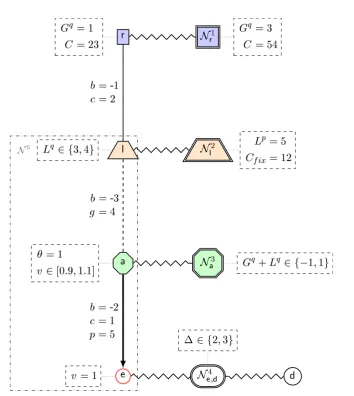
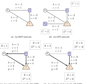
Fig. 2.1 presents all graphical features used in this thesis through the network Ne. We deviate from the classical graphical presentation of power system networks. The representation is more similar to the way graphs with their nodes and edges are pre-sented. All graphical features presented are valid for all types of models and net-works.

(29)

§2.5 Graphical Representation 15

which are part of a presented solution2_{. Note that the network}_N

e is not of any type of networks we defined earlier. Its purpose is only to present an overview of the graphical features.

Figure 2.1 tells us the following things:

• Bus r is a generator (blue rectangle) with a fixed active power generation of Gpr = 1 and (active power) cost ofCr = 23. Other variables not specified (e.g. voltage magnitude) are free.

• Buslis aload(orange trapeze) with a reactive power demand of either3or4. • Busa is agenerator and a load(green chamfered) with a fixed phase angle of

θ_a = 1and a voltage magnitude that can range from0.9to1.1.

• Buse isneither a generator nor a load(white ellipse) has a fixed voltage

mag-nitude of1.

• Busdisneither a generator nor a loadand has no fixed values.

• The busesl, a ande together with their lines form thesub-network

(dashed-dotted box)N5_.

• The liner←−→b=-1

c=2 lhas a susceptance of -1and a capacity of2. The conductance is

not shown, as this line is used in the representation of networks in the chapter about the DC model. The DC model does not use conductance.

• The line l←−→b=-3

g=4 a has a susceptance of -3 and a conductance of 4. The third

parameter for this line is not shown as the line is used in the representation of networks in the chapter about the AC model. The AC model does not use any line based capacity or phase angle restriction like the DC or the SIN model. • The linel←→aisswitched off(dashed).

• The linea←−→b=-2

c=1 e has a susceptance of -2and a capacity of1. The conductance

is not shown as this line is used in the representation of networks in the chapter about the SIN model. The SIN model does not use conductance.

• The linea←→ealso has an activepower flowofpae = 5fromatoe (indicated by the arrow direction).

• ThenetworksNr1,Nl2,Na3andNed4 are part of this network but their appearance is hidden (double shaped frame). They haveconnector buses(r,l,a,e,d) which

are the same as the ones of networkNe (indicated by the zigzag edge). Within the symbol of a network the connector bus is presented as under-script.

• The networkNepictured in Fig. 2.1has the connectore(red border color).

(30)

• The network Nr1 with connectorr acts as generator to r (blue rectangle) and generates a fixed amount of3reactive power. This implies that there is a total implicit reactive power of 4atr. Also the network generates active power for cost of54per unit.

• The networkNl2 has the connectorl and acts as loadforl with a fixed active power load of5. The value for reactive power is a free variable. Furthermore, the network hasfixed costsof12. “Fixed” means that this value does not depend

on the amount of reactive power demand taken in by the network.

• The networkNa3 acts as either generator or load(green chamfered rectangle) fora where we have thechoicebetween either generation of consuming1unit of reactive power.

• The networkN4

e,dhastwo connectorseanddwhose phase angle difference can only be either2or3.

2.6 Strongly NP-Completeness

We present a short introduction to strongly NP-completeness. More details can be

found in Garey and Johnson [1978]. StronglyNP-complete problems are a special case of NP-complete problems. A problem is calledstrongly NP-hard if the variant of it

where all numerical parameters are bounded by a single polynomial in the size of the input isNP-hard. A problem is called strongly NP-completeif it is stronglyNP-hard

and inNP. For example, the problem of finding the longest path in a graph does not have any numerical parameters and hence is stronglyNP-complete. The SUBSETSUM PROBLEM, which is widely used in this thesis, is an example of a problem which is NP-complete but not stronglyNP-hard.

A way to prove that a problem is stronglyNP-hard is to find a polynomial-time re-duction of another stronglyNP-complete problem such that all numerical parameters of the reduction are bounded by a single polynomial in the size of the input. Such a reduction is calledpseudo-polynomial reduction.

2.7 Approximation Algorithms

We present a short introduction to approximation algorithms. More details are pre-sented by Vazirani [2013]. An approximation algorithm is an algorithm designed to find a solution of an optimization problem, guaranteeing that the objective value is “not too far” from the optimal value. We are only interested in approximation algo-rithms which run in polynomial time with respect to the input size. Such algoalgo-rithms are classified by what guarantees they can provide.

LetW be set of all instances of some minimization problem; and, for an instance w ∈W, letOP T(w)be the optimal value. Furthermore, letA:W →Rbe an

(31)

§2.7 Approximation Algorithms 17

instancew. The algorithmAis called-approximationalgorithm with >1if it runs in polynomial time with respect to the input size; and it can guarantee that the objective value for each instance is not worse thantimes the optimal value. That is, if:

∀w_∈W :OP T(w)_≤A(w)_≤OP T(w).

Similarly, for maximization problems we have0< <1and

∀w∈W :OP T(w)≥A(w)≥OP T(w).

We say that an optimization problem can be approximated by aconstant factor approxi-mationif there exists at least one-approximation algorithm for some. The class of all

problems which have a constant factor approximation is calledAPX(an abbreviation

for approximable). We say an optimization problem cannot beapproximated within any constant factorif there does not exist any-approximation algorithm.

The class APX contains the problems which admit a Fully Polynomial-Time Ap-proximation Scheme(FPTAS). These are optimization problems where there exists an

-approximation with a runtime polynomial in the input and 1_/ for every . It

(32)

(33)

Chapter 3

Methods

This chapter is about aspects of computational complexity in power systems. We do not present any results here. Also, it is not necessary to read this chapter in order to understand the results in the following chapters. The purpose of this chapter is to provide additional information into the how and why of our reductions.

In Section 3.1 we present an analysis of the “features”1 _{of our reductions. A}

fea-ture could be, for example, that the networks in all reductions of a problem have one generator. We explain which features we focused on and why.

In Section 3.2 we provide an informal introduction into the idea behind most of our reductions. The goal of this section is to aid the understanding of these proofs. Afterwards, in Section 3.3, we give a similar introduction for non-approximability.

3.1 Reduction Features

Overall, there are three models and three classes of problems. This makes for eight different problems2_{. When investigating these problems for the case where there}

ex-ists an algorithm to solve them, one can wonder: does there exist a fundamentally better method to solve these problems? Studying the computational complexity of these problems can be one way to answer this question. For example, by showing that a problem isNP-hard, we can derive that no polynomial algorithm exists unless P = NP. This means that the fact that no efficient algorithm was found is simply because none exists and we can stop searching for it.

To prove that a problem isNP-hard we first have to choose anNP-hard problem. Then, we present areductionof this problem into the problem which we study. For

example, let theNP-hard problem be the SUBSETSUM PROBLEM(SSP) (defined in the following section) and our problem be the AC-PF problem. A reduction is a map-ping assigning eachSSPinstance a network such that the network has a solution (PF problem) if and only if theSSPinstance is solvable. Furthermore, the network must be computed in time polynomial in the size of theSSPinstance. This implies that the size of the network must be polynomial in the size of theSSPinstance.

1_{or the absence of them}

(34)

Of special interest are the properties that all of these networks share and the prop-erties they do not have. We call such a property afeatureof the reduction. For example,

if in all networks at least one generator has an upper bound for its generation we say that the reduction used the feature of “generation upper bounds”. If on the other hand in all of the networks, there is no load with an upper bound then we say that the reduction does not use the feature of load upper bounds.

If we have a reduction which, for example, uses the feature of generation upper bounds, then it still might be possible that there exists a polynomial algorithm which solves the problem we study for networks without generation upper bounds. Hence, it is desirable to investigate if a reduction exists which does not need the feature of generation upper bounds. Such a reduction is to be considered “stronger”. In a more general sense, we can say that the fewer features are used in a reduction, the “stronger” the reduction is. Note that the word “stronger” here is not a well defined term. The word is an indication that the networks used in the reduction are more likely to be contained in real world cases. Also, some features are not just simply on-off properties but they might have a hierarchy. The structure of the network is such a feature. A reduction which results in only planar networks is considered to be “stronger” then a reduction where the network structures are arbitrary. It is also possible that in order to not use one feature we have to use another one. For example, we might be able to find a reduction where we do not need generation upper bounds, but to make it work we have to use load upper bounds.

We aimed to find reductions which are as strong as possible. To that end, we iteratively improved our reductions . This iterative process also had the side-effect that the reductions themselves became shorter and more elegant over time. Therefore, a major contribution of this thesis is that we present reductions which only use very few features.

In the following, we present an outline of the features we focused on. The choice of features is motivated by the appearance and properties of real world power networks. Note that some features are only relevant for some power models or problem classes. For example, in the PF problem the demand is a given and fixed value. Hence, the feature of load upper bounds is irrelevant as it can be satisfied easily.

Network Structure The feature “network structure” distinguishes between the

fol-lowing from weakest to strongest: arbitrary structure, planar networks, cacti and trees. It is important because, in the real world, power networks cannot have an arbitrary structure. For example, transmission networks are usually (almost) pla-nar networks (Pagani and Aiello [2013]) and distribution networks are trees (Hijazi and Thiebaux [2014]). Hence, presenting a reduction which needs arbitrary structure might not say anything about real world networks.

Bus/Node Degree The degree of a bus is the number of lines connected to it. In real

(35)

§3.2 NP-Hardness Reduction 21

is minimal. At the very least, to be close to realistic networks, it is important to ensure that the maximum degree is bounded by a constant.

Ratio of Generators to Loads Real world power networks usually have few

gener-ators and a large number of loads. Hence, in order to be realistic, a reduction where the ratio of generators overs loads is small is desired.

Susceptance to Conductance Ratio (AC model only) Where possible, our

reduc-tions do not fix the susceptance and conductance values. Instead, we treat them as external parameters and only present necessary conditions for them to ensure that our proofs work. For example, in some proofs, the only condition we have is that both values cannot be zero at the same time. Having done the proof with abstract parameters has the advantage that essentially we provide reductions for all kinds of ratios (which satisfy the given conditions). Our main focus is to ensure that the range of valid ratios includes the range of realistic ratios. According to Andersson [2004]; Grainger and Stevenson [1994] a ratio should be within the interval[-30,-1].

Realistic Voltage Magnitude Bounds (AC model only) In the AC model, all voltage

magnitudes are bounded by one pair of network-wide upper and lower bounds. By making upper and lower bounds equal, we would fix all voltage magnitudes to one value. Some proofs become easier when the voltage magnitudes are fixed. However, doing this is unrealistic. Hence, we made an effort to find reductions where this is not necessary.

Generation Bounds In the literature, authors often assume that generators have

lower and upper generation bounds. Therefore, it is not reasonable to use these bounds in a reduction. However, in all of our reductions we do not need this feature. It is an essential part of many of our reductions that generators cannot generate more power than a given amount. This is a result of the line limits of all connected lines. These essentially act as an indirect upper bound. The fact that we do not need this feature implies that the complexity of the problem is already caused by the existence of the line limits.

Load Bounds Similarly to the generation bounds, loads can also have upper and

lower bounds in the literature. As the demand is fixed in the OPF and the PF problem, this is only relevant for the MPF. The upper bounds on the loads are essentially given implicitly by the line limits. The feature of lower bounds is not used within this thesis.

3.2 NP

-Hardness Reduction

(36)

if there exists a subset ofS which sums up tow. The set ofnatural numbersis denoted

withN.

Definition 3.2.1(SUBSET SUM PROBLEM). A SUBSET SUM PROBLEM (SSP) instance is

a tuple(S, w)whereS ⊂Nis a finite set of natural numbers andw∈N>0is a number.

An instance is calledsolvableif there exists a setV _⊆Ssuch thatP

x∈V x =w. We call

the setV asolution.

Let(S, w)be anSSPinstance,_|S_|=nandx_∈S. When trying to solve this instance

we are faced with the choice of whether x is in a solution or not. In our reductions

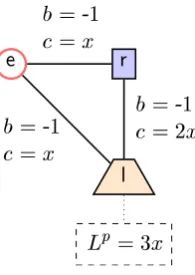
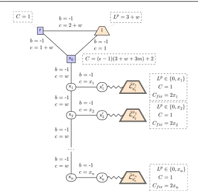
this choice is represented by what we call a choice network. A reduction of an SSP instance consists of the connection of one choice network per element inS and what

we call themain network. We have multiple different choice networks depending on

the problem class and the power flow model. All types of choice networks, except for one, have something in common that: they have one bus which they share with the main network. We call this bus theconnectorand we typically use the symbolefor it.

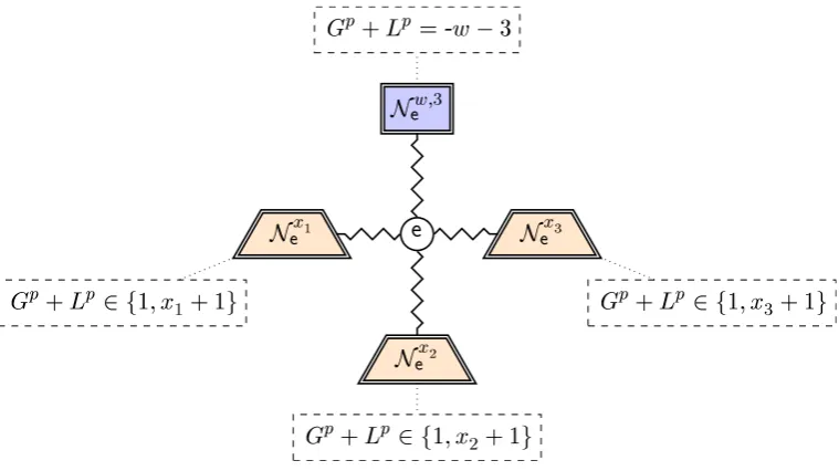
In the following, we present an abstract example of what a reduction of a feasibility problem could look like. We assume the existence of choice networksNex where its superscript indicates a dependency onx. Also, letNew,n be the main network, which depends onwandn. Thereduction networkis defined as_NS,w := _New,n+ePe_x∈SN

x

e. Fig. 3.1 presents networkNS,wfor theSSPinstance(_{x₁, x₂, x_3}, w).

e Nx1

e

Gp+ Lp 2 f1; x₁+ 1g

Nx2 e

Gp_{+ L}p_{2 f1; x} 2+ 1g

Nx3 e

Gp+ Lp 2 f1; x₃+ 1g New;3

[image:36.595.88.468.410.623.2]

Gp+ Lp =-w 3

Figure 3.1: The common pattern found in manySSPbased reductions.

The index on the choice networks e shows that the connector is callede and the zigzag line between a choice network and the bus e show that the buses e are the same. The superscriptx_i indicates that the networks parameters depend onx_i. The

(37)

§3.2 NP-Hardness Reduction 23

flow of1orx_i+ 1. Since the values are positive, we can derive that the network can

only consume power, i.e. it cannot generate power. In other words, it cannot provide any power to the other choice networks and/or the main network. This property will be proven in a lemma by assuming that the bus is generator and load at the same time and showing that in every solution of this network e either generates -1 or -x_i ₋1 (from an inside point of view).

Also connected to the connectore is the main networkNew,nwhere, in our exam-ple,n = 3. The superscript indicates that the parameter of this network depend on w andn. The shape of the main network indicates that it acts as generator and the

annotated values show that it generates a fixed value ofw + 3. Note that in some

cases the main network simply consists of the buseonly. For example, if the problem class allows for a fixed active power generation we can makeea generator and fix its generation tow+n. If the main network is more than just the buse then the fixed generation ofw+nwill be proven in a lemma. In some cases, the main network also

depends onm:=P x∈Sx.

With this pattern, showing NP-hardness works as follows. We call a choice net-workactiveif it consumesx_i+ 1. Otherwise, we call itinactive. There is a one to one

correspondence between the active choice networks of a reduction and the elements of a solution of(S, w). Assume that(S, w)is solvable andV is a solution. We activate

all networksNxi

e withx_i ∈V and keep all other networks inactive. The properties of the choice networks and the property of the main network imply that there are power flow solutions which are consistent within the networks itself. The fact thatV is a

so-lution ensures that Kirchhoff’s junction law for active power ateis satisfied. Hence, the combination of all these solutions is a solution for NS,w. On the other hand, let NS,whave a solution. The lemma about the choice network ensures that every choice

network is either active or inactive. Furthermore, the main network has to generate

w+n. Since we have a solution, Kirchhoff’s junction law atemust be satisfied. Hence, we have

w+n= X

x∈S

Nexactive

(x+ 1) + X

x∈S

Nexinactive 1

w= X

x∈S

Nexactive

x.

Therefore,V :=_{x_{| N}exis active}is a solution of(S, w).

(38)

the AC model, the voltage magnitude ofe has to be fixed. It cannot depend on the value of the parameter (x) or the state of the network (active or inactive). Otherwise

we might not be able to combine the solutions of the choice networks. In one case we prove the properties of the choice network under the assumption that the voltage magnitude ofe is fixed to some valuez . Henceforth, in this case the main network

has to ensure that the voltage magnitude ofeis fixed atz.

3.3 Non-Approximability of OPF

We illustrate how to show that there is no -approximation algorithm for the OPF

problem unless P = NP. The idea presented below works for all flow models. Let (S, w) be an SSP instance. The reduction will be such that the existence of an

-approximation algorithm allows us to decide whether(S, w)is solvable or not. Given that the SSP is NP-complete, the existence of an -approximation algorithm would

hence allow us to decide all problems inNPin polynomial time. However, since we assumeP6=NP, this leads to a contradiction.

In the reduction, we have two types of generators. One which is cheap and one which is expensive. The reduction is such that if theSSPinstance is solvable only the cheap generators will be used. Let the cost of this bey. Note that these costs depend

on w. Also, the reduction has to ensure that y is the lower bound for all possible

solutions.

If the instance is not solvable, then the reduction is such that we have to generate at least one unit of power with the expensive generator. The expensive generator will have cost ofy+ 1. Hence, if the instance was not solvable then we have overall cost

of at leasty+ 1.

Let us assume the existence of an-approximation algorithm. If(S, w)is solvable then the algorithm returns a solution with cost within [y, y]. If the instance is not

solvable then we have cost of at leasty+ 1. Hence, we have that(S, w)is solvable if and only if the cost of the solution returned by the algorithm is less or equal thany.

This shows that the-approximation algorithm decides theSSPinstance. One fur-ther restriction on the reduction is that the size ofy has to be polynomial in the size

the instance(S, w). This is because we need the value ofy to decide solvability. Note

that the size ofdoes not matter. It can be considered a constant because there is only

(39)

Chapter 4

The DC Power Flow Model with

Line Switching

In this chapter, we present the complexity results regarding the Linear AC Approxi-mation of the Alternating Current (AC) power model. This model is also called DC model due to its visual similarity with the flow equations of the direct current. The DC model approximates the AC model by ignoring the reactive power. The model is build on the assumption that we have unity voltage magnitudes. We also assume that the lines are lossless (conductance is 0) and the sine function within the AC power flow is approximated by a linear function (see Section 4.1).

The DC model is a linear model. Its advantage is that if we have a linear objective, we have a Linear Program. This is true for the OPF and the MPF, in the form we study here.

The fact that we can formulate both optimization problems as Linear Programs makes them polynomial to solve in theory (Karmarkar [1984]; Khachiyan [1980]). Sec-tion 4.2 shows that line switching can help improving optimal soluSec-tions for the OPF and MPF. Hence, in this chapter we study the complexity of these problems with additional line switching.

We use the acronym DS for the DC model with line switching. An overview of the results of this chapter is presented in Table 4.1. This table also highlights the features: network structure, maximum bus degree (mD), number of generators (nG) and number of loads (nL).

We begin this chapter by introducing formal definitions of our problems in Sec-tion 4.1. In SecSec-tion 4.2 we present an introductory example of the effects of line switch-ing and aim to clarify the reasons which lead to this behavior. We then present results about the PF in Section 4.3, the OPF in Section 4.4 and the MPF in Section 4.5. In Section 4.6 we conclude the chapter with related work.

4.1 Background

In this section, we present the definitions for the DC and DC switching (DS) problems of MPF, OPF and PF. These definitions are based on the definitions presented in Chapter 2, especially GP networks (Definition 2.3.1). We start by introducing DC

(40)

Problem Result Structure mD nG nL Theorem

DS-PF Polynomial at mostkcycles _∞ _∞ _∞ 4.3.1

DS-PF NP-complete series-parallel 3 1 1 4.3.4

DS-OPF Polynomial at mostkcycles ∞ ∞ ∞ 4.4.1

DS-OPF not APX cacti 3 ∞ ∞ 4.4.4

DS-OPF NP-complete cacti 3 ∞ ∞ 4.4.5

DS-OPF NP-complete series-parallel 3 2 1 4.4.6

DS-MPF Polynomial at mostkcycles ∞ ∞ ∞ 4.5.1

DS-MPF NP-complete cacti 3 ∞ ∞ 4.5.2

DS-MPF NP-complete series-parallel 3 1 1 4.5.3

DS-MPFLp not APX arbitrary ∞ 6 6 4.5.5

DS-MPF stronglyNP-complete planar 3 1 1 4.5.6

Table 4.1: DC Model with Line Switching (DS Model) Result Overview

solutions, which are essentially GP solutions (Definition 2.3.5) where the power flow

follows the DCpower flow law.

Definition 4.1.1(DC solution, congested). LetN = (N , N_G, N_L, E , Gp, Lp)be a GP network. A DC solutionis a tuple(θ, Gp_{, L}p₎ _{such that}₍_{θ, G}p_{, L}p_{, p}₎_{is a GP solution}

wherep:Ed_→

Rand we have to have∀(a,d, b, g, c)∈Ed:

|pad| ≤cand

pad =b(θa−θd).

A line(_{a,d}, b, g, c)_∈E is calledcongestedif_|pad|=c. The set of all DC solutions of

N is denoted withSDC(_N).

We refer topas theimplied flowfrom the DC solution(θ, Gp, Lp). Note that the

con-ductanceg is not used in the definition of DC solutions. Hence, when defining lines

of GP networks within the context of the DC model, we will omit the conductance. Furthermore, we use the following more compact form when defining lines

(_{a,d}, b₁, g₁, c₁) u a

b=b1

←−→_c=c

1 d.

4.1.1 Line Switching

Switching means disconnecting two previously connected buses. When using the

word switching, we always refer to switching lines off, never to switching lines on. This is motivated from the fact that we are always given the network and a solution consists of finding asub-network.

Definition 4.1.2(sub-network). LetN = (N , N_G, N_L, E , Gp, Lp)be a GP network and

(41)

§4.1 Background 27

We callE0theset of switched lines. Aswitching solution(DS solution) is essentially

a DC solution for a sub-network of a given network N. The set of switched lines

becomes part of the solution.

Definition 4.1.3(DS solution). LetN = (N , N_G, N_L, E , Gp, Lp)be a GP network. A DSsolutionis a tuple(E0_{, θ, G}p_{, L}p₎_{such that}_E0 _⊆_E _and₍_{θ, G}p_{, L}p₎_{is a DC solution}

ofNE0

. The set of all DS solutions forN is denoted withSDS(N).

4.1.2 MAXIMUMPOWERFLOW

The DC-MPF returns the maximum demand we can satisfy in a given MPF network (see Definition 2.4.1) whilst satisfying the DC power flow law.

Definition 4.1.4(DC-MPF, DS-MPF). LetN = (N , N_G, N_L, E , Gp, Lp)be a MPF net-work. The DC-MPF ofN is

DC-MPF(N) := max

(θ,Gp_,Lp₎_∈SDC₍_N₎ X

l∈N_L Lp_l.

Given anx _∈Q≥0the DC-MPF problem is to decide whether DC-MPF(N)≥x. The

DS-MPF ofN is

DS-MPF(N) := max

E0_⊆_EDC-MPF(N

E0 ).

Given anx_∈Q≥0the DS-MPF problem is to decide whether DS-MPF(N)≥x.

We are not able to show non-approximability of the DS-MPF as defined above. However, we show non-approximability for a variant of the DS-MPF where a single load is fixed. This variant is called DS-MPFLp.

Definition 4.1.5(DS-MPFLp). LetN = (N , N

G, NL, E , Gp, Lp)be a GP network with N_G_∩N_L=_∅,_|dom(Gp)_|= 0and_|dom(Lp)_|= 1. The DS-MPFLpofN is

DS-MPFLp(N) := max (E0_,θ,Gp_,Lp₎_∈SDS₍N)

X

l∈N_L Lp_l.

4.1.3 OPTIMALPOWERFLOW

The OPF is concerned with assigning values to the generation variables so that the given demand is satisfied and the total generation cost is minimal. Since we have a fixed demand, it is possible that no solution exists. In such a case, the DC-OPF will be infinite.

Definition 4.1.6 (DC-OPF, DS-OPF). LetN = (N , N_G, N_L, E , Gp_{, L}p₎ _{be a GP}

net-work with (N, C)be an OPF network. The DC-OPF ofN is DC-OPF(N, C) := min

(θ,Gp_,Lp₎_∈SDC₍_N₎ X

r∈N_G