Issue 32

00001101

00001010

00001101

00001010

01001100

01101111

01110010

01100101

01101101

00100000

01101000

01110001

01110011

01110101

Issue

32

₂₀₁₈

Computer Vision for the Masses

Up Your Game: Practical Optimizations for Game Programmers

CONTENTS

FE

ATURE

Letter from the Editor

3

Computer Vision: Coming Soon to a Browser Near You

by Henry A. Gabb, Senior Principal Engineer, Intel Corporation

Computer Vision for the Masses

5

Bringing Computer Vision to the Open Web Platform*

Up Your Game

23

How to Optimize Your Game Development―No Matter What Your Role―Using Intel® Graphics Performance Analyzers

Harp-DAAL for High-Performance Big Data Computing

31

The Key to Simultaneously Boosting Productivity and Performance

Understanding the Instruction Pipeline

41

The Key to Adaptability in Modern Application Programming

Parallel CFD with the HiFUN* Solver on the Intel® Xeon® Scalable Processor

51

Maximizing HPC Platforms for Fast Numerical Simulations

ImprovIng VASP* Materials SimulatIon Performance

61

Computer Vision: Coming Soon to a Browser Near You

My first exposure to the field of computer vision was

Gary Bradski’s OpenCV* article in

Dr.

Dobb’s Journal

. Gary was working in Intel Labs at the time. I’d just joined Intel a few months

earlier and was surprised to learn that we were working in that area. OpenCV has come a long

way since its first release 17 years ago. Among other things, it’s open-source and supported

by

OpenCV.org

, a non-profit foundation. In this issue’s feature article,

Computer Vision for

the Masses

, a group of collaborators from the University of California, Irvine, and Intel Labs

describe their work to translate many of OpenCV’s key capabilities to JavaScript* to do

high-performance computer vision within the

Open Web Platform

*. They present compelling

examples of common computer vision applications like edge detection, face recognition,

background subtraction, and image recognition using deep neural networks running within

a browser.

Continuing with graphics and video processing,

Up Your Game

shows how to optimize game

performance using

Intel® Graphics Performance Analyzers

. We present several use cases to

show how different members of a game development team―like artists, designers, gameplay

programmers, and game engine programmers―can take advantage of these analysis tools.

The

Google File System

* and

MapReduce

* ushered in the era of large-scale,

distributed-memory data analytics back in 2003. Since then, many options have become available to

data analytics and machine learning at scale.

Apache Spark

* is my current favorite, but I’ve

experimented with

Dask

*,

HPAT

(the High-Performance Analytics Toolkit project from Intel

Labs), and one or two others. In

Harp-DAAL for High-Performance Big Data Computing

,

Professor Judy Qiu of Indiana University introduces a new framework that takes advantage of

the highly-optimized

Intel® Data Analytics Acceleration Library

. This article describes the

framework and walks you through an example, complete with Java* code, showing how to do

k-means clustering using Harp-DAAL.

LETTER FROM THE EDITOR

Henry A. Gabb, Senior Principal Engineer at Intel Corporation, is a longtime high-performance and

parallel computing practitioner who has published numerous articles on parallel programming. He

From high-level abstractions, we move to the opposite extreme.

Understanding the Instruction

Pipeline

offers a gentle, conceptual overview of the instruction pipeline and why it matters

for performance on modern processors. We close this issue with two articles on boosting

the performance of compute-intensive scientific applications:

Parallel CFD with the HiFUN*

Solver on the Intel® Xeon® Scalable Processor

and

Improving VASP* Materials Simulation

Performance

. The former presents a parallel performance tuning case study using a real fluid

dynamics application. And the latter shows how to generate a concise summary of application

performance using

Intel® VTune™ Amplifier

– Application Performance Snapshot, and describes

an interesting new preview feature in

Intel® MPI Library

.

Future issues of

The Parallel Universe

will bring you articles on doing deep learning within the

Apache Spark analytics framework, Java performance enhancements, profiling and tuning I/O

performance, new features in Intel® Software Development Tools, and much more. Be sure to

subscribe

so you won’t miss a thing.

Henry A. Gabb

Sajjad Taheri, PhD Candidate, Alexeandru Nicolau and Alexeander Vedienbaum, Professors

of Computer Science, University of California, Irvine; Ningxin Hu, Senior Staff Engineer, and

Mohammad Reza Haghighat, Senior Principal Engineer, Intel Corporation

The Web is the world’s most universal compute platform and the foundation for the digital economy. Since its birth in early 1990s, Web capabilities have been increasing in both quantity and quality. But in spite of all the progress, computer vision isn’t yet mainstream on the Web. The reasons include:

• The lack of sufficient performance of JavaScript*, the standard language of the Web

• The lack of camera support in the standard Web APIs

• The lack of comprehensive computer vision libraries

Bringing Computer Vision to the Open Web Platform*

These problems are about to get solved―resulting in the potential for a more immersive and perceptual Web with transformational effects including online shopping, education, and entertainment, among others.

Over the last decade, the tremendous improvements in JavaScript performance, plus the recent emergence of WebAssembly*, close the Web performance gap with native computing. And the HTML5 WebRTC* API has brought camera support to the Open Web Platform*. Even so, a comprehensive library of computer vision algorithms for the Web was still lacking. This article outlines a solution for the last piece of the problem by bringing OpenCV* to the Open Web Platform.

OpenCV is the most popular computer vision library, with a comprehensive set of vision functions and a large developer community. It’s implemented in C++ and, up until now, was not available in Web browsers without the help of unpopular native plugins.

We’ll show how to leverage OpenCV efficiency, completeness, API maturity, and its community’s collective knowledge to bring hundreds of OpenCV functions to the Open Web Platform. It’s provided in a format that’s easy for JavaScript engines to optimize and has an API that’s easy for Web programmers to adopt and use to develop applications. On top of that, we’ll show how to port OpenCV parallel implementations that target single instruction, multiple data (SIMD) units and multiple processor cores to equivalent Web primitives―providing the high performance required for real-time and interactive use cases.

The Open Web Platform

The Open Web Platform is the most universal computing platform, with billions of connected devices. Its popularity in online commerce, entertainment, science, and education has grown exponentially―as has the amount of multimedia content on the Web. Despite this, computer vision processing on Web browsers hasn’t been a common practice. The lack of client-side vision processing is due to several limitations:

• A lack of standard Web APIs to access and transfer multimedia content

• Inferior JavaScript performance

• Lack of a comprehensive computer vision library to develop apps

The approach we outline here, along with other recent developments on the Web front, will address those limitations and empower the Web with proper computer vision capabilities.

Adding Camera Support and Plugin-Free Multimedia Delivery

Recently, the immersive Web with access to virtual reality (VR) and augmented reality (AR) content has begun delivering new, engaging user experiences.

Improved JavaScript* Performance

JavaScript is the dominant language of the Web. Because it’s a scripting language with dynamic typing, its performance is inferior to that of native languages such as C++. Multimedia processing often involves complex algorithms and massive amounts of computation. With client-side technologies such as just-in-time (JIT) compilation, and with the introduction of WebAssembly* (WASM*), a portable, binary format for the Web, Web clients can reach a near-native performance with JavaScript and handle more demanding tasks.

A Comprehensive Computer Vision Library

Although there are several computer vision libraries developed in native languages such C++, they can’t be used in browsers without relying on unpopular browser extensions, which pose security and portability issues. There have been a few efforts to develop computer vision libraries in JavaScript, but these are limited to select categories of vision functions. Expanding those efforts with new algorithms, and optimizing the implementation, are challenging tasks. Previous work lacked either functionality, performance, or portability.

As an alternative approach, we take advantage of an existing comprehensive computer vision library developed in C++ (i.e., OpenCV) and make it work on the Web. This approach works great on the Web for several reasons:

• It provides an expansive set of functions with optimized implementation.

• It performs more efficiently than normal JavaScript implementations, and performance will further improve through parallelism.

• Developers can access a large collection of existing resources such as tutorials and examples.

OpenCV.js*

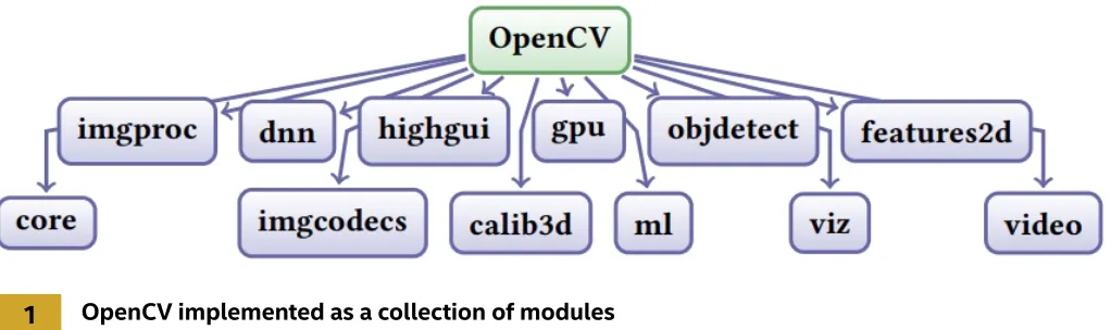
OpenCV1 _{is the de facto library for computer vision development. It’s an open-source library that started}

at Intel Labs back in 2000. OpenCV is very comprehensive and has been implemented as a set of modules (Figure 1). It offers a large number of primitive kernels and vision applications, ranging from image

Table 1. OpenCV.js provided functionalities

Module Provided Function

Core components Image manipulation and basic arithmetic

Image processing Numerous functions to process and analyze images

Image processing Video processing algorithms such as tracking, background segmentation, and optical flow

Object detection HAAR*- and HOG*-based cascade classifiers

DNN Inference of trained Caffe*, Torch*, or TensorFlow* models

GUI features Helper functions to access frames from HTML Canvas*, video elements, and

cameras

1

Table 1 categorizes and lists the functions currently included in OpenCV.js. It omits several OpenCV modules, for two reasons:

1. Not all of OpenCV’s offerings are suitable for the Web. For instance, the high-level GUI and I/O module

(highgui)―which provides functions to access media devices such as cameras and graphical user interfaces― is platform-dependent and can’t be compiled to the Web. Those functions, however, have alternatives using HTML5 primitives, which are provided by a JavaScript module (utils.js). This works, for instance, to access files hosted on the Web and media devices through getUserMedia and to display graphics using HTML Canvas*.

2. Some of the OpenCV functions are only used in certain application domains that aren’t common in typical Web applications. For instance, the camera calibration module (calib3d) is often used in robotics. To reduce the size of the generated library for general use cases, based on OpenCV community feedback, we have identified the least commonly used functions from OpenCV and excluded them from the JavaScript version of the library.

Translating OpenCV to JavaScript* and WebAssembly*

The emergence of Emscripten*2_{, an LLVM-based source-to-source compiler developed by Mozilla, has made} it possible to port many programs and libraries developed in C++ to the Web. Originally, Emscripten targets a typed subset of JavaScript called asm.js that, because of its simplicity, allows JavaScript engines to perform extra levels of optimization. In fact, it’s even possible to compile asm.js functions before execution.

While performance is impressive, parsing and compiling large JavaScript files could become a bottleneck, especially for mobile devices with weaker processors. This was one of the main motivations for development of WASM3_{. WASM is a portable size- and load-time-efficient binary format designed as a target for Web} compilation. We used Emscripten to compile OpenCV source code into both asm.js and WASM. They offer the same functionality and can be used interchangeably.

During compilation with Emscripten, the C++ high-level language information such as class and function identifiers are replaced with mangled names. Since it’s almost impossible to develop programs through mangled names, we provide binding information of different OpenCV entities such as functions and classes and expose them to JavaScript. This enables the library to have a similar interface to normal OpenCV, with which many programmers are already familiar. Since OpenCV is large, and grows continuously through new contributions, continuously updating the port by hand is impractical. So we developed a semi-automated approach that takes care of the tedious parts of the translation process while allowing expert insights that can enable high-quality, efficient code production.

2

Using OpenCV.js in Web Applications

Let’s explore how to use OpenCV.js to develop Web applications. Figure 3 shows an overview of OpenCV.js and its interaction with Web applications. Web applications will use the OpenCV.js API to access the functions as listed in Table 1. While the vision functions from OpenCV are compiled either into WASM or asm.js, we have developed a JavaScript module that provides GUI features and media capture. OpenCV.js utilizes standard Web APIs, such as Web workers and SIMD.js, to achieve high performance, and Canvas and WebRTC* to provide media and GUI capabilities.

The OpenCV.js API is inspired by the OpenCV C++ API and shares many similarities with it. For instance, C++ functions are exported to JavaScript with the same name and signature. Function overloading and default parameters are also supported in the JavaScript version. This makes migration to JavaScript easier for users who are already familiar with OpenCV development in C++.

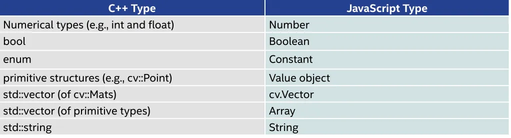
Although OpenCV C++ classes are ported to JavaScript objects with the same member functions and

Table 2. Exported JavaScript types for basic C++ types

C++ Type JavaScript Type

Numerical types (e.g., int and float) Number

bool Boolean

enum Constant

primitive structures (e.g., cv::Point) Value object

std::vector (of cv::Mats) cv.Vector

std::vector (of primitive types) Array

std::string String

3

We’ll present several examples to demonstrate various computer vision tasks using OpenCV.js. All of these examples work on top of a simple HTML Web page. We only present the logic part of the programs that deal with the OpenCV.js API.

Figure 4 shows how to apply the Canny algorithm to find the edges in an image. Input images will be loaded from an HTML Canvas. For this purpose, we’ve provided a helper function that takes the Canvas name and returns a color image. Since the Canny algorithm works on grayscale images, we have to do the extra step at line 3 to invoke cv.cvtColor to convert the input image from color to grayscale. Finally, after getting the result of Canny algorithm, we can render the image in the output canvas (line 6). Figure 5

1 let src = cv.imread (‘canvasInput’); 2 let dst = new cv.Mat ();

3 cv.cvtColor (src, src, cv.COLOR_RGB2GRAY, 0); 4 // You can try more different parameters 5 cv.Canny (src, dst, 50, 100, 3, false); 6 cv.imshow (‘canvasOutput’, dst );

7 src.delete (); dst.delete ();

5

The next example (Figures 6 and 7) uses Haar cascades to detect faces in an image. Since this algorithm works on grayscale images, the input image is converted at line 3. At line 7, we initialize a cascade classifier and load it with a model for detecting faces. Other models trained to detect different objects, such as cats and dogs, can be used as well. At line 9, we invoke detectMultiscale, which searches in multiple copies of input images scaled with different sizes. When finished, it returns a list of rectangles for possible faces in the image. At line 10, we iterate over those rectangles and use the cv.rectangle

function to highlight that part of the image.

6

We’ve seen how to process single images in Web applications using OpenCV.js. Processing video boils down to processing a sequence of individual frames. The next example (Figures 8 and 9) demonstrates:

• How to capture frames from a video element

• How to subtract background from input video using the MOG2 algorithm

• How to display the processed frame on an HTML Canvas

The cv.VideoCapture object provided by utils.js enables WebRTC to access and manage camera resources. This examples assumes the input video contains 30 frames per second. So, at every 1/30 of a second, it invokes the processVideo function. This function:

• Reads the next video frame (line 18)

• Applies background extraction function (line 19)

• Displays the output foreground mask (line 20)

1 let src = cv.imread (‘canvasInput’); 2 let gray = new cv.Mat();

3 cv.cvtColor (src, gray, cv.COLOR_RGBA2GRAY, 0); 4 let faces = new cv.RectVector ();

5 let faceCascade = new cv.CascadeClassifier ();

6 // load pre-trained classifiers

7 faceCascade.load (‘haarcascade_frontalface_default.xml’); 8 // detect faces

9 faceCascade.detectMultiScale (gray, faces); 10 for (let i = 0; i < faces.size(); ++i) { 11 let roiGray = gray.roi (faces.get(i)); 12 let roiSrc = src.roi (faces.get(i));

13 let point1 = new cv.Point (faces.get(i).x, faces.get(i).y); 14 let point2 = new cv.Point (faces.get(i).x + faces.get(i).width, 15 faces.get(i).y + faces.get(i).height);

16 cv.rectangle (src, point1, point2, [255, 0, 0, 255], 3); 17 roiGray.delete (); roiSrc.delete ();

18 }

19 cv.imshow (‘canvasOutput’, src);

20 src.delete (); gray.delete (); faceCascade.delete (); 21 faces.delete ();

8

1 let video = document.getElementById (‘videoInput’);

2 let cap = new cv.VideoCapture (video);

3

4 let frame = new cv.Mat (video.height, video.width, cv.CV_8UC4);

5 let fgmask = new cv.Mat (video.height, video.width, cv.CV_8UC1);

6 let fgbg = new cv.BackgroundSubtractorMOG2 (500, 16, true); 7

8 const FPS = 30;

9 function processVideo () { 10 try {

11 if (! streaming) { 12 // clean and stop

13 frame.delete (); fgmask.delete (); fgbg.delete (); 14 return;

15 }

16 let begin = Date.now (); 17 // start processing 18 cap.read (frame);

19 fgbg.apply (frame, fgmask);

20 cv.imshow (‘canvasOutput’, fgmask); 21 // schedule the next one

22 let delay = 1000/FPS - (Date.now () - begin); 23 setTimeout (processVideo, delay);

24 } catch (err) {

25 utils.printError (err); 26 }

27 };

28 // schedule the first frame

29 setTimeout (processVideo, 0);

The last example (Figures 10 and 11) demonstrates using a pre-trained DNN in Web applications. While in this example we use a DNN to recognize objects, they can also be specialized to do other recognition tasks, such as background segmentation. At line 2, the program reads a Caffe framework model of GoogleNet*. Other formats, such as Torch and TensorFlow, are also supported. In the next step, at line 6, we convert the input image into a blob that fits the network. Then, at lines 9 and 10, we forward the blob along the network and find the highest probability class. Figure 10 shows a snapshot of the program categorizing a sample image. (You can see more examples of OpenCV.js usage at https://docs.opencv.org.)

1 let src = cv.imread (‘canvasInput’);

2 let net = cv.readNetFromCaffe (‘bvlc_googlenet.prototxt’, 3 ‘bvlc_googlenet.caffemodel’); 4 if (net.empty ());

5 throw “Failed to read net”;

6 let inputBlob = cv.blobFromImage (src, 1, new cv.Size (224, 224), 7 new cv.Scalar (104, 117, 123)); 8

9 net.setInput (inputBlob, data); 10 let prob = net.forward (“prob”); 11 let minMax = cv.minMaxLoc (prob); 12

13 console.log (“Best class: #” + minMax.maxLoc.x + “ “ +

14 keywords [minMax.maxLoc.x] + “Probability: “ + minMax.maxVal); 15

16 prob.delete (); inputBlob.delete (); 17 net.delete (); src.delete ();

Performance Evaluation

OpenCV.js brings a lot of computer vision capabilities to the Web. To demonstrate their performance, we have selected a number of vision benchmarks including primitive kernels and more sophisticated vision applications including:

• Canny’s algorithm for edge detection

• Finding faces using Haar cascades

• Finding people using a histogram of gradients

We used a Firefox* browser running on an Intel® Core™ i7-3770 processor with 8GB of RAM with Ubuntu* 16.04 for our setup and ran experiments over sequences of videos.

Figure 12 shows the average speedup of both simple JavaScript kernels and vision applications compared to their native equivalent that use an OpenCV scalar build (i.e., not using parallelism). As you can see, the JavaScript performance is competitive. While we found WASM and asm.js performance to be close, the WASM version of the library is significantly faster to initialize and is more compact. Its size is about 5.3 MB compared to the asm.js version, which is 10.4 MB.

Making it Even Faster

Computer vision is computationally demanding. A lot of computations need to be performed on a massive number of pixels. For instance, each iteration of the baseline Canny, face, and people benchmarks takes on average 7 ms, 345 ms, and 323 ms, respectively, to process a single 800 x 600 resolution image. While it’s fast to compute Canny, face, and people detection, they are still very expensive and cannot be used in real-time, interactive use-cases.

Fortunately, computer vision algorithms are inherently parallel, and good algorithm design and an optimized implementation can lead to significant speedups on parallel hardware. OpenCV comes with parallel implementations of algorithms for different architectures. We take advantage of two methods that target multicore processors and SIMD units to make the JavaScript version faster. We’ve skipped GPU implementations at the moment due to their complexity. The upcoming WebGPU* API can potentially be used to accelerate OpenCV on GPUs.

SIMD.js

SIMD.js4, 5 _{is a new Web API to expose processor vector capabilities to the Web. It is based on a common} subset of the Intel SSE2 and ARM NEON* instruction sets that runs efficiently on both architectures. They define vector instructions that operate on 128-bit-wide vector registers, which can hold four integers, four single-precision floating-point numbers, or 16 characters. Figure 13 shows how vector registers can add four integers with one CPU instruction.

SIMD is proven to be very effective in improving performance, especially for multimedia, graphics, and scientific applications.5, 6 _{In fact, many OpenCV functions, such as core routines, are already implemented} using vector intrinsics. We’ve adapted the work done by Peter Jensen, Ivan Jibaja, Ningxin Hu, Dan Gohman, and John Mc-Cutchan7 _{to translate OpenCV vectorized implementations using SSE2 intrinsics} into JavaScript with SIMD.js instructions. Inclusion of the SIMD.js implementation will not affect the library interface. Figure 14 shows the speedups that are obtained by SIMD.js on selected kernels and applications running on Firefox. Up to 8x speedup is obtained for primitive kernels. As expected, the speedup is higher for smaller data types. There are fewer vectorization opportunities in complex functions such as Canny, face, and people detection. Currently, SIMD.js can only be used in the asm.js context and is supported by the Firefox and Microsoft Edge* browsers. SIMD in WebAssembly is currently planned to have the same specification as SIMD.js. Hence, similar performance numbers are expected.

14

Multithreading using Web Workers

JavaScript programs use Web workers for parallel processing of heavy computing tasks. Web workers communicate by message passing, which could incur significant cost, especially when passing large messages such as images. SharedArrayBuffer8 _{has recently been proposed as a storage system} that can be shared between Web workers. They can use it to implement a shared-memory parallel

API into equivalent JavaScript using Web workers with shared array buffers. OpenCV.js with

multithreading support will use a pool of Web workers and allocate a worker when a new thread is being spawned. Also, it exposes OpenCV APIs to dynamically adjust the concurrency such as changing number of concurrent threads (i.e., cv.SetNumThreads) to JavaScript.

To study the performance impact of using multiple Web workers, we measured the performance of three application benchmarks that did not gain significantly from SIMD vectorization using different numbers of workers (up to 8). The OpenCV load balancing algorithm divides the workload evenly among threads. As shown in Figure 15, on a processor with eight logical cores, we obtained a 3x to 4x speedup. Note that a similar trend is observed on native Pthreads implementations of the same functions.

15

Computer Vision for the Masses

as Electron*. Combined with the recent developments in Web platform, it’s a more efficient way to make real new Web applications and experiences like emerging virtual and augmented reality. We’ve also provided a large collection of computer vision tutorials using OpenCV.js that we hope will be a good asset for education and research purposes.

The authors are grateful to Congxiang Pan, Gang Song, and Wenyao Gan for their contributions through the Google Summer of Code program, and would also like to thank the OpenCV founder, Dr. Gary Bradski, its chief architect, Vadim Pisarevsky, and Alex Alekin for their support and helpful feedback.

Learn More

We’ve developed extensive online resources to help developers and researchers learn more about OpenCV.js and computer vision in general:

• OpenCV.js documentation and tutorials • OpenCV.js demos

OpenCV.js can also be used in Node.js-based environments. It’s published on the Node Package Manager (NPM) at https://www.npmjs.com/package/opencv.js.

References

1. Gary Bradski and Adrian Kaehler. Learning OpenCV: Computer vision with the OpenCV library. O’Reilly Media, Inc., 2008.

2. Alon Zakai. Emscripten: An LLVM-to-JavaScript compiler. In Proceedings of the ACM international

conference companion on Object oriented programming systems languages and applications companion, pages 301–312. ACM, 2011.

3. Andreas Haas, Andreas Rossberg, Derek L Schuff, Ben L Titzer, Michael Holman, Dan Gohman, Luke Wagner, Alon Zakai, and JF Bastien. Bringing the Web up to speed with WebAssembly. In Proceedings of the 38th ACM SIGPLAN Conference on Programming Language Design and Implementation, pages 185– 200. ACM, 2017.

4. SIMD.js specification: http://tc39.github.io/ecmascript_simd/. 2017.

5. Ivan Jibaja, Peter Jensen, Ningxin Hu, Mohammad R Haghighat, John McCutchan, Dan Gohman, Stephen M Blackburn, and Kathryn S McKinley. Vector parallelism in JavaScript: Language and compiler support for SIMD. In Parallel Architecture and Compilation (PACT), 2015 International Conference on, pages 407–418. IEEE, 2015.

6. Sajjad Taheri. Bringing the power of simd.js to gl-matrix: https://hacks.mozilla.org/2015/12/bringing-the-power-of-simd-js-to-gl-matrix/. 2015.

7. Peter Jensen, Ivan Jibaja, Ningxin Hu, Dan Gohman, and John Mc-Cutchan. SIMD in JavaScript via C++ and Emscripten. In Workshop on Programming Models for SIMD/Vector Processing, 2015.

up YOuR GaME

Giselle Gomez, Technical Consulting Engineer, Intel Corporation

Performance optimization can mean the difference between a good game and a great game. And providing that smooth playing experience can be a daunting task. But Intel® Graphics Performance Analyzers (Intel® GPA) can help streamline the process, making it possible for everyone on your development team to lend a helping hand. After reading this article, you’ll be able to pinpoint exactly where you fit into the optimization process and see how the Intel GPA tool suite can help you reach your optimization goals, like higher fidelity or better framerate.

Where Do You Fit?

There are three main types of game developers:

1. Artists/designers 2. Gameplay programmers 3. Game engine programmers

How to Optimize Your Game Development―No Matter What Your Role―

Each of these groups plays a vital role. And each interacts with the optimization process in a different way. Let’s dive into some use cases to better understand the differences.

Artists/Designers

We’ll begin with the artists who create the assets associated with characters and the environment within the game―the scenery, objects, surface textures, vehicles, etc.

To create the best viewing experience, artists typically develop these elements with the highest fidelity in mind (4K textures and more complex geometry), but they can be scaled back during optimization. Artists work to create textures and assets that allow for smooth gameplay on the target hardware. They also work hand-in-hand with gameplay programmers to execute design ideas relating to lighting, movement, and overall design execution.

When you’re retargeting for a new minimum specification or optimizing due to inadequate framerate, you can run into issues like:

• Texture bandwidth: Textures that are too big or too high-resolution

• Geometric complexity: Polygons that are very small

Optimization tools like Intel GPA allow artists to self-check their work, ensuring that any texture or asset addition doesn’t drop the framerate below your target or cause additional gameplay issues.

1

increase for the entire frame (1). This shows it might be beneficial to view the used textures for the

selected draw call and consider using a lower MIP level for the textures, if they don’t drastically

impact the final scene quality.

Gameplay Programmers

2

ap-pear in the left-hand side of the resource viewer, if there are different MIPs associated with that texture. From here, you can see how the texture will affect the scene and final render target.

During optimization, these programmers focus their attention on efficient code performance to create a good base layer for assets. The more efficient the back-end code is, the better. When these programmers use Intel GPA, the main benefit they’ll see is in live editing with playback, CPU/GPU profiling, and experiments (although this list of benefits is not exhaustive by any means).

Intel GPA offers multiple ways to determine where and when to optimize code or to optimize the way in which objects are rendered (the number of objects and batching). One common area a gameplay

3

• How particle effects are rendered

• The lighting (reflection, number of lights, etc.) • How objects are placed within a scene

• How draw calls are batched (dynamic batching versus static batching)

Another quick optimization is to look through the API log to determine if there are any duplicate draw calls, or in the bar chart to determine if there are duplicate passes like an additional depth pass. The tool gameplay

programmers will initially use during optimization, however, is the Trace Analyzer tool. Capturing a trace during live analysis opens the door to profiling CPU and GPU utilization. Once open, a trace shows the CPU and GPU queue, frame timings, V-Sync, and process duration. Trace Analyzer is also customizable, allowing a user to change which metrics are collected during capture. By viewing where waits happen, how long an item is in the

4

Game Engine Programmers

Finally, we come to the game engine programmers, who create a tool that enables the gameplay programmers to complete their job. The game engine programmers create game-agnostic components that are the

foundation on which the gameplay programmers create the game. This can include:

• Implementing how animations will happen

• The physics behind gameplay

• Collision detection

• How pixels will be rendered to the screen

As we touched on in the gameplay programmers section, without dedicated game engine programmers, the gameplay programmers would optimize the shaders. However, with the addition of game engine programmers, shader optimization (vertex, pixel, compute, etc.) falls to the game engine programmers. Using the overdraw view in Frame Analyzer, programmers can identify any Z-test- or depth-test-related optimizations. By entering the overdraw view (Figure 5) for a render target, a programmer can identify whether or not the engine is currently rejecting pixels that will be hidden by closer objects within the scene. If there’s significant overdraw in a scene, it might be useful to further investigate and determine if the depth test is being used within the engine. Adding Z-rejection could limit the number of times an unseen pixel is fully rendered, reducing the total number of draw calls for any given scene. Game engine programmers would also touch any other aspects of the rendering pipeline during optimization, as well as using Trace Analyzer to inspect CPU/GPU utilization and determine any optimizations needed on the CPU, such as optimizing the AI algorithm and physics

computations. Game engine programmers can use every aspect of Intel GPA from the GPU pipeline view, which identifies GPU pipeline bottlenecks, to the buffer views.

To learn more on practical optimizations for game engine engineers using Intel GPA, go to Practical Game Performance Analysis Using Intel® Graphics Performance Analyzers (though please note, this article is written using the old UI of Intel GPA), or watch this video.

From Good Game to Great Game

BuILD BETTER,

FasTER CODE

Get Intel’s powerful performance libraries to optimize

your code and cut your development time. They’re

free as part of Intel’s mission to support innovation

and impressive performance on Intel® architecture.

FREE DOwnLOaD >

Judy Qiu, Intelligent Systems Engineering Department, School of Informatics, Computing,

and Engineering, Indiana University

Large-scale data analytics is revolutionizing many business and scientific domains. And easy-to-use, scalable parallel techniques are vital to process big data and gain meaningful insights. This article introduces a novel high-performance computing (HPC)-cloud convergence framework named Harp-DAAL and demonstrates how the combination of big data (Hadoop*) and HPC techniques can simultaneously boost productivity and performance.

Harp* is a distributed Hadoop-based framework that orchestrates node synchronization1_{. Harp uses Intel®}

Data Analytics Acceleration Library (Intel® DAAL)2 _{for its highly-optimized kernels on Intel® Xeon® and}

Xeon Phi™ processor architectures. This way, the high-level API of big data tools can be combined with intra-node, fine-grained parallelism that’s optimized for HPC platforms.

The Key to Simultaneously Boosting Productivity and Performance

We illustrate this framework in detail with K-means clustering, a compute-bound algorithm used in image clustering. We also show the broad applicability of Harp-DAAL by discussing the performance of three other big data algorithms:

1. Subgraph Counting by color coding 2. Matrix Factorization

3. Latent Dirichlet Allocation

These algorithms share characteristics such as load imbalance, irregular structure, and communication issues that create performance challenges.

The categories in Figure 1 illustrate a classification of data-intensive computation into five models that map into five distinct system architectures. It starts with Sequential, followed by centralized batch architectures corresponding exactly to the three forms of MapReduce: Map-Only, MapReduce, and Iterative MapReduce. Category five is the classic Message Passing Interface (MPI) model.

Interfacing Harp and Intel DAAL

Intel DAAL provides a native C/C++ API but also provides interfaces to higher-level programming languages such as Java* and Python*. Harp is written in Java and extended from the Hadoop ecosystem, so Java was the natural choice to interface Harp and Intel DAAL.

In Harp-DAAL, data is stored in a hierarchical data structure called Harp-Table, which consists of tagged partitions. Each partition contains a partition ID (metadata) and a user-defined serializable Java object such as a primitive array. When doing communication, data is transferred among distributed cluster nodes via Harp collective communication operations. When doing local computation, data moves from Harp-Table (JVM heap memory) to Intel DAAL native kernels (off-JVM heap memory). Copying data between a Java object and C/C++ allocated memory space is unavoidable. Figure 2 illustrates two approaches to this data copy:

1. Direct Bulk Copy: If an Intel DAAL kernel allocates a continuous memory space for dense problems, Harp-DAAL will launch a bulk copy operation between a Harp-Table and a native memory address.

2. Multithreading Irregular Copy: If an Intel DAAL kernel uses an irregular and sparse data structure―which means the data will be stored in non-consecutive memory segments―Harp-DAAL performs a second copy operation using Java/OpenMP threads, where the threads transfer data segments concurrently.

Applying Harp-DAAL to Data Analytics

K-means is a widely-used and relatively simple clustering algorithm that provides a clear example of how to use Harp-DAAL. K-means uses cluster centers to model data and converges quickly via iterative refinement. K-means clustering was performed on a large image dataset from Flickr*, which includes 100 million images, each with 4,096 dimensional deep features extracted using a deep convolutional neural network model trained on ImageNet*. Data preprocessing includes format transformation and dimensionality reduction from 4,096 to 128 using Principal Component Analysis (PCA). (The Harp-DAAL tutorial contains a description of the data preparation.)3

Harp-DAAL provides modular Java functions for developers to customize the K-means algorithm as well as tuning parameters for end users. The programming model consists of map functions linked by collectives. The K-means example takes seven steps.

Step 1: Load Training Data (Feature Vectors) and Model Data (Cluster Centers)

// create a pointArray

List<double[]> pointArrays = LoadTrainingData();

Similarly, create a Harp table object cenTable and load centers from HDFS. Since centers are requested by all the mappers, the master mapper will load and broadcast them to all other mappers. Different center initialization methods can be supported in this fashion:

// create a table to hold cluster centers

Table<DoubleArray> cenTable = new Table<>(0, new DoubleArrPlus());

if (this.isMaster()) { createCenTable(cenTable); loadCentroids(cenTable); }

// Bcast centers to other mappers

Step 2: Convert Training Data from Harp to Intel DAAL

The training data loaded from HDFS is stored in the Java heap memory. To invoke the Intel DAAL kernel, this step converts the data to an Intel DAAL NumericTable, which includes allocating the native memory for the NumericTable and copying data from pointArrays to trainingdata_daal.

// convert training data from Harp to DAAL

NumericTable trainingdata_daal = convertTrainData(pointArrays);

Step 3: Create and Set Up an Intel DAAL K-means Kernel

Intel DAAL provides Java APIs to invoke native kernels for K-means on each node. It is called with:

• A specification of the input training data object

• The number of centers

• The number of threads to be used by the thread scheduler (Intel® Threading Building Blocks and Intel® Math Kernel Library)

// create a DAAL K-means kernel object

DistributedStep1Local kmeansLocal = new DistributedStep1Local(daal_Con-text, Double.class, Method.defaultDense, this.numCentroids);

// set up input training data

kmeansLocal.input.set(InputId.data, trainingdata_daal); // specify the number of threads used by DAAL kernel Environment.setNumberOfThreads(numThreads);

// create cenTable on DAAL side

NumericTable cenTable_daal = createCenTableDAAL();

Step 4: Convert Center Format from Harp to Intel DAAL

The centers are stored in the Harp table cenTable for inter-process (mapper) communication. The centers are converted to Intel DAAL format at each iteration.

// Convert center format from Harp to DAAL

Step 5: Local Computation by Intel DAAL Kernel

// specify cluster centers to DAAL kernel

kmeansLocal.input.set(InputId.inputCentroids, cenTable_daal);

// first step of local computation by using DAAL kernels to get a partial result

PartialResult pres = kmeansLocal.compute();

Step 6: Inter-Mapper Communication

Harp-DAAL K-means uses an AllReduce computation model where each mapper keeps a local copy of the whole model data (cluster centers). However, Harp provides different communication operations to synchronize model data among mappers:

• regroup & allgather (default)

• allreduce

• broadcast & reduce • push & pull

In a regroup & allgather operation, it first combines the same center from different mappers and redistributes them to mappers by a specified order. After averaging the centers, an allgather operation makes every mapper get a complete copy of the averaged centers.

comm_regroup_allgather(cenTable, pres);

In an allreduce operation, the centers are reduced and copied to every mapper. Then, on each mapper, an average operation is applied to the centers:

comm_allreduce(cenTable, pres);

At the end of each iteration, call printTable to check the clustering result:

// for iteration i, print the first ten centers of the first ten dimensions

Step 7: Release Memory and Store Cluster Centers

After all of the iterations, release the memory allocated for Intel DAAL and for the Harp table object. The center values are stored on HDFS as the output:

// free memory and record time cenTable_daal.freeDataMemory(); trainingdata_daal.freeDataMemory(); // Write out the cluster centers if (this.isMaster()) {

KMUtil.storeCentroids(this.conf, this.cenDir, cenTable, this.cenVecSize, “output”);

}

cenTable.release();

Performance Results

The performance for Harp-DAAL is illustrated by the results for four applications4,5 _{with different} algorithmic features:

1. K-means: A dense clustering algorithm with regular memory access

2. MF-SGD (Matrix Factorization for Stochastic Gradient Descent): A dense recommendation algorithm with irregular memory access and large model data

3. Subgraph Counting: A sparse graph algorithm with irregular memory access

4. Latent Dirichlet Allocation (LDA): A sparse, topic modeling algorithm with large model data and irregular

memory access

The testbed has two clusters:

1. One with Intel Xeon E5 2670 processors and the InfiniBand Interconnect* 2. One with Intel Xeon Phi 7250 processors and the Intel® Omni-Path Interconnect

Harp-DAAL subgraph counting on 16 Intel Xeon E5 processor-based nodes has a 1.5x to 4x speedup over MPI-Fascia for large subtemplates with billion-edged Twitter graph data. The performance improvement comes from node-level pipeline overlapping of computation and communication. Single-node thread concurrency improved by neighbor list partitioning of the graph vertex.

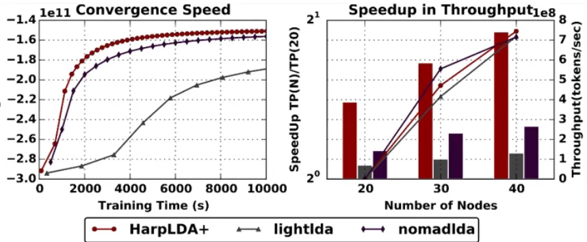
Figure 4 shows that Harp LDA achieves better convergence and speedup over other state-of-the-art MPI implementations such as LightLDA* and NomadLDA*5_{. This advantage comes from two optimizations for} parallel efficiency:

1. Harp adopts the rotation computation model for inter-node communication of the latest model, and at the same time utilizes timer control to reduce the overhead of synchronization.

2. At the intra-node level, a dynamic scheduling mechanism is developed to mitigate load imbalance.

3

The current Harp-DAAL system provides 13 distributed data analytics and machine learning algorithms leveraging the local computation kernels like K-means from the Intel DAAL 2018 release. In addition, Harp-DAAL is developing its own data-intensive kernels. This includes the large-scale subgraph counting algorithm given above, which can process a social network Twitter graph with billions of edges and

subtemplates of 10 vertices in 15 minutes. The Harp-DAAL framework and machine learning algorithms are publicly accessible5 _{so you can download the software, explore the tutorials, and apply Harp-DAAL to other} data-intensive applications.

References

1. Harp code repository, https://github.com/DSC-SPIDAL/harp

2. Intel DAAL, https://github.com/intel/daal

3. Harp-DAAL tutorial, https://github.com/DSC-SPIDAL/harp/tree/tutorial

4. Langshi Chen et. al, Benchmarking Harp-DAAL: High Performance Hadoop on KNL Clusters, in the Proceedings of the 10th IEEE International Conference on Cloud Computing (IEEE Cloud 2017), June 25-30, 2017.

5. Bo Peng et. al, HarpLDA+: Optimizing Latent Dirichlet Allocation for Parallel Efficiency, the IEEE Big Data 2017 conference, December 11-14, 2017.

InTEL® DaTa anaLYTICs aCCELERaTIOn LIBRaRY

HOw’D THEY DO THaT?

Developers worldwide have upped the ante for

application performance, scalability, and portability

with Intel® Software Development Tools.

And they’re sharing their stories

to help you do the same.

Alex Shinsel, Technical Consulting Engineer, Intel Corporation

Understanding the instruction pipeline, on at least a basic level, is as critical to achieving high efficiency in modern application programming as understanding color theory is to painting. It’s a fundamental and ubiquitous concept. While sources vary on exact dates and definitions, instruction pipelining as we know it started gaining popularity at some point in the 1970s or 1980s and is omnipresent in modern machines.

Processing an instruction isn’t instantaneous. There are several steps involved. While the exact details of implementation vary from machine to machine, conceptually it boils down to five main steps:

The Key to Adaptability in Modern Application Programming

1. Fetching an instruction 2. Decoding it

3. Executing it 4. Accessing memory 5. Writing back the results

Without pipelining, each instruction is processed from start to finish before moving on to the next. If we assume that each of the five steps takes one cycle, then it would take 15 cycles to process three instructions (Figure 1).

1

Because each step is handled by a different section of hardware, modern processors improve efficiency by pipelining the instructions, allowing the various hardware sections to each process a different instruction simultaneously. For instance, in cycle 3 of Figure 2, the processor is fetching instruction C, decoding instruction B, and executing instruction A. All three instructions are completed by the end of cycle seven―eight cycles sooner than if they’d been processed sequentially.

We can compare this to washing a second load of laundry while your first load is in the dryer. While processing an instruction certainly involves more steps than doing laundry, we can still divide it into two sections:

• The Front End, the part of the CPU that fetches and decodes instructions

2

Of course, Figure 2 is an oversimplification of instruction pipelining. In reality, the number of steps in the pipeline varies among implementations, with each of the steps used in the example often being split into multiple substeps. However, this doesn’t affect conceptual understanding, so we’ll continue to use the simplified five-step model. Also, this simplified model doesn’t take into account superscalar design, which results in multiple pipelines per processor core because it duplicates functional units such as arithmetic logic units (ALUs) and fetches multiple instructions at once to keep the extra units busy.

The number of pipelines available is called the width. Figure 3 represents a two-wide design that

fetches instructions A and B on the first cycle, and instructions C and D on the second cycle. The width is (theoretically) defined in terms of how many instructions can be issued each cycle, but this is somewhat complicated by the way pipelining is done with CISC designs such as the ever-popular x86.

3

• Slow instructions can bog down the pipeline.

• Complicated instructions may be more likely to stall on data dependencies.

The solution to this problem was to break down these complex operations into smaller micro-operations, or μops. For convenience, the μ is often replaced with u―thus, the uop. The x86 instructions are therefore fetched and decoded, converted into uops, and then dispatched from a buffer to be executed and,

ultimately, retired. This disconnect between x86 instructions being fetched and uops being dispatched makes it hard to define the width of a processor using this methodology, and this difficulty is exacerbated by the fact that pairs of uops can sometimes be fused together.

The concept of the pipeline slot is useful for application optimization because each slot can be classified into one of four categories on any given cycle based on what happens to the uop it contains (Figure 4). Each pipeline slot category is expected to fall within a particular percentage range for a well-tuned application of a given type (e.g., client, desktop, server, database, scientific). A tool like Intel® VTune™ Amplifiercan help to measure the percentage of pipeline slots in an application that fall into each category, which can be compared to the expected ranges. If a category other than Retiring exceeds the expected range for the appropriate application type, it indicates the presence and nature of a performance bottleneck.

4

Much has already been written on the technique of using these measurements for performance

optimization, including the Intel VTune Amplifier tuning guides, and these methods are outside the scope of this article, so we won’t cover them here. (See the suggested readings at the end of this article for additional tuning advice.) Instead, we’ll focus on understanding what’s going on within the pipeline in these situations. For the sake of simplicity, our diagrams will have only a single pipeline.

We’ve already discussed the Retiring category. It represents normal functionality of the pipeline, with no stalls or interruptions. The Back-End-Bound and Front-End-Bound categories, on the other hand, both represent situations where instructions weren’t able to cross from the Front End to the Back End due to a stall. The stalls that cause Back-End-Bound and Front-End-Bound slots can have many root causes,

A Front-End-Bound slot occurs when an instruction fails to move from the Front End into the Back End despite the Back End being able to accommodate it. In Figure 5, instruction B takes an extra cycle to finish decoding, and remains in that stage on cycle 4 instead of passing into the Back End. This creates an empty space that propagates down the pipeline―known as a pipeline bubble―marked here with an exclamation point.

5

A Back-End-Bound slot occurs when the Back End cannot take incoming uops (regardless of whether the Front End is capable of actually supplying them) (Figure 6). In this example, instruction B takes an extra cycle to execute and, because it is still occupying the Execute stage on cycle 5, instruction C can’t move into the Back End. This also results in a pipeline bubble.

Note that the delay doesn’t have to occur in the Decode or Execute stages. In Figure 5, if B had taken an extra cycle to fetch, no instruction would have passed into the Decode stage on cycle 3, creating a bubble, so there would be no instruction to pass into the Back End on cycle 4. Likewise, in Figure 6, if instruction A had taken an extra cycle in the Memory stage, then B would have been incapable of moving out of the Execute stage on cycle 5, whether it was ready to or not. Therefore, it would remain where it was, blocking C from proceeding into the Back End.

The final category is Bad Speculation. This occurs whenever partially processed uops are cancelled before completion. The most common reason uops are cancelled is due to branch misprediction, though there are other causes (e.g., self-modifying code). A branch instruction must be processed to a certain point before it’s known whether the branch will be taken or not. Once again, the implementation details vary, but are conceptually similar. For the sake of demonstration, we’ll assume that we’ll know whether to take path X or path Y when the branch instruction reaches the end of the Execute stage (Figure 7). Branches are so common that it’s infeasible to incur a performance penalty every time one is encountered by waiting until it finishes executing to start loading the next instruction. Instead, elaborate algorithms predict which path the branch will take.

From here, there are two possible outcomes:

1. The branch prediction is correct (Figure 8) and things proceed as normal.

2. The branch is mispredicted (Figure 9), so the incorrect instructions are discarded, leaving bubbles in their place, and the correct instructions begin entering the pipeline.

The performance penalty is effectively the same as if the pipeline had simply waited for the execution of the branch to resolve before beginning to load instructions, but only occurs when the prediction algorithm is wrong rather than every time a branch is encountered. Because of this, there’s a constant effort to improve prediction algorithms.

8

Anyone with a performance analyzer can access Bad Speculation, Front-End-Bound, and Back-End-Bound slot counts for an application. But without understanding where those numbers come from or what they mean, they’re useful for little more than blindly following instructions from a guide, utterly dependent on the author’s recommendations. Understanding is the key to adaptability and, in the fluid world of software, it’s crucial to be able to respond to the unique needs of your own application―because some day, you’ll encounter a scenario that hasn’t been written about.

Learn More

• Patterson, Jason R. C. “Modern Microprocessors: A 90-Minute Guide!” Lighterra, May 2015. Sections 2-7, 12.

• Walton, Jarred. “Processor Architecture 101 – the Heart of your PC.” PCGamer. Future plc, 28 December 2016.

• “Tuning Guides and Performance Analysis Papers.” Intel Developer Zone. Intel.

• “Tuning Applications Using a Top-Down Microarchitecture Analysis Method.” Intel Developer Zone. Intel.

InTEL

®

VTunE™ aMpLIFIER

Modern Processor Performance Analysis

wHERE BRIGHT

MInDs unITE

Find, follow, and connect

with world-class developers—

plus, share your own projects and

collaborate with experts in your areas

of interest. It’s all waiting for you when

you join Intel® Developer Mesh.

JOIn >

Rama Kishan Malladi, Technical Marketing Engineer; S.V. Vinutha, Technical Marketing

Engineer; and Austin Cherian, Account Executive; Research & Analysis Team, S&I Engineering

Solutions Pvt. Ltd., Bangalore, India

Computational fluid dynamics (CFD) is a branch of science that deals with numerical solutions for equations governing fluid flow―with the help of high-speed computers. And, because they’re based on a mountain of data, it’s essential for CFD solutions to get every last bit of performance out of today’s high-performance computing (HPC) hardware platforms.

CFD uses the Navier-Stokes equations―non-linear, partial differential equations describing mass, momentum, and energy conservation for a fluid flow. In CFD, discretization is a technique to convert the Navier-Stokes equations into a set of algebraic equations. Due to the geometric complexity and complicated

Maximizing HPC Platforms for Fast Numerical Simulations

paRaLLEL CFD wITH THE HIFun* sOLVER

flow physics associated with an industrial application, the typical size of the algebraic system varies from a few million to over a billion equations. That means realistic numerical simulations need to be carried out on large-scale HPC platforms to obtain design data in a timeframe short enough to impact the design cycle.

In this article, we’ll explore the HiFUN* solver, proprietary software from S&I Engineering Solutions (SandI) Pvt. Ltd., as an example of a CFD application that can take full advantage of the architecture of massively parallel supercomputing platforms.1,2

Reaching Scalable Performance

1. Single-process performance 2. Load balance

3. Algorithmic scalability3

To reach load balance, the discretized computational domain (also called the workload, grid, or mesh) should be divided so that the computational work assigned to every processor core is approximately the same. However, load balancing shouldn’t lead to excessive data communication among the distributed processors. These two requirements often conflict, so it’s necessary to strike a balance between them. Domain

decomposition using METIS2 _{is a common way to achieve load balance in CFD simulations. Algorithmic} scaling is another critical performance factor in parallel applications.2 _{Ideally, the performance of a parallel} solver shouldn’t degrade as the number of processors increases.

To explore how the advancements in processor technology translate into improved software performance, we evaluated the performance improvement of HiFUN on the Intel® Xeon® Scalable processor compared to its predecessors, assessing both the single-node and multi-node performance of HiFUN.

HiFUN CFD Solver

HiFUN is a state-of-the-art, general-purpose CFD solver that’s robust, fast, and accurate, providing

aerodynamic design data in an attractive turnaround time. Its usefulness stems from its ability to handle the complex geometries and complicated flow physics in a typical industrial environment. Using unstructured data capable of handling arbitrary polyhedral volumes gives HiFUN the ability to simulate complex

geometries with relative ease. Plus, the use of a matrix-free implicit procedure results in rapid convergence to steady state―making the solver both efficient and robust.

The accuracy of HiFUN has been amply demonstrated in various international CFD code evaluation exercises such as the AIAA Drag Prediction Workshops and AIAA High Lift Prediction Workshops. HiFUN has been successfully used in simulations for a wide range of flow problems, from low subsonic speeds to hypersonic speeds.

Evaluating Parallel Performance

To evaluate the parallel performance of the HiFUN solver, we need to consider these metrics:

1. Ideal speedup: The ratio of the number of cores used in a given run to a reference number of cores (i.e., the smallest number of cores used in the study).

2. Actual speedup: The ratio of time per iteration when the reference number of cores are used for a given computation to the time per iteration for a given number of cores.

3. Parallel efficiency: The ratio of actual speedup to ideal speedup.

4. Machine performance parameter (MPP): The ratio of product of time per 100 iterations and the number of cores employed in a scalability run to the grid size in million volumes.

The first three parameters are well-known in parallel computing literature. The fourth parameter, MPP, provides a way to evaluate different computing platforms for a given CFD application.1 _{A computing}

platform with a smaller MPP value is expected to provide better computing performance compared to other platforms.

Trap Wing (Figure 1). Figures 2 and 3 show the speedup and parallel efficiency curves, respectively, obtained using a grid of 63.5 million volumes. From Figure 2, we can see that HiFUN shows a near-ideal speedup for 4,096 processor cores. It’s also worth noting that for 7,168 processor cores on Pleiades, the parallel efficiency exhibited by HiFUN is about 88%. Also, even for 10,248 processor cores with a modest grid size of about 63.5 million volumes, HiFUN offers reasonable parallel efficiency of about 75%. This scalable parallel performance of HiFUN is a boon to designers because they can expect to have a turnaround time independent of the problem size.

1

The configuration for the study was the NASA Common Research Model (CRM) used in the 6th AIAA Drag Prediction Workshop. As shown in Figure 4, this configuration represents a transport aircraft with wing,

fuselage, nacelle, and pylon. The free-stream Mach number, angle of attack, and free-stream Reynolds number, based on mean aerodynamic chord, are 0.85, approximately 2.6°, and 5 million, respectively. The workload for the analysis has approximately 5.1 million hexahedral volumes. The computed pressure distribution on the surface of NASA CRM is shown in Figure 4.

3

Features Intel Xeon Processor Intel Xeon Scalable Processor Processor Intel Xeon E5-2697 v4 processor Intel Xeon Scalable processor

Gold 6148

Cores per socket 18 20

Speed 2.3 GHz 2.4 GHz

Cache (L2/L3) 256 KB/45 MB 1 MB/27 MB Memory size 128 GB 192 GB

Memory speed 2,400 MHz 2,666 MHz Memory channels 4 6

Table 1. Processors used in the study

Figure 6 shows the MPP for both the processors. As expected, the Intel Xeon Scalable processor has lower MPP compared to the Intel Xeon processor―clearly establishing its superior computing performance. At this stage, we should note that the higher core density of the Intel Xeon Scalable processor leads to improved intra-node parallel performance and results in a compact parallel cluster for a given number of processor cores.

In this study, we chose two generations of Intel Xeon processors for comparing the single-node performance of the HiFUN solver (Table 1):

1. Intel Xeon E5-2697 v4 processor

2. Intel Xeon Scalable processor Gold 6148

Note that the Intel Xeon Scalable processor has 20 cores, while the Intel Xeon processor has 18 cores. Since the clock frequency of individual processor cores for both processors is nearly the same, based on just the increased numbers of cores, and assuming linear scalability, we expected the performance improvement would be about 11%. But, as shown in Figure 5, the HiFUN solver shows a performance improvement of about 22% on the Intel Xeon Scalable processor compared to the Intel Xeon processor. We can attribute this to:

• Extra processor cores

• Larger L2 cache

• Higher memory speeds

5